A non-convex variational problem appearing in a large deformation elasticity problem

Abstract.

A result concerning global extrema in a nonsmooth nonconvex variational problem that appears in applications (e.g. in a large deformation elasticity problem) is investigated in comparison with a result of D.Y. Gao and R.W. Ogden. The tools used are elementary and the results derived improve upon and correct a recent similar result, more precisely, Theorem 4 of the paper “Closed-form solutions, extremality and nonsmoothness criteria in a large deformation elasticity problem” by the fore-mentioned authors.

1. Introduction

Starting in 1998 a new optimization theory called the “triality theory” has been the object of intense studies (see e.g. [2] and the references within) while numerous applications of this theory have been published in prestigious journals throughout the literature. This triality theory promises fruitful results for a large class of optimization problems and is based on a gap function also called the Gao–Strang complementary gap function (see [4]).

In this paper we investigate one such application of the triality theory, namely a variational problem appearing in an elasticity problem studied in [3], we prove that its main result [3, Th. 4] is false and we correct that result using elementary arguments (see Proposition 4 below). The analysis of [3, Th. 4] is accompanied by several comments on the context, mathematical writing manner, and arguments of [3] and by several counterexamples.

The plan of the paper is as follows. In section 2 we study a series of polynomial and rational functions together with their critical points, relative extrema, and behavior. Section 3 deals with the nonconvex variational problem in focus. The main object of Section 4 is to perform a comparison of the results in Section 3 with [3, Th. 4]. Section 5 presents our main conclusions.

2. An elementary argument

We begin with an elementary study of some simple functions. Throughout this paper $\alpha,\mu,\nu>0$ and $\tau\in\mathbb{R}$; we consider the polynomial

$$p_{\tau}(y):=\tfrac{1}{2}\mu y^{2}+\tfrac{1}{2}\nu\left(\tfrac{1}{2}y^{2}-\alpha y\right)^{2}-(\tau+\alpha\mu)y$$ (1)

and the functions

$$h_{\tau}:\mathbb{R}\setminus\{-\mu\}\rightarrow\mathbb{R},\quad h_{\tau}(\varsigma):=-\frac{1}{2}\left(\frac{\tau^{2}}{\varsigma+\mu}+2\alpha\tau+\alpha^{2}(\varsigma+\mu)+\nu^{-1}\varsigma^{2}\right)$$ (2)

for $\tau\in\mathbb{R}\setminus\{0\}$, and

$$h_{0}:\mathbb{R}\rightarrow\mathbb{R},\quad h_{0}(\varsigma):=-\tfrac{1}{2}\left(\alpha^{2}(\varsigma+\mu)+\nu^{-1}\varsigma^{2}\right).$$ (3)

For $\tau\in\mathbb{R}$ we have

$$h_{\tau}^{\prime}(\varsigma)=-\frac{1}{2}\left(-\frac{\tau^{2}}{(\varsigma+\mu)^{2}}+\alpha^{2}+2\nu^{-1}\varsigma\right)=-\frac{1}{2}\frac{f(\varsigma)-\tau^{2}}{(\varsigma+\mu)^{2}}\quad\forall\varsigma\in\mathbb{R}\setminus\{-\mu\},$$ (4)

where $f$ is the polynomial

$$f(\varsigma):=\left(2\nu^{-1}\varsigma+\alpha^{2}\right)(\mu+\varsigma)^{2}.$$

For $\tau\in\mathbb{R}$, let us consider the function $\Xi_{\tau}:\mathbb{R}^{2}\rightarrow\mathbb{R}$ defined by

$$\Xi_{\tau}(u,\varsigma):=\tfrac{1}{2}u^{2}(\varsigma+\mu)-\alpha u\varsigma-\tfrac{1}{2}\nu^{-1}\varsigma^{2}-(\tau+\alpha\mu)u.$$

From the expression of $\Xi_{\tau}$ we see that, for every fixed $\tau\in\mathbb{R}$, $\Xi_{\tau}(u,\cdot)$ is concave for every $u\in\mathbb{R}$ and $\Xi_{\tau}(\cdot,\varsigma)$ is convex (concave) for $\varsigma\geq-\mu$ $(\varsigma\leq-\mu).$

We have

$$p_{\tau}^{\prime}(y)=\mu y+\nu\left(\tfrac{1}{2}y^{2}-\alpha y\right)(y-\alpha)-\tau-\alpha\mu,$$

$$p_{\tau}^{\prime\prime}(y)=\mu+\nu\left(\tfrac{3}{2}y^{2}-3\alpha y+\alpha^{2}\right),$$

$$\frac{\partial\Xi_{\tau}}{\partial u}(u,\varsigma)=u(\varsigma+\mu)-\alpha\varsigma-\tau-\alpha\mu,$$

$$\frac{\partial\Xi_{\tau}}{\partial\varsigma}(u,\varsigma)=\tfrac{1}{2}u^{2}-\alpha u-\nu^{-1}\varsigma.$$ (5)

Then $(u,\varsigma)$ is a critical point of $\Xi_{\tau}$ iff

$$u(\varsigma+\mu)-\alpha\varsigma-\tau-\alpha\mu=0,\quad\tfrac{1}{2}u^{2}-\alpha u-\nu^{-1}\varsigma=0.$$ (6)

Theorem 1.

Let $p_{\tau}$, $h_{\tau}$, $\Xi_{\tau}$ and $f$ be defined as above.

(i) If $(u,\varsigma)$ is a critical point of $\Xi_{\tau}$ then $\varsigma=\nu\left(\tfrac{1}{2}u^{2}-\alpha u\right)$, $p_{\tau}^{\prime}(u)=0$, i.e. $u$ is a critical point of $p_{\tau}$,

$$p_{\tau}^{\prime\prime}(u)=\mu+\nu(3\nu^{-1}\varsigma+\alpha^{2})=3(\varsigma-\rho),$$ (7)

where

$$\rho:=-\tfrac{1}{3}(\mu+\nu\alpha^{2}),$$ (8)

$\varsigma$ is a solution of the equation

$$f(\varsigma)=\tau^{2}$$ (9)

(in particular, when $\tau\neq 0$, $\varsigma$ is a critical point of $h_{\tau}$), and

$$p_{\tau}(u)=\Xi_{\tau}(u,\varsigma)=h_{\tau}(\varsigma).$$ (10)

(ii) For every $u\in\mathbb{R}$, set

$$\varsigma_{u}:=\nu\left(\tfrac{1}{2}u^{2}-\alpha u\right).$$ (11)

Then $\varsigma_{u}$ is a global maximum point for $\Xi_{\tau}(u,\cdot)$ and

$$p_{\tau}(u)=\Xi_{\tau}(u,\varsigma_{u})=\sup_{\varsigma\in\mathbb{R}}\Xi_{\tau}(u,\varsigma)\quad\forall u\in\mathbb{R}.$$ (12)

(iii) If $p_{\tau}^{\prime}(u)=0$ then $(u,\varsigma_{u})$ is a critical point of $\Xi_{\tau}$, $\varsigma_{u}$ is a solution of (9), and (10) holds for $\varsigma=\varsigma_{u}.$

(iv) For $\varsigma\neq-\mu$ set

$$u_{\varsigma}:=\alpha+\tau/\left(\varsigma+\mu\right).$$ (13)

Then

$$h_{\tau}(\varsigma)=\Xi_{\tau}(u_{\varsigma},\varsigma)=\left\{\begin{array}[]{ccc}\inf_{u\in\mathbb{R}}\Xi_{\tau}(u,\varsigma)&\text{if}&\varsigma>-\mu,\\ \sup_{u\in\mathbb{R}}\Xi_{\tau}(u,\varsigma)&\text{if}&\varsigma<-\mu,\end{array}\right.$$ (14)

that is, if $\varsigma+\mu>0$ $(\varsigma+\mu<0)$ then $u_{\varsigma}$ is a global minimum (maximum) point of $\Xi_{\tau}(\cdot,\varsigma)$.

(v) If $\varsigma\neq-\mu$ is a solution of (9) (or equivalently, $\varsigma$ is a critical point of $h_{\tau}$) then $(u_{\varsigma},\varsigma)$ is a critical point of $\Xi_{\tau},$ $u_{\varsigma}$ is a critical point of $p_{\tau}$ and (10) holds for $u=u_{\varsigma}$.

(vi) If $(\overline{u},\overline{\varsigma})\in\mathbb{R}^{2}$ is a critical point of $\Xi_{\tau}$ with $\overline{\varsigma}>-\mu$ then $\overline{\varsigma}=\varsigma_{\overline{u}}$, $\overline{u}=u_{\overline{\varsigma}}$,

$$\sup_{\varsigma\in\mathbb{R}}\inf_{u\in\mathbb{R}}\Xi_{\tau}(u,\varsigma)=\inf_{u\in\mathbb{R}}\Xi_{\tau}(u,\overline{\varsigma})=\Xi_{\tau}(\overline{u},\overline{\varsigma})=p_{\tau}(\overline{u})=\inf_{u\in\mathbb{R}}p_{\tau}(u)$$ (15)

and

$$\sup_{\varsigma>-\mu}h_{\tau}(\varsigma)=h_{\tau}(\overline{\varsigma})=\Xi_{\tau}(\overline{u},\overline{\varsigma})=p_{\tau}(\overline{u})=\inf_{u\in\mathbb{R}}p_{\tau}(u).$$ (16)

In particular, $\overline{u}$ is a global minimum of $p_{\tau}$ on $\mathbb{R}$.

Proof.

(i) Let $(u,\varsigma)$ be a critical point of $\Xi_{\tau}$. Relation $\varsigma=\nu\left(\tfrac{1}{2}u^{2}-\alpha u\right)$ follows directly from the second part in (6). This yields $p_{\tau}^{\prime}(u)=\mu u+\varsigma(y-\alpha)-\tau-\alpha\mu=0$ by the first part in (6) and $p_{\tau}^{\prime\prime}(u)=\mu+\nu(3\nu^{-1}\varsigma+\alpha^{2})=3(\varsigma-\rho)$ where $\rho=-\tfrac{1}{3}(\mu+\nu\alpha^{2})$. Again, $\varsigma=\nu\left(\tfrac{1}{2}u^{2}-\alpha u\right)$ becomes $2\nu^{-1}\varsigma+\alpha^{2}=(u-\alpha)^{2}$ while the first equality in (6) is equivalent to $(u-\alpha)(\varsigma+\mu)=\tau$. These easily provide $f(\varsigma)=(2\nu^{-1}\varsigma+\alpha^{2})(\varsigma+\mu)^{2}=\tau^{2}$. When $\tau\neq 0$ we clearly have that $\varsigma\not=-\mu$. Hence, according to (4) and (9), $\varsigma$ is a critical point of $h_{\tau}$.

A direct computation based on the relation $\varsigma=\nu\left(\tfrac{1}{2}u^{2}-\alpha u\right)$ provides the equality $p_{\tau}(u)=\Xi_{\tau}(u,\varsigma)$. For $\Xi_{\tau}(u,\varsigma)=h_{\tau}(\varsigma)$ first notice again that $\tau=0$ whenever $\varsigma=-\mu$ and $\Xi_{0}(u,-\mu)=-\tfrac{1}{2}\nu^{-1}\mu^{2}=h_{0}(-\mu)$. It remains to prove the last equality in (10) for $\varsigma\neq-\mu$ (which happens, in particular, when $\tau\neq 0$). In this case $u=\alpha+\frac{\tau}{\varsigma+\mu}$, $\frac{\tau^{2}}{\varsigma+\mu}=\tau(u-\alpha)$ and the equality $\Xi_{\tau}(u,\varsigma)=h_{\tau}(\varsigma)$ reduces to $(u-\alpha)^{2}(\varsigma+\mu)=\tau(u-\alpha)$ which is clearly true.

(ii) It is easily seen from (5) and (11) that, for every $u\in\mathbb{R}$, $\varsigma_{u}$ is a critical point for the concave function $\Xi_{\tau}(u,\cdot)$; hence $\varsigma_{u}$ is a global maximum point of $\Xi_{\tau}(u,\cdot)$. This fact is reflected by the second equality in (12). The first equality in (12) follows directly from (11).

(iii) Since $p_{\tau}^{\prime}(u)=\mu u+\varsigma_{u}(u-\alpha)-\tau-\alpha\mu=0$ one sees that $(u,\varsigma_{u})$ satisfies (6). The second part follows from (i).

(iv) For (14) one uses again the fact that a critical point for a convex (concave) functional is a global minimum (maximum) point for that functional; apply this for $u_{\varsigma}$ which is a critical point of $\Xi(\cdot,\varsigma)$.

(v) While the first part in (6) is straightforward due to (13) the second part part in (6) follows from $f(\varsigma)=\tau^{2}$ coupled again with $\tau/(\varsigma+\mu)=u_{\varsigma}-\alpha$. Therefore $(u_{\varsigma},\varsigma)$ is a critical point of $\Xi_{\tau}$, and from (i) we have that $u_{\varsigma}$ is a critical point of $p_{\tau}$ and (10) holds for $\varsigma$ and $u=u_{\varsigma}$.

(vi) Let $(\overline{u},\overline{\varsigma})\in\mathbb{R}^{2}$ be a critical point of $\Xi_{\tau}$ with $\overline{\varsigma}>-\mu$. Relations $\overline{\varsigma}=\varsigma_{\overline{u}}$ and $\overline{u}=u_{\overline{\varsigma}}$ are consequences of (i). Since $\overline{u}$ is a critical point for the convex function $\Xi_{\tau}(\cdot,\overline{\varsigma})$ we know that $\overline{u}$ is a global minimum point of $\Xi_{\tau}(\cdot,\overline{\varsigma})$. Similarly, $\overline{\varsigma}$ is a critical point for the concave function of $\Xi_{\tau}(\overline{u},\cdot)$ thus $\overline{\varsigma}$ is a global maximum point of $\Xi_{\tau}(\overline{u},\cdot)$. These facts translate as

$$\Xi_{\tau}(u,\overline{\varsigma})\geq\Xi_{\tau}(\overline{u},\overline{\varsigma})\geq\Xi_{\tau}(\overline{u},\varsigma)\quad\forall u\in\mathbb{R},forall\varsigma\in\mathbb{R}.$$

It follows that

$$\sup_{\varsigma\in\mathbb{R}}\inf_{u\in\mathbb{R}}\Xi_{\tau}(u,\varsigma)\geq\inf_{u\in\mathbb{R}}\Xi_{\tau}(u,\overline{\varsigma})=\Xi_{\tau}(\overline{u},\overline{\varsigma})=\sup_{\varsigma\in\mathbb{R}}\Xi_{\tau}(\overline{u},\varsigma)\geq\inf_{u\in\mathbb{R}}\sup_{\varsigma\in\mathbb{R}}\Xi_{\tau}(u,\varsigma).$$

Since $\sup_{\varsigma\in\mathbb{R}}\inf_{u\in\mathbb{R}}\Xi_{\tau}(u,\varsigma)\leq\inf_{u\in\mathbb{R}}\sup_{\varsigma\in\mathbb{R}}\Xi_{\tau}(u,\varsigma)$ (for every function $\Xi_{\tau}$), we obtain that

$$\sup_{\varsigma\in\mathbb{R}}\inf_{u\in\mathbb{R}}\Xi_{\tau}(u,\varsigma)=\inf_{u\in\mathbb{R}}\Xi_{\tau}(u,\overline{\varsigma})=\Xi_{\tau}(\overline{u},\overline{\varsigma})=p_{\tau}(\overline{u})=\inf_{u\in\mathbb{R}}p_{\tau}(u);$$

the last equality being due to (12). Taking into account (14), (15), and (v) we get

$$\sup_{\varsigma>-\mu}h_{\tau}(\varsigma)=h_{\tau}(\overline{\varsigma})=\Xi_{\tau}(\overline{u},\overline{\varsigma})=p_{\tau}(\overline{u})=\inf_{u\in\mathbb{R}}p_{\tau}(u),$$

that is, (16) holds. ∎

The following result analyzes the solutions of (9).

Proposition 2.

Assume that $2\mu<\nu\alpha^{2}$ and set

$$\eta:=(\nu\alpha^{2}-2\mu)^{3}/27\nu.$$ (17)

(a) If $\tau^{2}>\eta$ then equation (9) has a unique real solution $\overline{\varsigma};$ moreover, $\overline{\varsigma}>-\mu$ and for $\overline{u}:=u_{\overline{\varsigma}}$ one has (18) below with $\overline{u}$ and $\overline{\varsigma}$ instead of $\overline{u}_{1}$ and $\overline{\varsigma}_{1}$, respectively.

(b) If $\tau^{2}=\eta$ then equation (9) has the real solutions $\overline{\varsigma}_{1}>-\mu$ and $\overline{\varsigma}_{2}=\overline{\varsigma}_{3}=\rho$, where $\rho$ is defined in (8). Moreover, for $\overline{u}_{1}:=u_{\overline{\varsigma}_{1}}$ one has

$$p_{\tau}(u)>p_{\tau}(\overline{u}_{1})=h_{\tau}(\overline{\varsigma}_{1})>h_{\tau}(\varsigma)\quad\forall u\in\mathbb{R}\setminus\{\overline{u}_{1}\},forall\varsigma\in(-\mu,\infty)\setminus\{\overline{\varsigma}_{1}\}.$$ (18)

(c) If $0<\tau^{2}<\eta$ then equation (9) has the real solutions $\overline{\varsigma}_{1},\overline{\varsigma}_{2},\overline{\varsigma}_{3}$ with

$$\overline{\varsigma}_{1}>-\mu>\overline{\varsigma}_{2}>\rho>\overline{\varsigma}_{3}>-\tfrac{1}{2}\nu\alpha^{2}.$$

Moreover, for $\overline{u}_{i}:=u_{\overline{\varsigma}_{i}}$ $(i\in\{1,2,3\}),$ one has (18) and for $i\in\{2,3\}$ there exists a neighborhood $U_{i}$ of $\overline{u}_{i}$ such that and

$$\min_{u\in U_{2}}p_{\tau}(u)=p_{\tau}(\overline{u}_{2})=h_{\tau}(\overline{\varsigma}_{2})=\min_{\varsigma\in(\overline{\varsigma}_{3},-\mu)}h_{\tau}(\varsigma)$$ (19)

and

$$\max_{u\in U_{3}}p_{\tau}(u)=p_{\tau}(\overline{u}_{3})=h_{\tau}(\overline{\varsigma}_{3})=\max_{\varsigma\in(-\infty,\overline{\varsigma}_{2})}h_{\tau}(\varsigma).$$ (20)

(d) If $\tau=0$ then equation (9) has the real solutions $\overline{\varsigma}_{1}=\overline{\varsigma}_{2}=-\mu$ and $\overline{\varsigma}_{3}=-\tfrac{1}{2}\nu\alpha^{2}$. Setting $\overline{u}_{1}=\alpha+\sqrt{\alpha^{2}-2\nu^{-1}\mu},$ $\overline{u}_{2}=\alpha-\sqrt{\alpha^{2}-2\nu^{-1}\mu}$ and $\overline{u}_{3}:=u_{\overline{\varsigma}_{3}}=\alpha$, we have that

$$\min_{u\in\mathbb{R}}p_{0}(u)=p_{0}(\overline{u}_{1})=p_{0}(\overline{u}_{2})=\sup_{\varsigma>-\mu}h_{0}(\varsigma)=\inf_{\mu-\nu\alpha^{2}<\varsigma<-\mu}h_{0}(\varsigma)=-\tfrac{1}{2}\nu^{-1}\mu^{2},$$ (21)

and (20) holds with $U_{3}:=(\overline{u}_{2},\overline{u}_{1})$.

Proof.

We have and $f^{\prime}(\varsigma)=6\nu^{-1}(\varsigma+\mu)(\varsigma-\rho)$. Also, $-\tfrac{1}{2}\nu\alpha^{2}<\rho<-\mu$ since $2\mu<\nu\alpha^{2}$ and $f(\rho)=\eta$. The behavior of $f$ is shown in Table 1.

$\varsigma$	$-\infty$		$-\tfrac{1}{2}\nu\alpha^{2}$		$\rho$		$-\mu$		$+\infty$
$f^{\prime}(\varsigma)$		$+$	$+$	$+$	$0$	$-$	$0$	$+$
$f(\varsigma)$	$-\infty$	$\nearrow$	$0$	$\nearrow$	$\eta$	$\searrow$	$0$	$\nearrow$	$+\infty$

Table 1. The behavior of $f$.

Consider the polynomial equation $f(\varsigma)=\tau^{2};$ it has a unique real solution $\varsigma_{1}>-\mu$ for $\tau^{2}>\eta$, three real solutions $\varsigma_{1}>-\mu$ and $\varsigma_{2}=\varsigma_{3}=\rho$ for $\tau^{2}=\eta$, three real solutions $\varsigma_{1}>-\mu>\varsigma_{2}>\rho>\varsigma_{3}>-\tfrac{1}{2}\nu\alpha^{2}$ for $0<\tau^{2}<\eta$, and three real solutions $\varsigma_{1}=\varsigma_{2}=-\mu$ and $\varsigma_{3}=-\tfrac{1}{2}\nu\alpha^{2}$ for $\tau^{2}=0$ (see Figure 1 below).

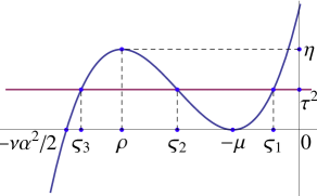
Figure 1. The graph of $f$ and solutions of $f(\varsigma)=\tau^{2}$.

Based on the derivative of $h_{\tau}$ given in (4), the behavior of $h_{\tau}$ is presented in Table 2 for $\tau^{2}>\eta$ and in Table 3 for $0<\tau^{2}\leq\eta$.

$\varsigma$	$-\infty$		$-\mu$		$\varsigma_{1}$		$+\infty$
$h_{\tau}^{\prime}(\varsigma)$		$+$	$|$	$+$	$0$	$-$	$0$
$h_{\tau}(\varsigma)$	$-\infty$	$\nearrow$	${}^{+\infty}|_{-\infty}$	$\nearrow$	$h_{\tau}(\varsigma_{1})$	$\searrow$	$-\infty$

Table 2. The behavior of $h$ for $\tau^{2}>\eta$.

$\varsigma$	$-\infty$		$\varsigma_{3}$		$\varsigma_{2}$		$-\mu$		$\varsigma_{1}$		$+\infty$
$h_{\tau}^{\prime}(\varsigma)$	$+$	$+$	$0$	$-$	$0$	$+$	$|$	$+$	$0$	$-$
$h_{\tau}(\varsigma)$	$-\infty$	$\nearrow$	$h_{\tau}(\varsigma_{3})$	$\searrow$	$h_{\tau}(\varsigma_{2})$	$\nearrow$	${}^{+\infty}|_{-\infty}$	$\nearrow$	$h_{\tau}(\varsigma_{1})$	$\searrow$	$-\infty$

Table 3. The behavior of $h$ for $0<\tau^{2}\leq\eta$.

Assume that $\tau\neq 0$. From the discussion above we have that the equation $f(\varsigma)=\tau^{2}$ has a unique solution $\overline{\varsigma}_{1}:=\varsigma_{1}$ on the interval $(-\mu,\infty)$. Since $\overline{\varsigma}_{1}>-\mu$, from Theorem 1 (v), (vi) we know that $(\overline{u}_{1},\overline{\varsigma}_{1})$ with $\overline{u}_{1}:=u_{\overline{\varsigma}_{1}}$ is a critical point of $\Xi_{\tau}$ and

$$\inf_{u\in\mathbb{R}}p_{\tau}(u)=p_{\tau}(\overline{u}_{1})=h_{\tau}(\overline{\varsigma}_{1})=\sup_{\varsigma>-\mu}h_{\tau}(\varsigma).$$

The fact that $h_{\tau}(\overline{\varsigma}_{1})>h_{\tau}(\varsigma)$ for $\varsigma\in(-\mu,\infty)\setminus\{\overline{\varsigma}_{1}\}$ is clear from Tables 2, 3. In order to complete (18) we have to prove that $\overline{u}_{1}$ is the only (strict) global minimum point for $p_{\tau}$, i.e., $p_{\tau}(u)>p_{\tau}(\overline{u}_{1})$ for $u\in\mathbb{R}\setminus\{\overline{u}_{1}\}.$

Assume that there exists $\overline{u}_{0}\in\mathbb{R}\setminus\{\overline{u}_{1}\}$ such that $p_{\tau}(\overline{u}_{0})=p_{\tau}(\overline{u}_{1})$. Hence $\overline{u}_{0}$ is a global minimum point of $p_{\tau}$. The polynomial $q(y)=p_{\tau}(y)-p_{\tau}(\overline{u}_{0})$ has degree 4, is non-negative, and admits the distinct roots $\overline{u}_{0},\overline{u}_{1}$. Hence $\overline{u}_{0},\overline{u}_{1}$ are double roots and so $q(y)=\tfrac{1}{8}\nu(y-\overline{u}_{0})^{2}(y-\overline{u}_{1})^{2}$ after one takes into account the leading coefficient of $p_{\tau}$. It follows that $p_{\tau}(y)=p_{\tau}(\overline{u}_{0})+\tfrac{1}{8}\nu(y-\overline{u}_{0})^{2}(y-\overline{u}_{1})^{2}$. In expanded form,

$$p_{\tau}(y)=\tfrac{1}{8}\nu y^{4}-\tfrac{1}{2}\nu\alpha y^{3}+(\tfrac{1}{2}\nu\alpha^{2}+\tfrac{1}{2}\mu)y^{2}-(\tau+\alpha\mu)y+p_{\tau}(0).$$

After we identify the coefficients of $y^{3},y^{2}$ and $y$ we find $\overline{u}_{0}+\overline{u}_{1}=2\alpha$, $\overline{u}_{0}\overline{u}_{1}=2\mu\nu^{-1}$, and $\tau=0$. Since by our running hypothesis $\tau\neq 0$, we obtain $p_{\tau}(u)>p_{\tau}(\overline{u}_{0})$ for all $\mathbb{R}\setminus\{\overline{u}_{1}\}.$

(a), (b) and the first part of (c) follow from the discussion above on $f$ and $\overline{\varsigma}_{1}.$

(c) Assume that $0<\tau^{2}<\eta$. The fact that $-\mu>\overline{\varsigma}_{2}>\rho>\overline{\varsigma}_{3}>-\tfrac{1}{2}\nu\alpha^{2}$ follows from Table 1. Also from the behavior of $h_{\tau}$ shown in Table 3 we have that

$$h_{\tau}(\overline{\varsigma}_{2})=\min_{\varsigma\in(\overline{\varsigma}_{3},-\mu)}h_{\tau}(\varsigma),\quad h_{\tau}(\overline{\varsigma}_{3})=\max_{\varsigma\in(-\infty,\overline{\varsigma}_{2})}h_{\tau}(\varsigma).$$

According to Theorem 1 $(\overline{u}_{i},\overline{\varsigma}_{i})$ is a critical point of $\Xi_{\tau}$, $p_{\tau}^{\prime}(\overline{u}_{i})=0$, $h_{\tau}(\overline{\varsigma}_{i})=p_{\tau}(\overline{u}_{i})$ and $p_{\tau}^{\prime\prime}(\overline{u}_{i})=3\left(\overline{\varsigma}_{i}-\rho\right)$ for $i\in\{2,3\}$. Because $\overline{\varsigma}_{2}>\rho>\overline{\varsigma}_{3}$, we have that $p_{\tau}^{\prime\prime}(\overline{u}_{2})>0$ and $p_{\tau}^{\prime\prime}(\overline{u}_{3})<0$, proving that $\overline{u}_{2}$ is a strict local minimum point of $p_{\tau}$ and $\overline{u}_{3}$ is a strict local maximum point of $p_{\tau}$.

(d) For $\tau=0$ we have

$$p_{0}(y)=\tfrac{1}{8}\nu\left(y^{2}-2\alpha y+2\nu^{-1}\mu\right)^{2}-\tfrac{1}{2}\nu^{-1}\mu^{2}=\tfrac{1}{8}\nu\left(y-\overline{u}_{1}\right)^{2}\left(y-\overline{u}_{2}\right)^{2}-\tfrac{1}{2}\nu^{-1}\mu^{2}.$$

Taking into account that $h_{0}(\varsigma)=-\frac{1}{2}\left[\alpha^{2}(\varsigma+\mu)+\nu^{-1}\varsigma^{2}\right]$ for $\varsigma\in\mathbb{R}$, relation (21) and the rest of the conclusion are straightforward. ∎

Corollary 3.

Assume that $2\mu<\nu\alpha^{2}$. With the notation of the preceding proposition, if $0<\tau^{2}<\eta$ then $p_{\tau}(\overline{u}_{3})>p_{\tau}(\overline{u}_{2})>p_{\tau}(\overline{u}_{1}).$

Proof.

Since $\overline{u}_{2}\neq\overline{u}_{1}$, from (18) we get $p_{\tau}(\overline{u}_{2})>p_{\tau}(\overline{u}_{1})$. Also, from (19), (20), and Table 3 $p_{\tau}(\overline{u}_{3})=h_{\tau}(\overline{\varsigma}_{3})>h_{\tau}(\overline{\varsigma}_{2})=p_{\tau}(\overline{u}_{2})$. ∎

3. Application to a nonconvex variational problem

Let us consider $\tau_{\theta},\alpha,\mu>0$, $0<a<b,$ $\sigma:[a,b]\rightarrow\mathbb{R}$ be defined by $\sigma(r):=b^{2}\tau_{\theta}r^{-2}$ and $\widehat{\mathcal{P}}:\mathcal{L}^{4}(a,b)\rightarrow\mathbb{R}$ be defined by

$$\widehat{\mathcal{P}}(v):=2\pi\int_{a}^{b}\left[\tfrac{1}{2}\mu r^{2}v^{2}+\tfrac{1}{2}\nu\left(\tfrac{1}{2}r^{2}v^{2}-\alpha rv\right)^{2}-\sigma v\right]rdr=2\pi\int_{a}^{b}rp_{-\beta}(rv)dr,$$ (22)

where $v\in\mathcal{L}^{4}(a,b)$, $\beta(r):=\alpha\mu-\sigma(r)$, $r\in[a,b]$, and $p_{-\beta}$ is defined via (1). In the previous formula and the subsequent ones we use $v,\sigma$, and $\beta$ instead of $v(r),\sigma(r)$, and $\beta(r)$ for the simplicity of notation.

Throughout this note we use the notation $\mathcal{L}^{p}:=\mathcal{L}^{p}(a,b)$, $p\geq 1$, and the convention $0/0:=0$, which agrees with the convention $0\cdot(\pm\infty):=0$ used in measure theory. With this convention in mind, consider

$$A_{1}:=\left\{\zeta\in\mathcal{L}^{2}\,\bigg{|}\,\frac{\beta^{2}}{\zeta+\mu}\in\mathcal{L}^{1}\right\};$$ (23)

and the function

$$\mathcal{P}^{d}:A_{1}\rightarrow\mathbb{R},\quad\mathcal{P}^{d}(\zeta):=-\pi\int_{a}^{b}\left(\frac{(\sigma+\alpha\zeta)^{2}}{\zeta+\mu}+\nu^{-1}\zeta^{2}\right)rdr.$$ (24)

Taking into account (26) below, $A_{1}$ is the biggest subset of $\mathcal{L}^{2}$ for which $\mathcal{P}^{d}$ is well defined, i.e, $\mathcal{P}^{d}(\zeta)\in\mathbb{R}$ iff $\zeta\in A_{1}$. Clearly,

$$A_{1}\subset A_{2}:=\left\{\zeta\in\mathcal{L}^{2}\mid\zeta(x)+\mu\neq 0\text{ for a.e. }x\in[a,b]\right\}.$$ (25)

Since

$$\frac{(\sigma+\alpha\zeta)^{2}}{\mu+\zeta}+\nu^{-1}\zeta^{2}=\frac{\beta^{2}}{\zeta+\mu}-2\alpha\beta+\alpha^{2}(\zeta+\mu)+\nu^{-1}\zeta^{2},$$ (26)

we have that,

$$\mathcal{P}^{d}(\zeta)=2\pi\int_{a}^{b}rh_{-\beta(r)}(r)dr,$$ (27)

where $h_{-\beta(r)}$ is given by (2) or (3).

Taking into account the expressions of $\widehat{\mathcal{P}}$ in (22) and $\mathcal{P}^{d}$ in (27) and after applying Proposition 2 for $\tau=-\beta(r)$ we get the following result.

Proposition 4.

Assume that $2\mu<\nu\alpha^{2}$.

(a) If $\beta^{2}>\eta$ on $[a,b]$, (that is, $\beta^{2}(r)>\eta$ for every $r\in[a,b]$) then equation (9) corresponding to $\tau=-\beta$ has a unique solution $\overline{\zeta}\in C[a,b]\cap A_{1}$ with $\overline{\zeta}>-\mu$ on $[a,b]$, and for $\overline{v}:=r^{-1}\left(\alpha-\beta/(\overline{\zeta}+\mu)\right)$ one has

$$\widehat{\mathcal{P}}\mathcal{(}\overline{v})=\min_{v\in\mathcal{L}^{4}}\widehat{\mathcal{P}}(v)=\max_{\zeta\in A_{1},\zeta>-\mu}\mathcal{P}^{d}(\zeta)=\mathcal{P}^{d}(\overline{\zeta}).$$ (28)

(b) If $0<\beta^{2}<\eta$ on $[a,b]$ then equation (9) corresponding to $\tau=-\beta$ has three solutions $\overline{\zeta}_{1},\overline{\zeta}_{2},\overline{\zeta}_{3}\in C[a,b]\cap A_{1}$ with $\overline{\zeta}_{1}>-\mu>\overline{\zeta}_{2}>\rho>\overline{\zeta}_{3}>-\tfrac{1}{2}\nu\alpha^{2}$ on $[a,b]$. Moreover, for $\overline{v}_{i}:=r^{-1}\left(\alpha-\beta/(\overline{\zeta}_{i}+\mu)\right)$ $(i\in\{1,2,3\})$, one has

$$\widehat{\mathcal{P}}\mathcal{(}\overline{v}_{1})=\min_{v\in\mathcal{L}^{4}}\widehat{\mathcal{P}}(v)=\max_{\zeta\in A_{1},\zeta>-\mu}\mathcal{P}^{d}(\zeta)=\mathcal{P}^{d}(\overline{\zeta}_{1}),$$ (29)

$$\widehat{\mathcal{P}}\mathcal{(}\overline{v}_{2})=\min_{\zeta\in A_{1},\overline{\zeta}_{3}<\zeta<-\mu}\mathcal{P}^{d}(\zeta)=\mathcal{P}^{d}(\overline{\zeta}_{2}),$$ (30)

$$\widehat{\mathcal{P}}\mathcal{(}\overline{v}_{3})=\max_{\zeta\in A_{1},\zeta<\overline{\zeta}_{2}}\mathcal{P}^{d}(\zeta)=\mathcal{P}^{d}(\overline{\zeta}_{3}).$$ (31)

Proof.

The existence and continuity of the solutions $\overline{\zeta}$ in case (a) and $\overline{\zeta}_{1}$, $\overline{\zeta}_{2},$ $\overline{\zeta}_{3}$ in case (b) follow from the behavior of $f$ presented in Table 1 and the fact that $\beta\in C^{\infty}[a,b]$. More precisely, the critical point of $f$ are $-\mu$ and $\rho$ with $f(-\mu)=0$, $f(\rho)=\eta$ (see Table 1) so the inverses of $f$ restricted to each of the intervals $(-\tfrac{1}{2}\nu\alpha^{2},\rho)$, $(\rho,-\mu)$, $(-\mu,\infty)$ exist and are smooth. Since for $\beta^{2}>0$ the solution $\varsigma(r)$ of the equation $f(\varsigma)=\beta^{2}(r)$ is different from $-\mu$, we have that $\overline{\zeta},\overline{\zeta}_{1},\overline{\zeta}_{2},\overline{\zeta}_{3}\in A_{1}$ and $\overline{v},\overline{v}_{1},\overline{v}_{2},\overline{v}_{3}$ are continuous and implicitly belong to $\mathcal{L}^{4}.$

(a) For every $v\in\mathcal{L}^{4}$ and $\zeta\in A_{1}$ with $\zeta>-\mu$ on $[a,b]$, apply Proposition 2(a) for a fixed $r\in[a,b]$, $u:=rv(r)$, and $\varsigma:=\zeta(r)$ to obtain

$$p_{-\beta(r)}(rv(r))\geq p_{-\beta(r)}(r\overline{v}(r))=h_{-\beta(r)}(\overline{\zeta}(r))\geq h_{-\beta(r)}(\zeta(r)).$$

Multiplying by $2\pi r>0$ and integrating on $[a,b]$ provide

$$\widehat{\mathcal{P}}\mathcal{(}v)\geq\widehat{\mathcal{P}}\mathcal{(}\overline{v})=\mathcal{P}^{d}(\overline{\zeta})\geq\mathcal{P}^{d}(\zeta)$$

for all $v\in\mathcal{L}^{4}$ and $\zeta\in A_{1}$ with $\zeta>-\mu$. The conclusion follows. The proof for (b) follows similarly from Proposition 2(c).∎

4. Some comments on [3, Th. 4]

On [3, p. 502] one says:

$\bullet$ “we consider the kinetically admissible space to be defined by

$\mathcal{X}_{a}=\{g(r)\in\mathcal{C}[a,b]\mid g^{\prime}\in\mathcal{L}^{p}[a,b],~{}g(a)=0\},\quad(19)$

where $\mathcal{L}^{p}$ is the space of Lebesgue integrable functions for some $p\in[1,\infty)$.”

followed by:

$\bullet$ “Then the considered problem can be formulated as the following minimization problem for the determination of the deformation function $g$:

$\min\limits_{g\in\mathcal{X}_{a}}\left\{\mathcal{P}(g)=2\pi{\displaystyle\int_{a}^{b}}\hat{W}(rg^{\prime}(r))rdr-2\pi b^{2}\tau_{\theta}g(b)\right\}$.    (20)”

Later on (see [3, p. 506]) one says:

$\bullet$ “In this section the strain energy is assumed to be the nonconvex function of the shear strain $\gamma$ given by

$\hat{W}(\gamma)=\tfrac{1}{2}\mu\gamma^{2}+\tfrac{1}{2}\nu\left(\tfrac{1}{2}\gamma^{2}-\alpha\gamma\right)^{2}$,    (39)

where $\mu>0$, $\nu>0$ and $\alpha\in\mathbb{R}$ are material constants.”

On the next page one continues with

$\bullet$ “… there is no loss of generality in restricting attention to $\alpha>0$, which we do here.”,

$\bullet$ “The parameters $\alpha,\mu,\nu$ are then such that

$2\mu<\nu\alpha^{2}<8\mu$,    (40)

and for the most part we restrict attention to this range of values.”,

$\bullet$ “In this section, therefore, we restrict attention to the more interesting case for which $\tau_{\theta}>0$, and hence $\gamma>0$.

For this situation we define a two-component canonical strain measure $\mathbf{\xi}$ by

$\mathbf{\xi}=(\varepsilon,\xi)=\Lambda(g)=\left(\tfrac{1}{2}(rg^{\prime})^{2},\tfrac{1}{2}(rg^{\prime})^{2}-\alpha(rg^{\prime})\right)\in\mathbb{R}^{2},$

and the canonical energy $U(\mathbf{\xi})=\mu\varepsilon+\tfrac{1}{2}\nu\xi^{2}$ is then a convex (quadratic) function, which is well defined on the domain

$\mathcal{E}=\{(\varepsilon,\xi)\in\mathcal{L}^{1}\times\mathcal{L}^{2}\mid\varepsilon(r)\geq 0,~{}\xi(r)\geq-\tfrac{1}{2}\alpha^{2},\ \forall r\in[a,b]\}$.

The canonical dual ‘stress’ vector

$\mathbf{\zeta}=(\varsigma,\zeta)=U_{\mathbf{\xi}}(\mathbf{\xi})=(\mu,\nu\xi)\in\mathbb{R}^{2},$

where $U_{\mathbf{\xi}}(\mathbf{\xi})=\partial U/\partial\xi$, is well defined on the dual space

$\mathcal{S}=\{(\varsigma,\zeta)\in\mathcal{L}^{\infty}\times\mathcal{L}^{2}\mid\varsigma(r)=\mu,~{}\zeta(r)\geq-\tfrac{1}{2}\nu\alpha^{2},forallr\in[a,b]\}$.”

and

$\bullet$ “… we obtain the total complementary energy $X(g,\zeta)$ for this nonconvex problem in the form

$X(g,\zeta)=...=2\pi\int_{a}^{b}\left[\tfrac{1}{2}(rg^{\prime})^{2}(\zeta+\mu)-\alpha rg^{\prime}\zeta-\tfrac{1}{2}\nu^{-1}\zeta^{2}\right]rdr-2\pi b^{2}\tau_{\theta}g(b)$.   (41)”

Page 509 of [3] begins with:

$\bullet$ “For a given $\mathbf{\zeta}\in\mathcal{S}$, the criticality condition $\delta_{g}X(g,\zeta)=0$ leads to the equation

$\left((\zeta+\mu)r^{3}g^{\prime}-r^{2}\alpha\zeta\right)^{\prime}=0,\quad r\in(a,b),$

and the boundary condition

$(\zeta+\mu)r^{3}g^{\prime}-r^{2}\alpha\zeta=b^{2}\tau_{\theta}\quad$on$\quad r=b$.”

followed by

$\bullet$ “Therefore, by substituting $\gamma=rg^{\prime}=(\sigma+\alpha\zeta)/(\zeta+\mu)$ into $X$, the pure complementary energy $\mathcal{P}^{d}$ can be obtained by the canonical dual transformation

$\mathcal{P}^{d}(\zeta)=\left\{X(g,\zeta)\mid\delta_{g}X(g,\zeta)=0\right\}=-\pi{\displaystyle\int_{a}^{b}\left(\frac{(\sigma+\alpha\zeta)^{2}}{\zeta+\mu}+\nu^{-1}\zeta^{2}\right)}rdr$,    (42)

which is well defined on the dual feasible space

$\mathcal{S}_{a}=\left\{\zeta\in\mathcal{L}^{2}\mid\zeta(r)+\mu\neq 0,\right\}.$

The criticality condition $\delta\mathcal{P}^{d}(\zeta)=0$ leads to the dual algebraic equation

$\left(2\nu^{-1}\zeta+\alpha^{2}\right)(\mu+\zeta)^{2}=(\sigma-\mu\alpha)^{2}$.    (43)”.

On page 510 of [3] one can find:

$\bullet$ “… for simplicity of expression, we have introduced the notations $\beta=\mu\alpha-\sigma$ and

$\eta=(\nu\alpha^{2}-2\mu)^{3}/27\nu$.    (48)”

Note that $\mathcal{P}^{d}(\zeta)$ is exactly as in (24).

Before quoting the result we have in view let us shortly discuss the quoted text above.

Note that $\sigma(r)=b^{2}\tau_{\theta}/r^{2}$ (as taken at the beginning of our Section 3), is mentioned on page 509 of [3] (see also [3, page 505]); probably one takes $0<a<b<\infty,$ assumptions that we accept here. Hence the set $B_{0}:=\{s\in[a,b]\mid\beta(s)=0\}$ has at most one element.

Probably, by “well defined on … $\mathcal{S}_{a}$” above one means that $\mathcal{P}^{d}(\zeta)\in\mathbb{R}$ for every $\zeta\in\mathcal{S}_{a},$ that is, $\mathcal{S}_{a}\subset A_{1}$ [see (23)]. But this inclusion is false as we will see from the next result. However $\mathcal{S}_{a}\subset A_{2}$.

Lemma 5.

Under the current notations and assumptions $\mathcal{S}_{a}\not\subset A_{1}$ and $\mathcal{P}^{d}$ is not well defined on $\mathcal{S}_{a}$.

Proof.

Recall that $\beta(r)=\alpha\mu-b^{2}\tau_{\theta}/r^{2}$ and note that $B_{0}=\{s\in[a,b]\mid\beta(s)=0\}\subset\{\sqrt{b^{2}\tau_{\theta}/(\alpha\mu)}\}$ so there exist $(c,d)\subset(a,b)$ and $\gamma>0$ such that $\beta^{2}(x)\geq\gamma$ for every $x\in[c,d]$. Let $\zeta(r)=-\mu+r-c$ for $r\in(c,d)$, $\zeta(r)=1-\mu$ for $r\in[a,b]\setminus(c,d)$. Then $\zeta\in\mathcal{L}^{2}$ and $\zeta>-\mu>-\tfrac{1}{2}\nu\alpha^{2}$ on $[a,b]$, i.e., $\zeta\in\mathcal{S}_{a}$. Also $\frac{\beta^{2}}{\zeta+\mu}\geq\frac{\gamma}{\zeta+\mu}>0$ on $[c,d]$ and $\int_{a}^{b}\frac{\beta^{2}(r)}{\zeta(r)+\mu}dr\geq\gamma\int_{c}^{d}\frac{dr}{r-c}=+\infty$, that is $\zeta\not\in A_{1}$. ∎

Let us denote the algebraic interior (or core) of a set by “$\operatorname*{core}$”.

Lemma 6.

Under the current notations and assumptions $\operatorname*{core}A_{2}$ is empty. In particular, $\operatorname*{core}A_{1}=\operatorname*{core}\mathcal{S}_{a}=\emptyset$.

Proof.

Indeed, because $\sigma$ is continuous, there exist $\overline{\delta}>0$ and $a\leq a^{\prime}<b^{\prime}\leq b$ such that $\left|\beta\left(r\right)\right|\geq\overline{\delta}>0$ for every $r\in I=(a^{\prime},b^{\prime})$. Take $\overline{\zeta}\in A_{2}$ and define $u$ by $u(r)=n\big{[}a^{\prime}+\frac{b^{\prime}-a^{\prime}}{n}-r-\overline{\zeta}(r)-\mu\big{]}$ for $r\in[a^{\prime}+\frac{b^{\prime}-a^{\prime}}{n+1},a^{\prime}+\frac{b^{\prime}-a^{\prime}}{n})$ with $n\geq 1$, and $u(r)=0$ for $r\in[a,b]\setminus I$. Then for every $\delta>0$ there exists $t=\frac{1}{n}\in(0,\delta)$ such that $\overline{\zeta}+tu\notin A_{2}$. (Note that for $\overline{\zeta}\in A_{1}$ and for $u$ constructed as above we have that for every $\delta>0$ there exists $t\in(0,\delta)$ such that $\overline{\zeta}+tu\notin A_{1}$). ∎

To our knowledge, one can speak about Gâteaux differentiability of a function $f:E\subset X\rightarrow Y$, with $X,Y$ topological vector spaces, at $\overline{x}\in E$ only if $\overline{x}$ is in the core of $E$. As we have seen above, $\mathcal{P}^{d}(\zeta)\in\mathbb{R}$ only for $\zeta\in A_{1}$ and $\operatorname*{core}A_{1}=\emptyset.$ These considerations naturally lead to the following question:

In what sense is the critical point notion associated to $\mathcal{P}^{d}$ understood so that when using this notion one gets [3, (43)], other than just formal computation?

Taking into account the comment (see [3, page 509])

$\bullet$ “We emphasize that the integrand of $\mathcal{P}^{d}(\zeta)$ has a singularity at $\zeta=-\mu$, which is excluded in the definition of $\mathcal{S}_{a}$, and does not in general correspond to a critical point of $\mathcal{P}^{d}(\zeta)$”,

we wish to point out that there is an important difference between the condition $\zeta\neq-\mu$ and $\zeta(r)\neq-\mu$ a.e. on $[a,b]$ since it is known that $\zeta\neq-\mu$ means that $\zeta(x)\neq-\mu$ on a set of positive measure. Alternatively, $\mathcal{L}^{2}\setminus\{-\mu\}$ is a (nonempty) open set, while, as seen above, the set $A_{2}:=\left\{\zeta\in\mathcal{L}^{2}\mid\zeta(r)+\mu\neq 0\text{ for a.e. }r\in[a,b]\right\}$ has empty core (in particular has empty interior).

From the quoted text it seems that $\zeta$ is taken from $\mathcal{L}^{2}$, but it is not very clear from where $g$ is taken; apparently $g\in\mathcal{X}_{a}$, that is, $g\in\mathcal{C}[a,b]$ is such that $g^{\prime}\in\mathcal{L}^{p}$ and $g(a)=0$ for some fixed $p\in[1,\infty)$. But, to have $(\varepsilon,\xi)\in\mathcal{L}^{1}\times\mathcal{L}^{2}$ where $\varepsilon(r)=\tfrac{1}{2}(rg^{\prime}(r))^{2}$ and $\xi(r)=\tfrac{1}{2}(rg^{\prime}(r))^{2}-\alpha rg^{\prime}(r)$ one needs $p\geq 4$. Moreover, the statement $\left(\tfrac{1}{2}(rg^{\prime})^{2},\tfrac{1}{2}(rg^{\prime})^{2}-\alpha(rg^{\prime})\right)\in\mathbb{R}^{2}$ is quite strange because $g^{\prime}$ is a function (or even an equivalent class).

In the sequel we take $p=4$. Then $g$ in $\mathcal{X}_{a}$ has to be an absolutely continuous function on $[a,b]$ with $g(a)=0$ and $g^{\prime}\in\mathcal{L}^{4}[a,b]$. In fact

$$g\in\mathcal{X}_{a}\Longleftrightarrow\exists v\in\mathcal{L}^{4},\ {\rm for\ all}\ r\in[a,b]:g(r)=\int_{a}^{r}v(t)dt.$$

So, the problem $\min_{g\in\mathcal{X}_{a}}\mathcal{P}(g)$ above becomes the problem $\min_{v\in\mathcal{L}^{4}}\widehat{\mathcal{P}}(v)$ with $\widehat{\mathcal{P}}(v)$ defined in (22).

Next, using the above considerations we discuss the following result of [3]; we also quote its proof for easy reference.

“Theorem 4 (Extremality Criteria). For a given shear stress $\tau_{\theta}>0$ such that $\sigma=b^{2}\tau_{\theta}/r^{2}$, if $(\sigma-\alpha\mu)^{2}>\eta>0$ the dual algebraic equation (43) has a unique real root $\overline{\zeta}(r)>-\mu$, which is a global maximizer of $\mathcal{P}^{d}$ over $\mathcal{S}_{a}$, and the corresponding solution $\overline{g}$ is a global minimizer of $\mathcal{P}(g)$ over $\mathcal{X}_{a}$, i.e.

$\mathcal{P(}\overline{g})=\min\limits_{g\in\mathcal{X}_{a}}\mathcal{P}(g)=\max\limits_{\zeta\in\mathcal{S}_{a}}\mathcal{P}^{d}(\zeta)=\mathcal{P}^{d}(\overline{\zeta})$.    (51)

If $(\sigma-\alpha\mu)^{2}<\eta$ and $\sigma\neq\alpha\mu$ then equation (43) has three real roots ordered as (49). The corresponding solution $\overline{g}_{1}$ is a global minimizer of $\mathcal{P}(g)$ and $\overline{\zeta}_{1}$ is a global maximizer of $\mathcal{P}^{d}(\zeta)$ over the domain $\zeta>-\mu$, i.e.

$\mathcal{P(}\overline{g})=\min\limits_{g\in\mathcal{X}_{a}}\mathcal{P}(g)=\max\limits_{\zeta>-\mu}\mathcal{P}^{d}(\zeta)=\mathcal{P}^{d}(\overline{\zeta}_{1})$.    (52)

For $\overline{\zeta}_{2}$, the corresponding solution $\overline{g}_{2}$ is a local minimizer of $\mathcal{P}(g)$, while for $\overline{\zeta}_{3}$ the associated $\overline{g}_{3}$ is a local maximizer, so that

$\mathcal{P(}\overline{g}_{2})=\min\limits_{g\in\mathcal{X}_{2}}\mathcal{P}(g)=\min\limits_{\overline{\zeta}_{3}<\zeta<-\mu}\mathcal{P}^{d}(\zeta)=\mathcal{P}^{d}(\overline{\zeta}_{2})$,    (53)

and

$\mathcal{P(}\overline{g}_{3})=\max\limits_{g\in\mathcal{X}_{3}}\mathcal{P}(g)=\max\limits_{-\tfrac{1}{2}\nu\alpha^{2}<\zeta<\overline{\zeta}_{2}}\mathcal{P}^{d}(\zeta)=\mathcal{P}^{d}(\overline{\zeta}_{3})$,    (54)

where $\mathcal{X}_{i}$ is a neighborhood of $\overline{g}_{i}$ for $i=2,3$.

In the transitional cases for which $\sigma-\alpha\mu=\pm\sqrt{\eta}$, the two roots $\overline{\zeta}_{2}$ and $\overline{\zeta}_{3}$ coincide and the local extrema described by (53) and (54) merge into a horizontal point of inflection. In the case $\sigma=\alpha\mu$ the two roots $\overline{\zeta}_{1}$ and $\overline{\zeta}_{2}$ coincide at $-\mu$ and this is the transitional point at which the two local minima are equal and the solution becomes nonsmooth.

Proof. The proof of this theorem follows from the triality theory developed in [5, 8]. $\quad\square$”

The references [5, 8] above are our references [1] and [2], respectively.

Before discussing the above result let us clarify the meaning for $\overline{\zeta}_{i}$ and $\overline{g}_{i}$ (as well as $\overline{\zeta}$ and $\overline{g}$) appearing in the above statement. In fact these functions are defined in the statement of [3, Th. 2]:

“Theorem 2 (Closed-form Solutions). For a given shear stress $\tau_{\theta}>0$ such that $\sigma=b^{2}\tau_{\theta}/r^{2}$, the dual algebraic equation (43) has at most three real roots $\overline{\zeta}_{i}(r)$, $i=1,2,3$, ordered as

$\overline{\zeta}_{1}(r)\geq-\mu\geq\overline{\zeta}_{2}(r)\geq\overline{\zeta}_{3}(r)\geq-\tfrac{1}{2}\nu\alpha^{2}$.    (49)

For each of these roots, the function defined by

$\overline{g}_{i}(r)=\int_{a}^{r}\frac{b^{2}\tau_{\theta}/s^{2}+\alpha\overline{\zeta}_{i}(s)}{s\left(\overline{\zeta}_{i}(s)+\mu\right)}ds\quad$ (50)

is a solution of the boundary value problem (BVP), and

$\mathcal{P}(\overline{g}_{i})=\mathcal{P}^{d}(\overline{\zeta}_{i}),~{}~{}i=1,2,3$.”

With our reformulation of the problem [3, (20)] in place, in the statements of [3, Th. 2, Th. 3] one must replace $\mathcal{X}_{a}$ by $\mathcal{L}^{4}$, $\overline{g}_{i}$ by $\overline{v}_{i}:=\frac{\sigma+\alpha\overline{\zeta}_{i}}{r(\overline{\zeta}_{i}+\mu)},$ $\overline{g}$ by $\overline{v}:=\frac{\sigma+\alpha\overline{\zeta}}{r(\overline{\zeta}+\mu)}$ and $\mathcal{P}$ by $\widehat{\mathcal{P}}$, $\mathcal{X}_{j}$ being now a neighborhood of $\overline{v}_{j}$, for $j=2,3$. This is possible since the operator $v\in\mathcal{L}^{4}\rightarrow u=\int_{a}^{r}v\in\mathcal{X}_{a}$ and its inverse $\mathcal{X}_{a}\ni u\rightarrow v=u_{x}\in\mathcal{L}^{4}$ are linear continuous under the $W^{1,4}$ topology on $\mathcal{X}_{a}$; whence $g\in\mathcal{X}_{a}$ is a local extrema for $\mathcal{P}$ iff the corresponding $v\in\mathcal{L}^{4}$ is a local extrema for $\widehat{\mathcal{P}}$.

Hence $\overline{\zeta}$, $\overline{\zeta}_{i}$ and $\overline{v},$ $\overline{v}_{i}$ are exactly as in our Proposition 4. We observe that there are differences between the conclusions of Proposition 4 and [3, Th. 4], the conclusions in [3, Th. 4] being stronger. In the discussion below we show that it is not possible to obtain stronger conclusions than those of Proposition 4.

Discussion of [3, (51)]. The sole difference between [3, (51)] and (28) is that one has $\max_{\zeta\in\mathcal{S}_{a}}\mathcal{P}^{d}(\zeta)$ instead of $\max_{\zeta\in A_{1},\zeta>-\mu}\mathcal{P}^{d}(\zeta)$. As seen Section 3, $\mathcal{P}^{d}(\zeta)\in\mathbb{R}$ only for $\zeta\in A_{1}$, so considering $\sup_{\zeta\in\mathcal{S}_{a}}\mathcal{P}^{d}(\zeta)$ makes no sense. One can ask if [3, (51)] holds when one replaces $\max_{\zeta\in\mathcal{S}_{a}}\mathcal{P}^{d}(\zeta)$ by $\max_{\zeta\in A_{1}^{0}}\mathcal{P}^{d}(\zeta)$, where

$$A_{1}^{0}:=\{\zeta\in A_{1}\mid\zeta\geq-\tfrac{1}{2}\nu\alpha^{2}\}.$$

That is not true. Indeed, consider $\zeta_{n}(r)=-\mu-\gamma(r-a)$ for $r\in[a+(b-a)/n,b]$ and $\zeta_{n}(r)=-\mu-\gamma(b-a)/n$ for $r\in[a,a+(b-a)/n)$, where $0<\gamma<\left(\tfrac{1}{2}\nu\alpha^{2}-\mu\right)/(b-a)$. Clearly $-\mu-\gamma(b-a)/n\geq\zeta_{n}\geq-\mu-\gamma(b-a)>-\tfrac{1}{2}\nu\alpha^{2}$ on $[a,b]$, and so $\zeta_{n}\in A_{1}^{0}$. Moreover

$$-\int_{a}^{b}\frac{\beta^{2}}{\zeta_{n}+\mu}dr\geq\int_{a+(b-a)/n}^{b}\frac{\beta^{2}(r)}{\gamma(r-a)}dr\geq\frac{\eta}{\gamma}\ln n\rightarrow\infty,$$

which proves that $\sup_{\zeta\in A_{1}^{0}}\mathcal{P}^{d}(\zeta)=+\infty$ (see (24)).

Discussion of [3, (52)]. A similar discussion as above shows that $\max_{\zeta>-\mu}\mathcal{P}^{d}(\zeta)$ in [3, (52)] does not make sense. The correct equality has been established in (29).

Discussion of [3, (53)]. Assume that $0<\beta^{2}<\eta$ on $[a,b]$. It is easy to show that $\{\zeta\in\mathcal{L}^{2}\mid\rho<\zeta<-\mu\}\not\subset A_{1}$, which proves that $\{\zeta\in\mathcal{L}^{2}\mid\overline{\zeta}_{3}<\zeta<-\mu\}\not\subset A_{1}$; take for example $\zeta(r)=-\mu+\frac{\rho+\mu}{\eta}(r-a)\beta^{2}(r)$, $r\in(a,b)$. This shows that $\min_{\overline{\zeta}_{3}<\zeta<-\mu}\mathcal{P}^{d}(\zeta)$ in [3, (53)] does not make sense. Therefore one has to replace the set $\{\zeta\in\mathcal{L}^{2}\mid\overline{\zeta}_{3}<\zeta<-\mu\}$ by $\{\zeta\in A_{1}\mid\overline{\zeta}_{3}<\zeta<-\mu\}$, that is, as in (30).

The problem that occurs now is whether $\overline{v}_{2}$ is a local minimum point of $\widehat{\mathcal{P}}$. The answer for this problem is negative. Indeed, consider $\varepsilon\in(0,b-a)$ and take $v_{\varepsilon}(r):=\overline{v}_{1}(r)$ for $r\in[a,a+\varepsilon]$, $v_{\varepsilon}(r):=\overline{v}_{2}(r)$ for $r\in(a+\varepsilon,b]$. From Corollary 3 we have that $p_{-\beta(r)}(rv_{\varepsilon}(r))<p_{-\beta(r)}(r\overline{v}_{2}(r))$ for every $r\in[a,a+\varepsilon]$, and so

$$\widehat{\mathcal{P}}(\overline{v}_{2})-\widehat{\mathcal{P}}(v_{\varepsilon})=2\pi\int_{a}^{a+\varepsilon}r\left[p_{-\beta(r)}(r\overline{v}_{2}(r))-p_{-\beta(r)}(rv_{\varepsilon}(r))\right]dr>0.$$

Since $\left\|v_{\varepsilon}-\overline{v}_{2}\right\|=\big{(}\int_{a}^{a+\varepsilon}\left|\overline{v}_{2}-\overline{v}_{1}\right|^{4}\big{)}^{1/4}\leq\varepsilon^{1/4}\left\|\overline{v}_{2}-\overline{v}_{1}\right\|,$ it is clear that $\overline{v}_{2}$ is not a local minimum point of $\widehat{\mathcal{P}}.$

Discussion of [3, (54)]. Clearly, $\{\zeta\in\mathcal{L}^{2}\mid-\tfrac{1}{2}\nu\alpha^{2}<\zeta<\overline{\zeta}_{2}\}\subset A_{1};$ hence the last equality in [3, (54)] holds due to Proposition 4 (b) and relation (31). As above, now the problem is whether $\overline{v}_{3}$ is a local maximum point of $\widehat{\mathcal{P}}$. The answer is negative. Indeed, as seen in Proposition 4, $\overline{\zeta}_{3}\in C[a,b]$, $\overline{\zeta}_{3}<\rho<-\mu$ on $[a,b]$ so $\overline{v}_{3}\in C[a,b]$. It follows that the mapping $q:[a,b]\rightarrow\mathbb{R}$ defined by $q(r):=p_{-\beta(r)}(r\overline{v}_{3}(r))$ is continuous, and so $M:=\max_{[a,b]}q\in\mathbb{R}$. Set $m:=\max_{[a,b]}\left|\beta\right|>0$. It follows that

$$p_{-\beta(r)}(y) =\tfrac{1}{2}\mu y^{2}+\tfrac{1}{2}\nu\left(\tfrac{1}{2}y^{2}-\alpha y\right)^{2}-\alpha\mu y+\beta(r)y$$

$$\geq\tfrac{1}{2}\mu y^{2}+\tfrac{1}{2}\nu\left(\tfrac{1}{2}y^{2}-\alpha y\right)^{2}-\alpha\mu y-my=p_{m}(y)$$

for all $r\in[a,b]$ and $y\geq 0$. Since $\lim_{y\rightarrow\infty}p_{m}(y)=\infty$, there exists $y_{0}>0$ such that $p_{m}(y)>M$ for all $y\geq y_{0}$. Let us take $\overline{y}>0$ such that $a\overline{y}\geq y_{0}$ (and so $r\overline{y}\geq y_{0}$ for every $r\in[a,b]$). Consider $\varepsilon\in(0,b-a)$ and $v_{\varepsilon}(r):=\overline{y}$ for $r\in[a,a+\varepsilon]$, $v_{\varepsilon}(r):=\overline{v}_{3}(r)$ for $r\in(a+\varepsilon,b]$. We have that $p_{-\beta(r)}(r\overline{v}_{3}(r))\leq M<p_{m}(r\overline{y})\leq p_{-\beta(r)}(r\overline{y})$ for every $r\in[a,a+\varepsilon]$, and so

$$\widehat{\mathcal{P}}(\overline{v}_{3})-\widehat{\mathcal{P}}(v_{\varepsilon})=2\pi\int_{a}^{a+\varepsilon}r\left[p_{-\beta(r)}(r\overline{v}_{3}(r))-p_{-\beta(r)}(r\overline{y})\right]dr<0.$$

Since $\left\|v_{\varepsilon}-\overline{v}_{3}\right\|=\big{(}\int_{a}^{a+\varepsilon}\left|\overline{v}_{3}-\overline{y}\right|^{4}\big{)}^{1/4}\leq\varepsilon^{1/4}\left\|\overline{v}_{3}-\overline{y}\right\|$, this proves that $\overline{v}_{3}$ is not a local maximum of $\widehat{\mathcal{P}}.$

5. Conclusions

• The function $\mathcal{P}^{d}$ is not well defined on the set $\mathcal{S}_{a}.$ The biggest set on which $\mathcal{P}^{d}$ is well defined is $A_{1}$ whose core is empty; hence it is not possible to speak about critical points using the Gâteaux differential.

• Since $\mathcal{P}^{d}$ is not well defined on the sets $\mathcal{S}_{a},$ $\{\zeta\in\mathcal{L}^{2}\mid\zeta>-\mu\}$ and $\{\zeta\in\mathcal{L}^{2}\mid\overline{\zeta}_{3}<\zeta<-\mu\}$ the quantities $\max_{\zeta\in\mathcal{S}_{a}}\mathcal{P}^{d}(\zeta),$ $\max_{\zeta>-\mu}\mathcal{P}^{d}(\zeta)$ and $\min_{\overline{\zeta}_{3}<\zeta<-\mu}\mathcal{P}^{d}(\zeta)$ in [3, Th. 4] make no sense.

• The element $\overline{g}_{2}$ is not a local minimizer of $\mathcal{P}$ and $\overline{g}_{3}$ is not a local maximizer of $\mathcal{P}.$

• As seen above, one says that the proof of [3, Th. 4] “follows from the triality theory”, without mentioning a precise result. In fact, as seen in Section 3, the proof of the correct variant of [3, Th. 4], that is, Proposition 4, follows from an elementary result, while [3, Th. 4] is obtained by a simple extrapolation of Proposition 2.

References

- [1] D. Y. Gao, Duality, triality and complementary extremum principles in non-convex parametric variational problems with applications, IMA J. Appl. Math. 61 (1998) 199–235.
- [2] D. Y. Gao, Duality Principles in Nonconvex Systems: Theory, Methods and Applications (Kluwer, Dordrecht 2000).
- [3] D. Y. Gao, R. W. Ogden, Closed-form solutions, extremality and nonsmoothness criteria in a large deformation elasticity problem, Z. angew. Math. Phys. 59 (2008), 498–517.
- [4] D. Y. Gao, G. Strang, Geometric nonlinearity: Potential energy, complementary energy, and the gap function, Quart. Appl. Math. 47 (1989), 487–504.