CERN-PH-TH/2012-033

High-energy asymptotic behavior of the

Bourrely-Soffer-Wu model for elastic

scattering

Claude Bourrely Aix-Marseille Université,

Département de Physique, Faculté des Sciences de Luminy,

13288 Marseille, Cedex 09, France

John M. Myers School of Engineering and Applied Sciences

Harvard University, Cambridge, MA 02138, USA

Jacques Soffer Physics Department, Temple University

Barton Hall, 1900 N, 13th Street

Philadelphia, PA 19122-6082, USA
Tai Tsun Wu Harvard University, Cambridge, MA 02138, USA and

Theoretical Physics Division, CERN, 1211 Geneva 23, Switzerland

Abstract

Some time ago, an accurate phenomenological approach, the BSW model, was developed for proton-proton and antiproton-proton elastic scattering cross sections at center-of-mass energies above 10 GeV. This model has been used to give successful theoretical predictions for these processes, at successive collider energies.

The BSW model involves a combination of integrals that, while computable numerically at fairly high energies, require some mathematical analysis to reveal the high-energy asymptotic behavior. In this paper we present a high-energy asymptotic representation of the scattering amplitude at moderate momentum transfer, for the leading order in an expansion parameter closely related to the logarithm of the center-of-mass energy.

The fact that the expansion parameter goes as the logarithm of the energy means that the asymptotic behavior is accurate only for energies greatly beyond any foreseeable experiment. However, we compare the asymptotic representation against the numerically calculated model for energies in a less extreme region of energy. The asymptotic representation is given by a simple formula which, in particular, exhibits the oscillations of the differential cross section with momentum transfer. We also compare the BSW asymptotic behavior with the Singh-Roy unitarity upper bound for the diffraction peak.

Key words : elastic scattering, total cross section, differential cross section

PACS numbers : 11.80.Fv, 13.85.Dz, 13.85.Lg, 25.40.Cm

1 Introduction

Forty years ago, it was found theoretically, on the basis of quantum field theory, that, contrary to the general belief at the time, the total cross sections for hadronic scattering increases monotonically without limit at high energies [1]. In order to make predictions that could be verified by later experiments, it was essential to develop an accurate phenomenology with the following characteristics:
(i) - it agrees with the above theoretical asymptotic result at high energies,
(ii) - it describes the experimental data at energies available at that time.

Such a phenomenological model, termed the BSW model, was formulated by three of us [2, 3, 4].

Our model belongs to a class of models attempting to describe with different approaches in the eikonal formalism the high energy behavior of p p elastic scattering, let us mention a non exhaustive list [5]-[9].

In this paper, after reviewing the BSW phenomenological model for the elastic scattering amplitude, we present our predictions for LHC energies and derive an asymptotic representation for the scattering amplitude for extremely high center-of-mass energies.

In section 2 we recall the basic features of the impact picture approach (BSW), with its phenomenological parameters, and the expression of the scattering amplitude used in the next sections. In section 3 we present our predictions for the LHC energies at $\sqrt{s}=7,~{}14\mbox{GeV}$ and make a comparison with the TOTEM preliminary results. The opacity function involves the evaluation of the function $F(x_{\perp})$, we discuss in section 4 a detailed decomposition of its expression in view of an asymptotic representation. In section 5 we obtain the high-energy asymptotic representation of the BSW amplitude in terms of a simple expression. This derivation involves a number of mathematical steps and the consideration of two different kinematic regions. Some technical details are collected in the Appendix. Numerical calculations are presented in section 6, where we discussed some features of the real and imaginary parts of the scattering amplitude, generating some oscillations in the differential cross section. The comparison of the asymptotic representation and the exact BSW result is done at the LHC energy and also at a much higher center-of-mass energy of 6000TeV. In section 7, we also compare the asymptotic representation with the Singh-Roy unitarity upper bound for the diffration peak and we give our concluding remarks.

2 The BSW model

To describe the experimental data taken at the relatively low energies available to experiments forty years ago, the BSW model was proposed, including Regge backgrounds. Both for the energies of the present-day colliders and for the purpose of studying the asymptotic behavior of the model at high energies, all the Regge backgrounds can be neglected. The BSW model is given by the following matrix element for elastic scattering

$$\mathcal{M}(s,\bm{\Delta})=\frac{is}{2\pi}\int d\bm{x}_{\perp}e^{-i\bm{\Delta}\cdot\bm{x}_{\perp}}D(s,\bm{x}_{\perp})~{},$$ (1)

where $s$ is the square of the center-of-mass energy, $\bm{\Delta}$ is the momentum transfer, $\bm{x}_{\perp}$ is the impact parameter and all spin variables have been omitted. For this model we take the simplest form that we can use for the opacity

$$D(s,\bm{x}_{\perp})=1-e^{-\Omega(s,\bm{x}_{\perp})}~{},$$ (2)

with

$$\Omega(s,\bm{x}_{\perp})=\mathcal{S}(s)F(x_{\perp})~{},$$ (3)

where $x_{\perp}\equiv|\bm{x}_{\perp}|$ . The function $\mathcal{S}(s)$ is given by the complex symmetric expression, obtained from the high energy behavior of quantum field theory [1]

$$\mathcal{S}(s)=\frac{s^{c}}{(\ln s)^{c^{\prime}}}+\frac{u^{c}}{(\ln u)^{c^{\prime}}}~{},$$ (4)

with $s$ and $u$ in units of $\mbox{GeV}^{2}$, where $u$ is the third Mandelstam variable. In this Eq. (4), $c$ and $c^{\prime}$ are two dimensionless constants given below in Table 1. That they are constants implies that the Pomeron is a fixed Regge cut rather than a Regge pole. For the asymptotic behavior at high energy and modest momentum transfers, we have to a good approximation

$$\ln u=\ln s-i\pi~{},$$ (5)

so that

$$\mathcal{S}(s)=\frac{s^{c}}{(\ln s)^{c^{\prime}}}+\frac{s^{c}e^{-i\pi c}}{(\ln s-i\pi)^{c^{\prime}}}~{}.$$ (6)

Because $F$ depends on $\bm{x}_{\perp}$ only through $x_{\perp}$, the Fourier transform in Eq. (1) simplifies to

$$\mathcal{M}(s,\Delta)=is\int_{0}^{\infty}dx_{\perp}\,x_{\perp}\,J_{0}(x_{\perp}\Delta)\left[1-e^{-\mathcal{S}(s)F(x_{\perp})}\right]~{},$$ (7)

where $\Delta\equiv|\bm{\Delta}|$. The function $F(x_{\perp})$ is taken to be related to the electromagnetic form factor $G(t)$ of the proton, where $t=-\bm{\Delta}^{2}$ is the Mandelstam variable for the square of the momentum transfer. Specifically, $F(x_{\perp})$ is defined as in [2] via its Fourier transform $\tilde{F}(t)$ by

$$\tilde{F}(t)=f[G(t)]^{2}\frac{a^{2}+t}{a^{2}-t}~{},$$ (8)

with

$$G(t)=\frac{1}{(1-t/m_{1}^{2})(1-t/m_{2}^{2})}~{}.$$ (9)

The remaining four parameters of the model, $f$, $a$, $m_{1}$ and $m_{2}$, are given in Table 1.
The task is to study the asymptotic behavior of $\mathcal{M}$ for large $\ln s$ and modest momentum transfers. Before considering the asymptotic behavior we present a summary of our predictions for the LHC energies.

$c$	=	0.167,	$c^{\prime}$	=	0.748
$m_{1}$	=	0.577 GeV,	$m_{2}$	=	1.719 GeV
$a$	=	1.858 GeV,	$f$	=	6.971 GeV-2

Table 1: Parameters of the BSW model [4].

3 Predictions at LHC energies

Two experiments are running at the nominal LHC energy $\sqrt{s}=7\mbox{TeV}$, TOTEM [10] and ATLAS-ALFA [11] to measure p p elastic scattering, but so far only TOTEM has released preliminary data. In view of a comparison with these experiments we present here the predictions of BSW compared to TOTEM. TOTEM forward slope $\mbox{B}^{T}=20.1\pm 0.2\pm 0.3$ GeV^-2 for $|t|$ (0.02-0.33)GeV², an extrapolation to t = 0 gives $\sigma_{tot}^{T}=98.3\pm 0.2\pm 2.8$ mb, our model gives a continuous variation of the slope with $t$ (see [12]) but an average slope over the previous t interval gives B = 19.4 GeV^-2, and $\sigma_{tot}=92.7\pm 0.8$ mb, also $\rho=0.126\pm 0.01$. Elastic cross section $\sigma_{el}^{T}=24.8\pm 0.2\pm 1.2$ mb our prediction is 24.25 $\pm 0.3$mb, finally for the dip position $|t_{dip}^{T}|=0.53\pm 0.1\pm 0.1$ GeV², we obtain the same value.

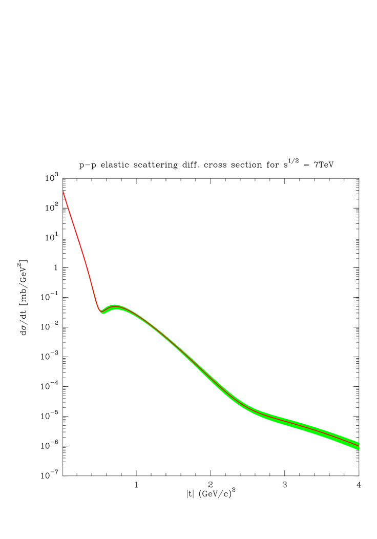
Figure 1: BSW prediction of the differential cross section versus $|t|$ for $\sqrt{s}=7\mbox{TeV}$, uncertainties are calculated with a 68% CL.

The predicted BSW differential cross section is shown in Fig. 1 with uncertainties calculated with a 68% CL, we cannot make an exact comparison with experiment since no final data are available, qualitatively we observe that the BSW differential cross section is above TOTEM at the second maximum by a factor around 1.7.

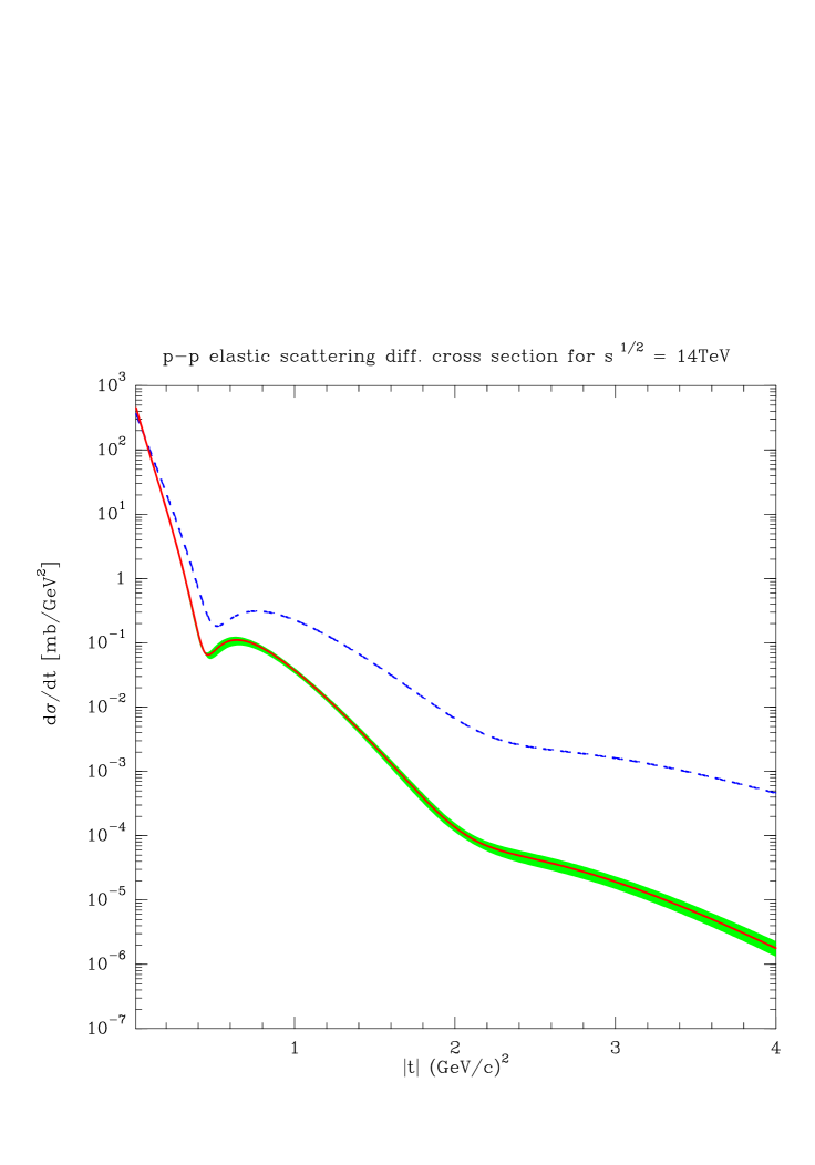
Figure 7: The elastic differential cross section versus $|t|$ for $\sqrt{s}=14\mbox{TeV}$ calculated using Eq. (46) dashed curve, BSW solid curve.

In view of a future experiment at $\sqrt{s}=14\mbox{TeV}$ we give our predictions: $\sigma_{tot}=103.63\pm 1.0$ mb, $\rho=0.122\pm 0.02$, the slope B near the forward direction gives 20.15GeV^-2, $\sigma_{el}=28.76\pm 0.2$ mb, and the elastic differential cross section is shown in Fig. 7 where $|t_{dip}|=0.45$ GeV².

4 The evaluation of $F(x_{\perp})$ and its consequences

The purpose of this section is to find the exact expression of $F(x_{\perp})$, entering in Eq. (7), in order to determine the most relevant region in $x_{\perp}$ for the calculation of the asymptotic limit of $\mathcal{M}(s,\Delta)$, for large $s$.
Noting that $\tilde{F}$ depends only on $\Delta^{2}$, the Fourier transform that defines $F$ simplifies to an integral over one variable, so that we have

$$F(x_{\perp})=\int_{0}^{\infty}d\Delta\,\Delta\,\tilde{F}(-\Delta^{2})J_{0}(x_{\perp}\Delta)~{},$$ (10)

where $J_{0}$ denotes the Bessel function of zero order. From Eq. (8), we have explicitely

$$\tilde{F}(-\Delta^{2})=f\,\frac{1}{(1+\Delta^{2}/m_{1}^{2})^{2}(1+\Delta^{2}/m_{2}^{2})^{2}}\frac{a^{2}-\Delta^{2}}{a^{2}+\Delta^{2}}~{},$$ (11)

which is a rational fraction, symmetric in $m_{1},m_{2}$, whose decomposition into simple elements, allows the direct calculation of $F(x_{\perp})$. As expected, the final result can be expressed in terms of modified Bessel functions $K_{0}$ and $K_{1}$. We have the decomposition

$$F(x_{\perp})=F_{1}(x_{\perp})+F_{2}(x_{\perp})+F_{3}(x_{\perp})~{},$$ (12)

where

$$F_{1}(x_{\perp}) = \frac{fm_{1}^{4}m_{2}^{4}}{2(m_{2}^{2}-m_{1}^{2})^{3}}\bigg{\{}\frac{m_{2}^{2}-m_{1}^{2}}{m_{1}^{2}}\,\frac{a^{2}+m_{1}^{2}}{a^{2}-m_{1}^{2}}(m_{1}x_{\perp})K_{1}(m_{1}x_{\perp})$$ (13)

$$-4\left[\frac{a^{2}+m_{1}^{2}}{a^{2}-m_{1}^{2}}+\frac{(m_{2}^{2}-m_{1}^{2})a^{2}}{(a^{2}-m_{1}^{2})^{2}}\right]K_{0}(m_{1}x_{\perp})\bigg{\}}$$

$$F_{2}(x_{\perp}) = \frac{fm_{1}^{4}m_{2}^{4}}{2(m_{2}^{2}-m_{1}^{2})^{3}}\bigg{\{}\frac{m_{2}^{2}-m_{1}^{2}}{m_{2}^{2}}\,\frac{a^{2}+m_{2}^{2}}{a^{2}-m_{2}^{2}}(m_{2}x_{\perp})K_{1}(m_{2}x_{\perp})$$ (14)

$$+4\left[\frac{a^{2}+m_{2}^{2}}{a^{2}-m_{2}^{2}}-\frac{(m_{2}^{2}-m_{1}^{2})a^{2}}{(a^{2}-m_{2}^{2})^{2}}\right]K_{0}(m_{2}x_{\perp})\bigg{\}}$$

$$F_{3}(x_{\perp}) = \frac{2fm_{1}^{4}m_{2}^{4}a^{2}}{(a^{2}-m_{1}^{2})^{2}(a^{2}-m_{2}^{2})^{2}}K_{0}(ax_{\perp})~{},$$ (15)

which is clearly symmetric in $m_{1},m_{2}$. The arguments of the modified Bessel functions $K_{1}$ and $K_{0}$ are $m_{1}x_{\perp}$ for $F_{1}$, while $m_{2}x_{\perp}$ for $F_{2}$ and $ax_{\perp}$ for $F_{3}$. The function $F$ is real, positive, bounded, and monotonically decreasing toward 0 as $x_{\perp}$ increases without bound. Because $\text{Re}\mathcal{S}$ is large and positive for large values of $\ln s$, the only contribution to $\mathcal{M}$ comes from $x_{\perp}$ fairly near $\ln s$, so that the large argument asymptotic expressions for the modified Bessel functions are applicable. Since as seen from Table 1, $m_{1}<m_{2}<a$, $F_{2}$ and $F_{3}$ are exponentially smaller than $F_{1}$, only $F_{1}$ contributes to the asymptotic behavior of $\mathcal{M}(s,\Delta)$. For the moment we keep the exact expression for $F(x_{\perp})$, but we change variables to emphasize the role of $F_{1}$ as follows. Let us define two dimensionless variables

$$x=m_{1}x_{\perp},$$ (16)

$$\alpha=\Delta/m_{1}.$$ (17)

With this change of variables, Eq. (7) becomes

$$\mathcal{M}(s,\Delta)=\frac{is}{m_{1}^{2}}\int_{0}^{\infty}dx\,x\,J_{0}(\alpha x)\left[1-e^{-\mathcal{S}(s)\hat{F}(x)}\right]~{},$$ (18)

where $\hat{F}(x)=\hat{F}_{1}(x)+\hat{F}_{2}(x)+\hat{F}_{3}(x)$ and $\hat{F}_{j}(x)\equiv F_{j}(x/m_{1})=F_{j}(x_{\perp})$, for $j=1,2,3$. We note that for $x\gg 1$ the asymptotic representation of $\hat{F}$, implied by Eqs. (13) and (16) and the asymptotic representation of the modified Bessel function [13], is

$$\hat{F}(x) \sim \frac{fm_{1}^{2}m_{2}^{4}(a^{2}+m_{1}^{2})}{2(m_{2}^{2}-m_{1}^{2})^{2}(a^{2}-m_{1}^{2})}x\,K_{1}(x)$$ (19)

$$\sim b\sqrt{x}\,e^{-x},$$ (20)

where $b$ is the real coefficient

$$b=\frac{fm_{1}^{2}m_{2}^{4}(a^{2}+m_{1}^{2})}{2(m_{2}^{2}-m_{1}^{2})^{2}(a^{2}-m_{1}^{2})}\sqrt{\pi/2}.$$ (21)

5 High-energy asymptotic behavior

Some additional approximations make it possible to obtain an expression of the scattering amplitude in the high energy limit. The integrand of the integral in Eq. (7) is complex. From the definition of $\mathcal{S}(s)$ in Eq. (4) and the explicit expression in Eq. (6), we notice that for sufficiently high values of $s$, namely

$$\ln s\gg\pi~{},$$ (22)

the second denominator in Eq. (6) can be approximated by the first denominator, so that

$$\mathcal{S}(s)\sim\frac{2s^{c}}{(\ln s)^{c^{\prime}}}\cos\left(\frac{\pi c}{2}\right)e^{-\frac{1}{2}i\pi c}~{}.$$ (23)

Thus the phase of $S(s)$ is found to be a constant, namely, $-\frac{1}{2}\pi c\approx-0.26$ and when $\ln s$ is large one has

$$\text{Re}\mathcal{S}(s)>\text{Im}\mathcal{S}\gg 1.$$ (24)

The function $\hat{F}(x)$ is positive for all real $x$ and decreasing exponentially with large $x$ as stated in Eq.(20). Because of these properties of $\hat{F}(x)$ and the large value of $\text{Re}\mathcal{S}$, the opacity is essentially 1 for values of $x$, well below a transition value, and drops exponentially to zero as $x$ increases well above this transition value. From this, it follows that the asymptotic representation of the scattering amplitude can be obtained by replacing $\hat{F}(x)$ by $\hat{F}(z_{0})e^{-(x-z_{0})}$, where $z_{0}$ is a complex transition value chosen in such a way to make $\mathcal{S}(s)\hat{F}(z_{0})$ real and of order 1.
By means of a translation in the complex plane from $x$ to $x^{\prime}=x-z_{0}$, the scattering amplitude of Eq. (18) becomes asymptotically

$$\mathcal{M}(s,\Delta) \sim \frac{is}{m_{1}^{2}}\int_{-z_{0}}^{\infty}dx^{\prime}(x^{\prime}+z_{0})J_{0}[\alpha(x^{\prime}+z_{0})]\left[1-e^{-\mathcal{S}(s)\hat{F}(z_{0})e^{-x^{\prime}}}\right]$$ (25)

$$= \frac{is}{m_{1}^{2}}\left[\int_{-z_{0}}^{0}dx^{\prime}(x^{\prime}+z_{0})J_{0}[\alpha(x^{\prime}+z_{0})]+A(s,z_{0})\right]$$ (26)

$$= \frac{is}{m_{1}^{2}}\left[\frac{z_{0}}{\alpha}J_{1}(\alpha z_{0})+A(s,z_{0})\right]~{},$$ (27)

where we define

$$A(s,z_{0}) = \int_{0}^{\infty}dx^{\prime}(x^{\prime}+z_{0})J_{0}[\alpha(x^{\prime}+z_{0})]\left[1-e^{-\mathcal{S}(s)\hat{F}(z_{0})e^{-x^{\prime}}}\right]$$ (28)

$$-\int_{-z_{0}}^{0}dx^{\prime}(x^{\prime}+z_{0})J_{0}[\alpha(x^{\prime}+z_{0})]e^{-\mathcal{S}(s)\hat{F}(z_{0})e^{-x^{\prime}}}.$$

It remains to determine $z_{0}$ and then to evaluate the asymptotic representation of $A(s,z_{0})$. In order to find $z_{0}$ we use the following relation derived in Appendix A (see Eq. (A.7))

$$0=\int_{0}^{\infty}dx\left[1-e^{\displaystyle{-e^{-\gamma}e^{-x}}}\right]-\int_{-\infty}^{0}dx\,e^{\displaystyle{-e^{-\gamma}e^{-x}}}~{},$$ (29)

which suggests defining $z_{0}$ as solution of the equation

$$\mathcal{S}(s)\hat{F}(z_{0})=e^{-\gamma}~{},$$ (30)

where $\gamma\approx 0.5772$ is the Euler’s constant. While $z_{0}$, as a function of $s$, is best obtained by solving Eq. (30) numerically, one can see its approximate value by using the asymptotic representation for $\hat{F}$, so that

$$\mathcal{S}(s)b\sqrt{z_{0}}\,e^{-z_{0}}\approx e^{-\gamma}.$$ (31)

By taking logarithms one finds

$$z_{0}\approx\ln[b\sqrt{z_{0}}\mathcal{S}(s)]+\gamma,$$ (32)

showing how $\text{Re}\,z_{0}$ grows with $\text{Re}\,\ln[\mathcal{S}(s)]$ and how $\text{Im}\,z_{0}=\arg(\mathcal{S}(s))$ approaches $-0.26$, as $\ln s$ becomes very large (see Fig. 1). Then the fact that $\text{Re}\,z_{0}$ is large can be used twice. First, in Eq. (28), one can safely replace the lower limit $-z_{0}$ in one of the integrals by $-\infty$, so that

$$A(s,z_{0}) \sim \int_{0}^{\infty}dx(x+z_{0})J_{0}[\alpha(x+z_{0})]\left[1-e^{-e^{-(x+\gamma)}}\right]$$ (33)

$$-\int_{-\infty}^{0}dx(x+z_{0})J_{0}[\alpha(x+z_{0})]e^{-e^{-(x+\gamma)}}.$$

Secondly, since the important regions of integration are where $x$ is of the order of $1$, to determine the leading order behavior of the scattering amplitude it suffices to replace the factors $(x+z_{0})$ by $z_{0}$, so Eq. (33) reduces to

$$A(s,z_{0}) \sim z_{0}\bigg{\{}\int_{0}^{\infty}dx\,J_{0}[\alpha(x+z_{0})]\left[1-e^{-e^{-(x+\gamma)}}\right]$$ (34)

$$-\int_{-\infty}^{0}dx\,J_{0}[\alpha(x+z_{0})]e^{-e^{-(x+\gamma)}}\bigg{\}}.$$

To determine the asymptotic behavior of $A(s,z_{0})$, we have to study the Bessel function which depends upon the parameter $\alpha$, and there are two regions to consider.

i) Small $\alpha$ region
By assuming that $\alpha$ is small, but not $\alpha z_{0}$, we keep only the first three terms of the Taylor series to obtain:

$$J_{0}[\alpha(z_{0}+x)]=J_{0}(\alpha z_{0})-\alpha xJ_{1}(\alpha z_{0})-\frac{(\alpha x)^{2}}{2}J_{0}(\alpha z_{0})+\text{higher order terms}.$$ (35)

By substituting Eq. (35) into Eq. (34), one obtains after some integration by parts

$$A(s,z_{0}) \sim z_{0}\bigg{[}\mathcal{I}_{1}(e^{-\gamma})J_{0}(\alpha z_{0})-\frac{\alpha}{2}\mathcal{I}_{2}(e^{-\gamma})J_{1}(\alpha z_{0})$$ (36)

$$-\frac{\alpha^{2}}{6}\mathcal{I}_{3}(e^{-\gamma})J_{0}(\alpha z_{0})\bigg{]}$$

$$= -z_{0}\left[\frac{\pi^{2}\alpha}{12}J_{1}(\alpha z_{0})+\frac{\alpha^{2}}{3}\zeta(3)J_{0}(\alpha z_{0})\right],$$

where the $\mathcal{I}_{n}$ are defined in Appendix A and $\zeta$ is the Riemann Zeta function, and therefore $\zeta(3)\approx 1.2021$.

ii) Large $\alpha$ region
In this region the large argument asymptotic expansion of the Bessel function [13] allows one to write, for large $|z_{0}|$ and the contributing values of $x$ which are $O(1)$,

$$J_{0}[\alpha(z_{0}+x)] = \sqrt{\frac{2}{\pi z_{0}}}\cos[\alpha(z_{0}+x-\pi/4)]+\text{higher order terms}$$ (37)

$$= \frac{1}{\sqrt{2\pi z_{0}}}\left[e^{i\alpha(z_{0}-\pi/4)}e^{i\alpha x}+e^{-i\alpha(z_{0}-\pi/4)}e^{-i\alpha x}\right]+....$$

By substituting Eq. (37) into Eq. (34), this yields for this region of $\alpha$

$$A(s,z_{0}) \sim \sqrt{\frac{z_{0}}{2\pi}}\left[e^{i(\alpha z_{0}-\pi/4)}\mathcal{J}(i\alpha)+e^{-i(\alpha z_{0}-\pi/4)}\mathcal{J}(-i\alpha)\right]$$

$$= z_{0}\sqrt{\frac{2}{\pi z_{0}}}\left[\cos(\alpha z_{0}-\pi/4)\text{Re}\mathcal{J}(i\alpha)-\sin(\alpha z_{0}-\pi/4)\text{Im}\mathcal{J}(i\alpha)\right],$$

where it follows from Eq. (A.11) of Appendix A that

$$\mathcal{J}(i\alpha)=\frac{i}{\alpha}-e^{-i\gamma\alpha}\Gamma(-i\alpha)~{}.$$ (39)

Comparison with Eq. (37) and the similar expression for $J_{1}$ shows that to leading order, this result can be expressed in terms of Bessel functions

$$A(s,z_{0})\sim z_{0}\left[J_{0}(\alpha z_{0})\text{Re}\mathcal{J}(i\alpha)-J_{1}(\alpha z_{0})\text{Im}\mathcal{J}(i\alpha)\right]$$

$$=-z_{0}\!\!\left[\!\left(\frac{1}{\alpha}+\text{Im}\left[e^{i\gamma\alpha}\Gamma(i\alpha)\right]\right)J_{1}(\alpha z_{0})\!\!+\!\!\left(\text{Re}\left[e^{i\gamma\alpha}\Gamma(i\alpha)\right]\right)J_{0}(\alpha z_{0})\!\right].$$ (40)

iii) Uniform approximation
Expanding the Gamma function for small $\alpha$, one obtains Eq. (36), showing that Eq. (40) gives a uniform approximation including both regions of the parameter $\alpha$. Then from Eq. (27) it follows that for $0\leq\alpha\ll|z_{0}|$, the asymptotic representation of the scattering amplitude is

$$\mathcal{M}(s,\Delta)\sim-\frac{isz_{0}}{m_{1}^{2}}\left\{\left[\text{Im}(e^{i\gamma\alpha}\Gamma(i\alpha))\right]J_{1}(\alpha z_{0})+\left[\text{Re}(e^{i\gamma\alpha}\Gamma(i\alpha))\right]J_{0}(\alpha z_{0})\right\}~{}.$$ (41)

6 Numerical results

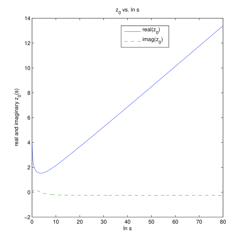
Figure 2: The real and imaginary parts of $z_{0}(s)$ as a function of the energy, obtained by solving numerically Eq. (30).

In this section we present some numerical results to illustrate the asymptotic formulas obtained on the physical quantities of interest for different energy values. First let us come back to the determination of the complex parameter $z_{0}(s)$ which plays an essential role in the solution of the high energy asymptotic behavior of the scattering amplitude. As we said earlier, $z_{0}$ is obtained by solving numerically Eq. (30) and the results are shown on Fig. 2, for $\text{Re}z_{0}(s)$ and $\text{Im}z_{0}(s)$, versus $\ln{(s)}$. As expected, $\text{Re}z_{0}(s)$ rises rapidly with $\ln{(s)}$, whereas $\text{Im}z_{0}(s)$ remains small and almost energy independent. It is worth noting that the asymptotic regime requires the validity of Eq. (22), for example for $\ln{(s)}=10\pi$, corresponding to the center-of energy $\sqrt{s}$ of about 6000TeV.

The asymptotic representation of the forward scattering amplitude is obtained from Eq. (41) by taking the limit as $\alpha\rightarrow 0$

$$\mathcal{M}(s,0)\sim\frac{isz_{0}^{2}}{2m_{1}^{2}}~{}.$$ (42)

From this formula we calculate the ratio of the real to the imaginary parts of the forward amplitude defined as

$$\rho(s)=\frac{\text{Re}\mathcal{M}(s,0)}{\text{Im}\mathcal{M}(s,0)}~{}.$$ (43)

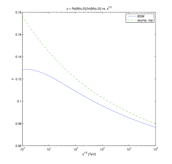
Figure 3: The ratio of the real to the imaginary parts of the forward amplitude versus $\sqrt{s}$. Top using Eq. (42) and bottom using Eq. (45) dashed curves, BSW solid curves.

In Fig. 3 (top) we display this result compared to the exact BSW result. We see that $\rho(s)$ decreases for increasing energy, in agreement with the expectation that $\rho(s)\to 0$, when $s$ goes to infinity.
The total cross section is obtained from the optical theorem as follows,

$$\sigma_{\text{tot}}=\frac{4\pi}{s}\text{Im}\mathcal{M}(s,0),$$ (44)

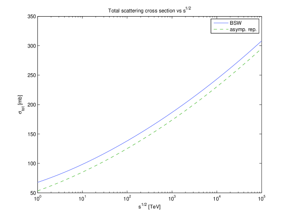
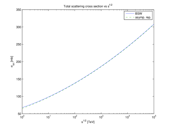
Figure 4: The total cross section $\sigma_{tot}$ versus $\sqrt{s}$. Top using Eq. (42) and bottom using Eq. (45) dashed curves, BSW solid curves.

and we recall that $\mathcal{M}(s,0)$ is dimensionless. It is plotted in Fig 4 (top) compared to the exact BSW result.
In Figs. 3, 4 (top), a gap can be noticed between the asymptotic representation and the BSW model. The gaps extend to the end of the plotted energy range of $s^{1/2}=10^{5}$ TeV, where $\ln{(s)}\approx 37$. To show that the asymptotic representation actually approaches BSW at sufficiently large values of $\ln s$, we carried out the first three terms of an asymptotic expansion to obtain

$$\mathcal{M}(s,0)\sim\frac{is}{2m_{1}^{2}}\left(z_{0}^{2}+\frac{\pi^{2}}{6}\right)+O(1/z_{0})~{}.$$ (45)

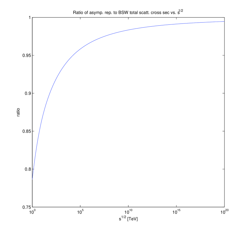
Figure 5: The ratio of the leading order of the asymptotic representation to the exact BSW result, versus the energy.

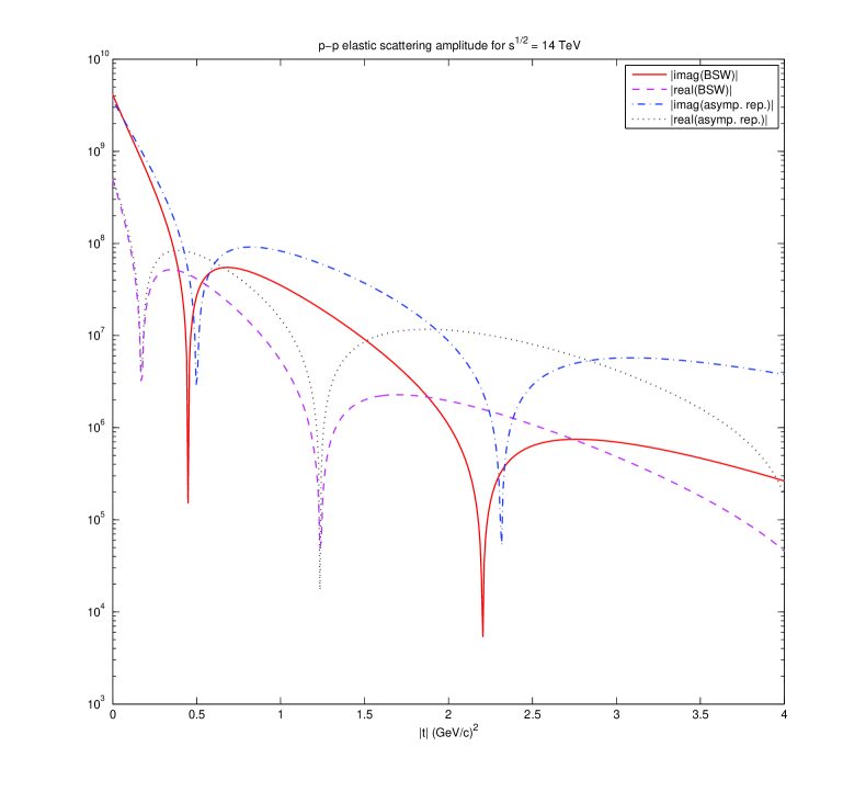
Figure 6: The absolute value of the real and imaginary parts of the elastic scattering amplitude, as a function of $|t|$ for $\sqrt{s}=14\text{TeV}$, for the exact BSW result (Real: dashed, Im: solid) and the asymptotic representation (Real: dotted, Im: dash-dotted).

With this expression in place of (42), the gaps largely close, as seen in Figs. 3, 4 (bottom). This shows indeed that the gaps visible in Figs. 3, 4 (top) are due to the neglect of non-leading terms in the asymptotic representation. In Fig. 5 we display the ratio of the leading order of the asymptotic representation to the exact BSW result, which goes to 1 for very, very large $s$, as expected. Now let us move from the forward direction to look at the behavior of the real and imaginary parts of the scattering amplitude as functions of $t$. For $\sqrt{s}=14\text{TeV}$, Fig. 6 displays the exact BSW amplitude along with its asymptotic representation. In both cases the imaginary part dominates the real part and its zeros will produce oscillations in the differential cross section, as shown in Fig. 7. The differential cross section is given by

$$\frac{d\sigma}{dt}=\frac{\pi}{s^{2}}|\mathcal{M}(s,\Delta)|^{2}\,,$$ (46)

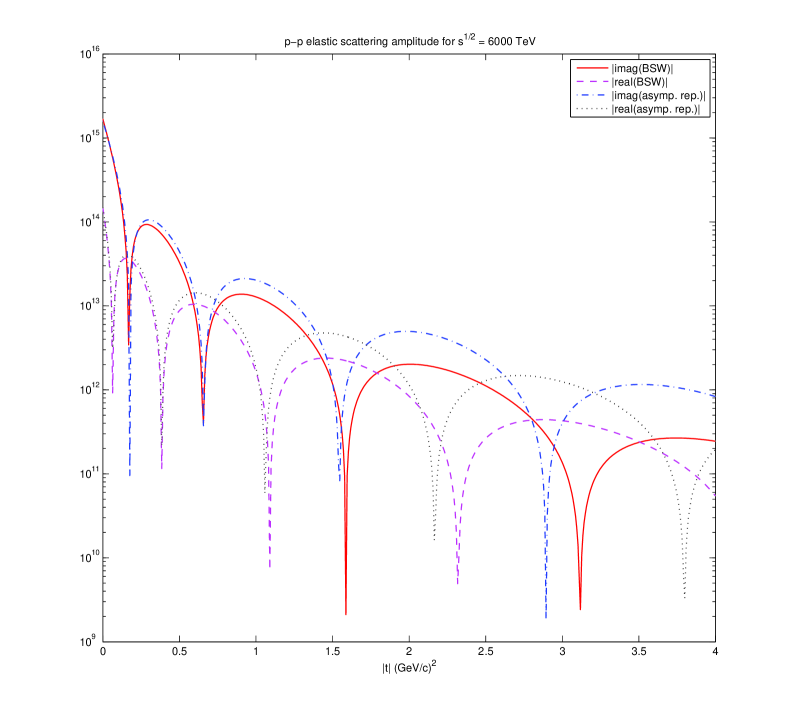
Figure 8: The absolute value of the real and imaginary parts of the elastic scattering amplitude, as a function of $|t|$ for $\sqrt{s}=6000\text{TeV}$, , for the exact BSW result (Real: dashed, Im: solid) and the asymptotic representation (Real: dotted, Im: dash-dotted).

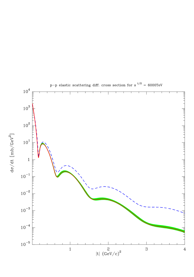
Figure 9: The elastic differential cross section calculated using Eq. (46) dashed curve, BSW solid curve.

where for the asymptotic representation one uses Eq. (41). For both the BSW amplitude and its asymptotic representation, the real part has a local maximum near each zero of the imaginary part, and vice versa. When the maximum of the real part near a zero of the imaginary part is relatively low, as in the case near $|t|=0.5\text{GeV}^{2}$, one gets a sharp dip, but if not, like near $|t|=2\text{GeV}^{2}$, one gets instead a smooth oscillation. Clearly the asymptotic result is larger than the exact BSW result, except near the diffraction peak, where they are hardly distinguishable. At a much higher energy $\sqrt{s}=6000\text{TeV}$, the number of zeros increases, as shown in Fig. 8 and the low maximum of the real part near the zero of the imaginary part around $|t|=0.2\text{GeV}^{2}$, generates a very sharp dip in the cross section, as seen in Fig. 9, followed by another dip and some smooth oscillations.

7 Concluding remarks

After recalling the basic features of the BSW model, we have presented our predictions for the LHC energies and compared them with preliminary results from TOTEM. We have obtained the asymptotic representation of the BSW model in terms of a simple formula. The existence of several zeros for both the real and the imaginary parts of the scattering amplitude, generates oscillations in the differential cross section. The exact BSW result tends to coincide with this asymptotic representation, as the energy increases. This is even more striking near the forward direction, in particular for the diffraction peak of the differential cross section. In connection with this, let us mention now the following interesting feature of the asymptotic representation. A unitarity upper bound for the imaginary part of the scattering amplitude for very high energy and small momentum transfers was derived a long time ago by Singh and Roy [14]. It reads

$$\frac{\text{Im}\mathcal{M}(s,t)}{\text{Im}\mathcal{M}(s,0)}\leq\frac{2J_{1}(\sqrt{r})}{\sqrt{r}},~{}~{}~{}~{}~{}~{}~{}~{}\text{if}~{}~{}r<3.46~{},$$ (47)

with $r=|t|\sigma_{tot}(s)/4\pi$. For $s$ very large, from Eq. (41), we see that this variable is simply $\eta=\alpha\text{Re}z_{0}$. The ratio $\text{Im}\mathcal{M}(s,t)\over\text{Im}\mathcal{M}(s,0)$ has been plotted in Fig. 10, versus $\eta$, for $\sqrt{s}=14\text{TeV}$. We compare the exact BSW result with the asymptotic representation and also with the Singh-Roy upper bound limit $s\to\infty$. We observe that the validity of the bound is, indeed, limited to $\eta<3.46$. Fig. 11 displays the situation at $\sqrt{s}=6000\text{TeV}$ and in this case the upper bound, whose validity is still limited to the diffraction peak, becomes much closer to the other two curves.

Acknowledgments We thank J.M Richard for drawing our attention to the old bound of Singh and Roy. One of us (T.T.W) is greatly indebted to the CERN Theory Group for their hospitality.

Appendix A Appendix

For the small $\alpha$ region, we define

$$\mathcal{I}_{n}(\beta) = \int_{-\infty}^{\infty}dx\,x^{n}\,\frac{d\;}{dx}e^{\displaystyle{-\beta e^{-x}}}$$ (A.1)

$$= \beta\int_{-\infty}^{\infty}dx\,x^{n}\,e^{-x}e^{\displaystyle{-\beta e^{-x}}}$$ (A.2)

$$= \int_{0}^{\infty}dt[\ln(\beta/t)]^{n}e^{-t}$$ (A.3)

$$= \left[\left(\ln\beta-\frac{d}{d\nu}\right)^{n}\int_{0}^{\infty}dt\,t^{\nu}e^{-t}\right]\bigg{|}_{\nu=0}$$ (A.4)

$$= \left[\left(\ln\beta-\frac{d}{d\nu}\right)^{n}\Gamma(1+\nu)\right]\bigg{|}_{\nu=0},$$ (A.5)

where $t=\beta e^{-x}$ and $\Gamma$ is the Gamma function. The results for $n=0,1,2,3$ are given in Table 2. Here $\gamma\approx 0.5772$ is the Euler’s constant and $\zeta$ is the Riemann Zeta function. The choice of $z_{0}$ made in Eq. (30) draws on the fact that

$$\mathcal{I}_{1}(e^{-\gamma})=-\gamma+\gamma=0,$$ (A.6)

hence Eq. (29) follows as

$$0 = \int_{-\infty}^{0}dx\,x\,\frac{d\;}{dx}e^{\displaystyle{-e^{-\gamma}e^{-x}}}-\int_{0}^{\infty}dx\,x\,\frac{d\;}{dx}\left[1-e^{\displaystyle{-e^{-\gamma}e^{-x}}}\right]$$ (A.7)

$$= \int_{0}^{\infty}dx\left[1-e^{\displaystyle{-e^{-\gamma}e^{-x}}}\right]-\int_{-\infty}^{0}dx\,e^{\displaystyle{-e^{-\gamma}e^{-x}}}~{}.$$ (A.8)

For the large $\alpha$ region one needs $\mathcal{J}(i\alpha)$ and $\mathcal{J}(-i\alpha)$ where we define

$$\mathcal{J}(i\alpha) \ = \int_{0}^{\infty}dx\,e^{i\alpha x}\left[1-e^{\displaystyle{-e^{-(x+\gamma)}}}\right]-\int_{-\infty}^{0}dx\,e^{i\alpha x}e^{\displaystyle{-e^{-(x+\gamma)}}}$$ (A.9)

$$= \frac{1}{i\alpha}\left[-1+\int_{-\infty}^{\infty}e^{i\alpha x}\frac{d\;}{dx}e^{\displaystyle{e^{-(x+\gamma}}}\right]$$ (A.10)

$$= \frac{1}{i\alpha}\left[-1+e^{-i\gamma\alpha}\Gamma(1-i\alpha)\right]~{}.$$ (A.11)

From Eq. (A.11) and the properties of the Gamma function [15], it follows that $\mathcal{J}(-i\alpha)$ is the complex conjugate of $\mathcal{J}(i\alpha)$.
For small values of $\alpha$ one finds

$$\mathcal{J}(i\alpha)\approx\frac{i\pi^{2}\alpha}{12}-\frac{\alpha^{2}}{3}\zeta(3)~{}.$$ (A.12)

$n$	$\mathcal{I}_{n}(\beta)$
$0$	$1$
$1$	$\ln\beta+\gamma$
$2$	$(\ln\beta+\gamma)^{2}+\pi^{2}/6$
$3$	$(\ln\beta+\gamma)^{3}+\frac{\pi^{2}}{2}(\ln\beta+\gamma)+2\zeta(3)$

Table 2: Values of $\mathcal{I}_{n}(\beta)$

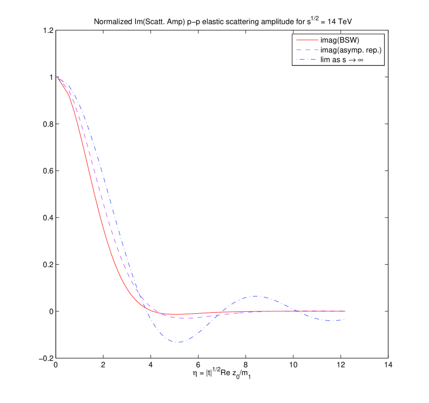
Figure 10: The normalized imaginary part of the elastic scattering amplitude for $\sqrt{s}=14\text{TeV}$. BSW solid, asymptotic dashed, lim$~{}s\rightarrow\infty$ dash-dotted.

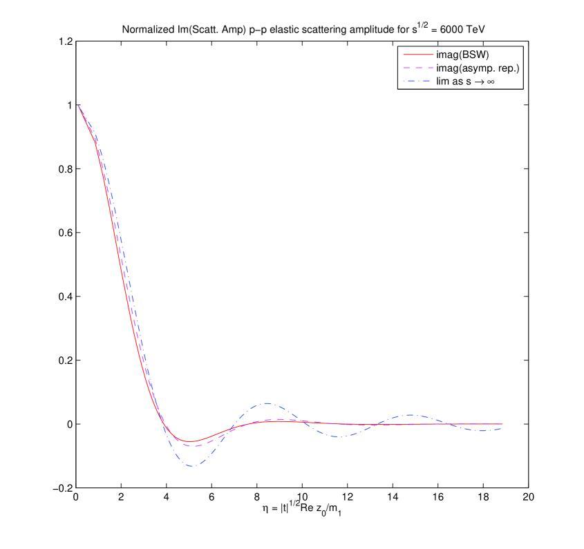
Figure 11: The normalized imaginary part of the elastic scattering amplitude for $\sqrt{s}=6000\text{TeV}$ (same legend as in Fig. 10).

References

- [1] H. Cheng and T. T. Wu, Phys. Rev. Lett. 24, 1456 (1970) (See also H. Cheng and T. T. Wu, Expanding Protons: Scattering at High Energies (MIT Press, Cambridge, MA, 1987)).
- [2] C. Bourrely, J. Soffer, and T. T. Wu, Phys. Rev. D 19, 3249 (1979).
- [3] C. Bourrely, J. Soffer, and T. T. Wu, Nucl. Phys. B 247, 15 (1984).
- [4] C. Bourrely, J. Soffer, and T. T. Wu, Eur. Phys. J. C 28, 97 (2003).
- [5] M. M. Block and F. Halzen, Phys. Rev. D 83 (2011) 077901.
- [6] M. M. Islam et al., Int. J. Mod. Phys. A 21 (2006) 1.
- [7] J. Kašpar et al., Nucl. Phys. B 843 (2011) 84.
- [8] P.A.S. Carvalho et al., Eur. Phys. J. C 39 (2005) 359.
- [9] V. Petrov et al., Eur. Phys. J. C 28 (2003) 525.
- [10] G. Antchev et al., Eur. Phys. Lett. 95 (2011) 41001, 96 (2011) 21002.
- [11] ATLAS-ALFA collaboration, CERN-LHCC-2004-010, CERN-LHCC-2008-004.
- [12] C. Bourrely, J. Soffer, and T. T. Wu, Eur. Phys. J. C 71, 1061 (2011).
- [13] A. Erdélyi, ed., Higher Transcendental Functions, Vol II (McGraw-Hill Book Co., New York, 1953).
- [14] V. Singh and S.M. Roy, Phys. Rev. D 1, 2638 (1970).
- [15] A. Erdélyi, ed., Higher Transcendental Functions, Vol I (McGraw-Hill Book Co., New York, 1953).