Unveiling hidden properties of young star clusters: differential reddening, star-formation spread and binary fraction

Abstract

Context. Usually, important parameters of young, low-mass star clusters are very difficult to obtain by means of photometry, especially when differential reddening and/or binaries occur in large amounts.

Aims. We present a semi-analytical approach ($ASA_{min}$) that, applied to the Hess diagram of a young star cluster, is able to retrieve the values of mass, age, star-formation spread, distance modulus, foreground and differential reddening, and binary fraction.

Methods. The global optimisation method known as adaptive simulated annealing (ASA) is used to minimise the residuals between the observed and simulated Hess diagrams of a star cluster. The simulations are realistic and take the most relevant parameters of young clusters into account. Important features of the simulations are: a normal (Gaussian) differential reddening distribution, a time-decreasing star-formation rate, the unresolved binaries, and the smearing effect produced by photometric uncertainties on Hess diagrams. Free parameters are: cluster mass, age, distance modulus, star-formation spread, foreground and differential reddening, and binary fraction.

Results. Tests with model clusters built with parameters spanning a broad range of values show that $ASA_{min}$ retrieves the input values with a high precision for cluster mass, distance modulus and foreground reddening, but somewhat lower for the remaining parameters. Given the statistical nature of the simulations, several runs should be performed to obtain significant convergence patterns. Specifically, we find that the retrieved (absolute minimum) parameters converge to mean values with a low dispersion as the Hess residuals decrease. When applied to actual young clusters, the retrieved parameters follow convergence patterns similar to the models. We show how the stochasticity associated with the early phases may affect the results, especially in low-mass clusters. This effect can be minimised by averaging out several twin clusters in the simulated Hess diagrams.

Conclusions. Even for low-mass star clusters, $ASA_{min}$ is sensitive to the values of cluster mass, age, distance modulus, star-formation spread, foreground and differential reddening and, to a lesser degree, binary fraction. Compared with simpler approaches, the inclusion of binaries, a decaying star-formation rate and a normally distributed differential reddening, appear to yield more constrained parameters, especially the mass, age and distance from the Sun. A robust determination of cluster parameters may have a positive impact on many fields. For instance, age, mass and binary fraction are important for establishing the dynamical state of a cluster, or deriving a more precise star-formation rate in the Galaxy.

1 Introduction

Several events occurring on short timescales combine to make the first few $10^{7}$ yr the most critical period in a star cluster’s life, especially for the poorly-populated embedded clusters (ECs). Driven mainly by the impulsive removal of the parental molecular gas by supernovae and massive-star winds, the rapid and deep changes in the cluster internal dynamics lead to the escape of varying fractions of member stars to the field. The end result is that most of the low-mass clusters are dissolved before reaching $\sim 40$ Myr of age (e.g. Tutukov 1978; Goodwin & Bastian 2006). This scenario is consistent with current estimates suggesting that less than $\sim 5\%$ of the Galactic ECs dynamically evolve into gravitationally bound open clusters (e.g. Lada & Lada 2003; Bonatto & Bica 2011).

Low-mass clusters undergoing such a rapidly changing phase are usually characterised by an under-populated main sequence (MS) and significant fractions of pre-main sequence (PMS) stars, all mixed up with a spatially non-uniform dust and gas distribution. To complicate matters, star formation within a cluster appears to extend for a period that may be comparable to the cluster age (e.g. Stauffer et al. 1997), while the MS and PMS stars may be arranged in (unknown) fractions of binaries (e.g. Weidner, Kroupa & Maschberger 2009). Besides, the vast majority of the binary pairs cannot be resolved in Colour-Magnitude Diagrams (CMDs). As a result, the CMDs of young, low-mass star clusters tend to be very difficult to interpret. And, consequently, the determination of fundamental cluster parameters (e.g. age, distance, mass, foreground and internal reddening, star-formation spread (SFS), binary fraction, etc) may be somewhat subjective and unreliable, particularly when only photometry is available to work with. Examples of clusters evolving along the early phase and characterised by such complex CMDs are abundant in the recent literature. For instance: NGC 6611 (Bonatto, Santos Jr. & Bica 2006), NGC 4755 (Bonatto et al. 2006), NGC 2244 (Bonatto & Bica 2009a), Bochum 1 (Bica, Bonatto & Dutra 2008), Pismis 5 and vdB 80 (Bonatto & Bica 2009b), Collinder 197 and vdB 92 (Bonatto & Bica 2010a).

More broadly, a robust determination of fundamental parameters of young clusters may provide important constraints for studies dealing with dynamical state and cluster dissolution time-scales (e.g. Goodwin 2009; Lamers, Baumgardt & Gieles 2010), infant mortality (e.g. Lada & Lada 2003; Goodwin & Bastian 2006), star-formation rate (SFR) in the Galaxy (e.g. Lamers & Gieles 2006; Bonatto & Bica 2011), among others.

Over the years, several approaches have been proposed to tackle the important task of finding reliable parameters of young clusters. Among these, Naylor & Jeffries (2006) employ a maximum-likelihood method to Hess diagram simulations (including binaries) to derive distances and ages. However, they do not consider differential reddening (DR), and their method appears to be more efficient for clusters older than $\sim 30$ Myr. Hillenbrand, Bauermeister & White (2008) model CMDs of star forming regions and young star clusters by means of varying star-formation histories; because of confusion between signal and noise in CMDs, only marginal evidence for moderate age spreads was found. da Rio, Gouliermis & Gennaro (2010) add DR, age spreads and PMS stars to the Naylor & Jeffries (2006) method, but adopt distance and reddening values from previous work. Stead & Hoare (2011) employ Monte Carlo to estimate the age of ECs observed with near-infrared (UKIDSS) photometry. More recently, Bonatto, Bica & Lima (2011) (hereafter Paper I) included the smearing effect of photometric uncertainties on CMDs to approach the above issue by means of brute-force. However, because of computer limitations, the binary fraction, SFS, SFR, and the shape of the DR distribution had to be taken as fixed parameters.

In summary, the problem of obtaining reliable cluster parameters clearly lacks a comprehensive method that includes most (if not all) of the relevant conditions and parameters usually associated with the early cluster phases. Here we present a semi-analytical approach that follows along this direction. Instead of relying on brute-force, we now make use of the global optimisation method known as adaptive simulated annealing (ASA, adapted from Goffe, Ferrier & Rogers 1994) to search for the set of parameters that best reproduces the photometric properties (i.e., the CMD or Hess diagram) of a cluster. The free parameters are the apparent distance modulus, foreground reddening, cluster mass, age, SFS, binary fraction, and DR, which are used to build the simulated Hess diagram for a given cluster. The function to be minimised by ASA is related to differences between the observed and simulated Hess diagrams. For conciseness, hereafter we will refer to our approach as $ASA_{min}$.

By explicitly including the binary fraction, SFS and the shape of the DR distribution as free parameters on a semi-analytical approach, this work supersedes the procedure highlighted in Paper I.

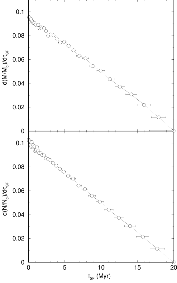
Figure 1: Top: The SFR (mass converted into stars with respect to the cluster mass) as a function of star-formation time for a cluster undergoing continuous star formation for 20 Myr. Bottom: Same as above for the number of formed stars.

The present paper is organised as follows. In Sect. 2 we discuss the relevant effects that introduce observational limitations on CMDs. In Sect. 3 we provide details on the cluster simulations. In Sect. 4 we briefly describe the $ASA_{min}$ minimisation method, test it on model clusters and discuss the strategy adopted to obtain robust parameters. In Sect. 5 we apply $ASA_{min}$ on actual young clusters, contextualise the results and discuss the low-mass cluster stochasticity. Concluding remarks are given in Sect. 6.

2 Intrinsic limitations of CMDs

Most of the problems related to obtaining reliable fundamental parameters of young clusters are illustrated in Fig. 1 of Paper I, in which a model CMD is subject to different values of distance modulus, DR and binary fraction. Clearly, when a moderate value of DR is added to the model CMD, the scatter and spread in the stellar sequences (resulting also from photometric uncertainties and binaries) tends to mask any intrinsic relationship between parameters of individual stars (e.g. the age $t_{*}$, mass $m_{*}$, magnitudes and colours) and those of the isochrones, an effect that increases significantly with distance modulus, DR amount and binary fraction.

Following Paper I, we keep working with 2MASS photometry and, in particular, with $\mbox{$J$}\times\mbox{$(J-K_{s})$}$ CMDs (the colour least affected by photometric errors and the best discriminant for PMS stars - e.g. Bonatto & Bica 2010b) and the corresponding Hess diagrams. Reddening transformations are based on the absorption relations $A_{J}/A_{V}=0.276$ and $A_{K_{S}}/A_{V}=0.118$, with $R_{V}=3.1$ (Cardelli, Clayton & Mathis 1989; Dutra, Santiago & Bica 2002). To avoid confusion between notations, we refer to the foreground reddening as $E(J-K_{s})$, where $\mbox{$E(J-K_{s})$}=0.158\mbox{$A_{V}$}$, and to the differential reddening as $\delta A_{V}$.

As shown in Paper I, the photometric uncertainties play an important role in shaping the CMD (or Hess diagram) morphology. Here we take them explicitly into account by assuming a normal (Gaussian) distribution of errors. Formally, if the magnitude (or colour) of a star is given by $\bar{x}\pm\sigma_{x}$, the probability of finding it at a specific value $x$ is given by $P(x)=\frac{1}{\sqrt{2\pi}\sigma_{x}}\,e^{{-\frac{1}{2}}\left(\frac{x-\bar{x}}{\sigma_{x}}\right)^{2}}$. Thus, for each star we compute the fraction of the magnitude and colour that falls within a given cell of the Hess diagram (i.e., the cell density). Essentially, this corresponds to the difference of the error functions computed at the cell borders. By definition, the sum of the colour and magnitude density over all Hess cells should be the number of input stars. As a compromise between CMD resolution and computational time, the Hess diagrams used in this work consist of magnitude and colour cells of size $\Delta\mbox{$J$}=0.2$ and $\Delta\mbox{$(J-K_{s})$}=0.02$, respectively.

As a photometric quality criterion, we only keep stars with errors lower than 0.2, which also serves to emulate the photometric completeness function of the observations. The effect of this restriction on the luminosity function of a model cluster containing an arbitrarily large (for statistical purposes) number of stars can be seen in Fig. 1 of Paper I. After following the steps described below for assigning the mass, magnitudes, colours and uncertainties to each star, we apply the error restriction of keeping only stars with errors $\leq 0.1$ and 0.2. Compared to the complete luminosity function, which presents a turnover at $\mbox{$J$}\approx 16.9$, the restricted functions have turnovers that smoothly shift towards brighter magnitudes.

3 A simulation recipe for young clusters

Major changes with respect to the procedures adopted in Paper I for simulating young clusters are as follows: (i) The DR is described as a normal distribution, characterised by the mean $\overline{\delta A}_{V}$ and standard deviation around the mean $\sigma(\mbox{$\delta A_{V}$})$, where both are free parameters. (ii) The SFR is a linearly decreasing function of time, which is a more realistic assumption, especially for clusters older than $\sim 10$ Myr (e.g. Belloche et al. 2011; Bate 2011 and references therein). Although somewhat arbitrary, this assumption has the advantage of requiring a single free parameter. In this case, it is just the cluster age ($t_{clu}$), which we assume as the beginning of the star-forming event. For a cluster of mass $M_{clu}$ and age $t_{clu}$, the SFR is the mass $M$ converted in stars as a function of time after the star formation start $t_{sf}$, which we express as $\frac{d\,M}{d\,t_{sf}}=\frac{2\,M_{clu}}{\mbox{$t_{clu}$}}\left(1-t_{sf}/t_{clu}\right)$. This SFR is illustrated in Fig. 1 (top panel), for a 20 Myr old cluster that has been forming stars during the same time. Equivalently, the fraction of formed stars is also a linearly decreasing function of time (bottom). (iii) The SFS timescale ($\tau_{sfs}$) is now a free parameter; instead of a fixed (and assumed to be equal to the cluster age) value, it can vary within the range $0\leq\mbox{$\tau_{sfs}$}\leq\mbox{$t_{clu}$}$. Specifically, $\tau_{sfs}$ corresponds to the difference between $t_{clu}$ and the minimum (isochrone) age compatible with the CMD stellar distribution. (iv) Binaries are expected to survive the early evolutionary phase of low-mass clusters, with the unresolved pairs being somewhat brighter and redder than the single stars, thus resulting in some broadening of the CMD stellar sequences, especially the MS (e.g. Naylor & Jeffries 2006). We include them in our simulations by means of the (free) parameter $f_{bin}$, which measures the fraction of unresolved binaries in a CMD. According to this definition, a CMD with $N_{CMD}$ detections and characterised by the binary fraction $f_{bin}$, would have a number of individual stars expressed as $N_{*}=(1+\mbox{$f_{bin}$})N_{CMD}$. As an additional assumption, binaries are formed by pairing stars with the closest ages, regardless of the individual masses. This gives rise to a secondary to primary stellar mass-ratio ($q=m_{s}/m_{p}$) that smoothly increases from very-low values up to $q\approx 0.25$, and decreases for higher values of $q$ (Fig. 1 of Paper I).

Thus, to simulate the CMD of a cluster on a given photometric system we: (i) Start with an artificial cluster of mass $M_{clu}$, age $t_{clu}$, SFS timescale $\tau_{sfs}$, apparent distance modulus $(m-M)_{J}$, foreground reddening $E(J-K_{s})$, mean DR $\overline{\delta A}_{V}$ and standard deviation $\sigma(\mbox{$\delta A_{V}$})$, and binary fraction $f_{bin}$. (ii) Assign each star an age according to $\mbox{$t_{clu}$}-\mbox{$\tau_{sfs}$}\leq\mbox{$t_{*}$}\leq\mbox{$t_{clu}$}$, with a probability following a linearly decreasing age distribution (Fig. 1). (iii) Select the individual stellar masses ($m_{*}$) by randomly taking values from Kroupa (2001) mass function (with the upper mass value consistent with the age), until $\sum_{i}\mbox{$m_{*}$}_{i}=\mbox{$M_{clu}$}$. (iv) Compute the magnitudes and colours of each star according to $t_{*}$ and $m_{*}$, and the mass to light relations taken from the isochrone corresponding to $t_{*}$. (v) Form the (unresolved) binary pairs according to $f_{bin}$ and compute their magnitudes and colours. (vi) For each star, randomly compute DR from a normal distribution characterised by the mean $\overline{\delta A}_{V}$ and standard deviation $\sigma(\mbox{$\delta A_{V}$})$. (vii) Apply shifts in colour and magnitude according to the values of $E(J-K_{s})$ and $(m-M)_{J}$. (viii) Assign each artificial star a photometric uncertainty based on the average 2MASS errors and magnitude relationship. (ix) For more realistic representativeness, add some photometric noise to the stars. This step is taken to minimise the probability of stars with the same mass having exactly the same observed magnitude, colour, and uncertainty in the CMD. To do this, consider a star (of mass $m_{*}$ and age $t_{*}$) with an intrinsic (i.e., measured from the corresponding isochrone) magnitude $\overline{mag}$ and assigned uncertainty $\sigma_{mag}$. The noise-added magnitude $mag$ is then randomly computed from a normal distribution with a mean $\overline{mag}$ and standard deviation $\sigma_{mag}$. (x) Apply the same detection limit to the model CMD as for the observations, so that model and data share a similar photometric completeness function; in practise, this means that stars with photometric errors higher than 0.2 are discarded. (xi) Finally, build the corresponding $\mbox{$J$}\times\mbox{$(J-K_{s})$}$ Hess diagram.

To minimise the critical stochasticity associated with low-mass clusters (see, e.g. Sect. 5.1), steps (ii) to (x) are repeated for $N_{sim}$ (twin) clusters of mass $M_{clu}$, age $t_{clu}$, SFS timescale $\tau_{sfs}$, and binary fraction $f_{bin}$. Thus, each cell of the artificial Hess diagram (step (xi)) contains the density of stars averaged over the $N_{sim}$ clusters. Some technical details are described below.

The broken mass function of Kroupa (2001) is defined as $dN/dm\propto m^{-(1+\chi)}$, with the slopes $\chi=0.3$ for $0.08\leq m(\mbox{$\rm M_{\odot}$})\leq 0.5$ and $\chi=1.3$ for $m(\mbox{$\rm M_{\odot}$})>0.5$. The relations of photometric uncertainty with magnitude for the $J$ and $K_{s}$ 2MASS bands are well represented by $\sigma_{J}=0.0214+2.48\times 10^{-8}\exp{(J/1.071)}$ and $\sigma_{K_{s}}=0.0193+9.59\times 10^{-9}\exp{(K_{s}/1.067)}$. These relations apply to the range $3\leq\mbox{$J$},\mbox{$K_{s}$}\leq 20$.

The stellar mass/luminosity relation is taken from the solar-metallicity isochrone sets of Padova (Girardi et al. 2002) and Siess, Dufour & Forestini (2000). Both sets have been merged, since Padova isochrones should be used only for the MS (or more evolved sequences), and those of Siess apply to the PMS. The merging occurs at the MS entry point, at $6.5\,\mbox{$\rm M_{\odot}$}$ for the isochrones younger than 8 Myr, $5.5\,\mbox{$\rm M_{\odot}$}$ for 10 Myr, $4.5\,\mbox{$\rm M_{\odot}$}$ for 20 Myr, and $3.5\,\mbox{$\rm M_{\odot}$}$ for $\geq 30$ Myr. We now work with a rather high time resolution, considering isochrones with ages from 0 to 10 Myr (with a step of 1 Myr), 10 to 20 Myr (step of 2 Myr), and 20 to 50 Myr (step of 5 Myr). The cluster models consist of stars more massive than $0.1\,\mbox{$\rm M_{\odot}$}$, the lowest available mass in the PMS isochrones. Magnitudes, colours and mass for model stars with intermediate age values are obtained by interpolation among the neighbouring isochrones. Also, the maximum stellar mass present in the adopted isochrones ranges from 60 $\rm M_{\odot}$ (at 0.2 Myr) through 36 $\rm M_{\odot}$ (5 Myr), 19 $\rm M_{\odot}$ (10 Myr), 9 $\rm M_{\odot}$ (30 Myr), and 7.3 $\rm M_{\odot}$ (50 Myr).

4 Parameter optimisation with $ASA_{min}$

As discussed in the previous section, the problem now is to search for the set of 8 free parameters $\mbox{$\@vec{P}$}\equiv\left\{\mbox{$M_{clu}$},\mbox{$t_{clu}$},\mbox{$\tau_{sfs}$},\mbox{$(m-M)_{J}$},\mbox{$E(J-K_{s})$},\mbox{$\overline{\delta A}_{V}$},\mbox{$\sigma(\mbox{$\delta A_{V}$})$},\mbox{$f_{bin}$}\right\}$ that produces the best match between the observed and simulated Hess diagrams of a given star cluster. This is achieved by minimising the root mean squared residual between both diagrams ($R_{rms}$) that, by construction, is a function of the free parameters, i.e., $\mbox{$R_{rms}$}=\mbox{$R_{rms}$}(\mbox{$\@vec{P}$})$. As shown in Paper I, such a task would take an extremely long time for the brute-force method, especially when one considers a realistic (relatively wide) range of values for such an extended set of parameters.

Among the several optimisation methods available in the literature, the adaptive simulated annealing (ASA) appears to suit our purposes, because it is relatively time efficient and robust (e.g. Goffe, Ferrier & Rogers 1994). ASA has been shown to be a global optimisation technique that distinguishes between different local minima, and the $R_{rms}$ hyper-surface is characterised by the presence of such features (Paper I). Simulated annealing derives its name from the metallurgical process by which the controlled heating and cooling of a material is used to increase the size of its crystals and reduce their defects. If an atom is stuck to a local minimum of the internal energy, heating forces it to randomly wander through higher-energy states. In the present context, a state is a simulation corresponding to a specific set of values of the parameters to be optimised. Then, the slow cooling increases the probability of finding states of lower energy than the initial one.

Minimisation starts by the definition of individual search-ranges (wide enough to permit the occurrence of any value compatible with the cluster nature) and variation steps for each free parameter; next, an initial point is randomly selected and the starting residual value $R^{i}_{rms}$ is computed. At this point, we define the initial temperature as $\mathcal{T}\equiv R^{i}_{rms}$. Then ASA takes a step (i.e, changing the initial parameters) and the new value $R^{i+1}_{rms}$ is evaluated. Specifically, this implies that a new Hess diagram has to be simulated with the new parameters. By definition, any downhill ($R^{i+1}_{rms}<R^{i}_{rms}$) step is accepted, with the process repeating from this new point. However, uphill moves may also be taken, with the decision made by the Metropolis (Metropolis et al. 1953) criterion, which allows small uphill moves while rejecting large ones, thus enabling ASA to escape from local minima. When an uphill move is required, ASA computes the value of $\mathcal{P}=e^{-(\Delta/\mathcal{T})}$, where $\Delta\equiv R^{i+1}_{rms}-R^{i}_{rms}$. $\Delta/\mathcal{T}$ is positive in an uphill move and so, $\mathcal{P}$ is a number between 0 and 1 that is compared with a random number $0\leq\mathcal{N}\leq 1$. If $\mathcal{P}\geq\mathcal{N}$, the uphill move is accepted and the algorithm moves on from that point; in case of rejection, another point is chosen for a trial evaluation of $\mathcal{P}$ and $\mathcal{N}$. Clearly, large values of $\Delta$ and low $\mathcal{T}$ make acceptance of an uphill move less likely. After each successful move, the temperature of the system is reduced according to $\mathcal{T}\rightarrow f\,\mathcal{T}$, which makes uphill moves less likely to be accepted as ASA focuses upon the most promising area for optimisation. For a more precise (but slower) convergence rate, we use $f=0.95$. Variation steps decrease as the minimisation is successful and ASA closes in on the global minimum ($\mbox{$\@vec{P}$}\rightarrow\mbox{$\@vec{P}_{min}$}$). The termination criterion for a run occurs when $\Delta\leq 10^{-6}$ or, for runtime sake, the number of trial function evaluations - for a single uphill move - reaches $2.5\times 10^{5}$.

We define the root mean squared residual between observed ($H_{obs}$) and simulated ($H_{sim}$) Hess diagrams, composed of $n_{c}$ and $n_{m}$ colour and magnitude cells, as

$$\mbox{$R_{rms}$}=\sqrt{\frac{1}{N_{obs}}\sum_{i,j=1}^{n_{c},n_{m}}\frac{\left[H_{obs}(i,j)-H_{sim}(i,j)\right]^{2}}{\left[H_{obs}(i,j)+H_{sim}(i,j)\right]}}\leavevmode\nobreak\ \leavevmode\nobreak\ \leavevmode\nobreak\ .$$ (1)

The sum is restricted to non-empty cells, and the normalisation by the simulated$+$observed density of stars in each cell gives a higher weight to more populated cells. Finally, the squared sum is divided by the total number of stars in the observed CMD, which makes $R_{rms}$ dimensionless, and preserves the number statistics when comparing clusters with unequal numbers of stars.

The adopted strategy is: we start by building the Hess diagram corresponding to the $\mbox{$J$}\times\mbox{$(J-K_{s})$}$ CMD of an actual young cluster. Next, we minimise Eq. 1 to find the values of $\@vec{P}_{min}$ that give rise to the simulated Hess diagram that best matches the observation. Before reaching the absolute minimum, several ASA iterations are undertaken, which generates new starting points. At each new point (i.e, a new set of values $\@vec{P}$) produced by ASA, steps (i) to (xi) of Sect. 3 have to be repeated.

By construction, the output of a single ASA run is the set of optimum values $\@vec{P}_{min}$ (expected to correspond to the global minimum) and the respective $R_{rms}$, but with no reference to uncertainties. However, given the statistical nature of the process used to build the simulated Hess diagrams - as well as the stochasticity intrinsically associated to young clusters, uncertainties to the parameters are strongly required. Thus, we run ASA several times ($N_{run}$) and compute the weighted mean of the parameters over all runs, using the $R_{rms}$ of each run as weight ($w=1/\mbox{$R_{rms}$}$). It is important to remark that each new run begins with a totally new point $\@vec{P}$, with values randomly selected within the individual search-ranges (see above); this strategy provides a means to minimise biases related to fixed initial conditions. Besides uncertainties, this procedure also provides a means to check for convergence patterns (see below). In summary, the $ASA_{min}$ approach consists of the full set of procedures so far described, namely, the star cluster simulation (Sect. 3), the $N_{run}$ ASA runs plus the statistical analysis (see above). Ideally, the parameters produced by $ASA_{min}$ should present a lower dispersion around the mean as $R_{rms}$ declines.

4.1 Tests with model star clusters

We now employ template CMDs built with typical parameters of PMS-rich young clusters to test the ability of $ASA_{min}$ in recovering the input values. As described in Table 1, the models cover a broad range of properties, with $150\leq\mbox{$M_{clu}$}(\mbox{$\rm M_{\odot}$})\leq 600$, $5\leq\mbox{$t_{clu}$}(Myr)\leq 25$, $3\leq\mbox{$\tau_{sfs}$}(Myr)\leq 16$, $0\leq\mbox{$f_{bin}$}\leq 1$, including high DR absorption values (Model#5). In all cases we consider $\mbox{$N_{sim}$}=100$ and $\mbox{$N_{run}$}=25$ ASA runs. The retrieved parameters, together with the corresponding $R_{rms}$, are listed in Table 1. For simplicity, Table 1 lists only the parameters found for the runs corresponding to the minimum, maximum and mean values of $R_{rms}$. Note that the mean values are obtained by averaging out the $N_{run}$ independent outputs and using the respective $R_{rms}$ as weight; usually, the standard deviations are lower than 5% with respect to the mean values. The complete set of solutions is shown in Fig. 2.

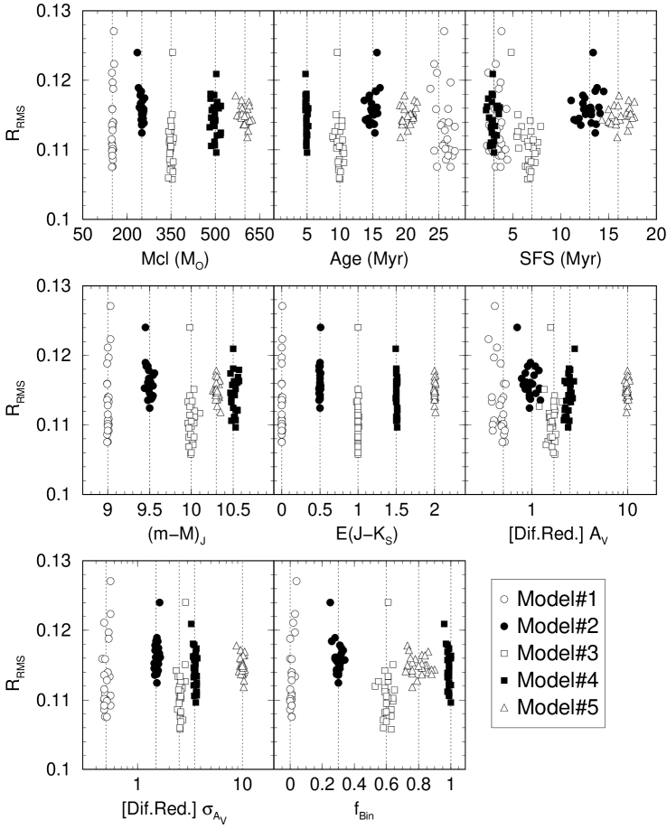
Figure 2: Convergence pattern for the models in Table 1, with the input values shown by the vertical lines. Each symbol represents a single run.

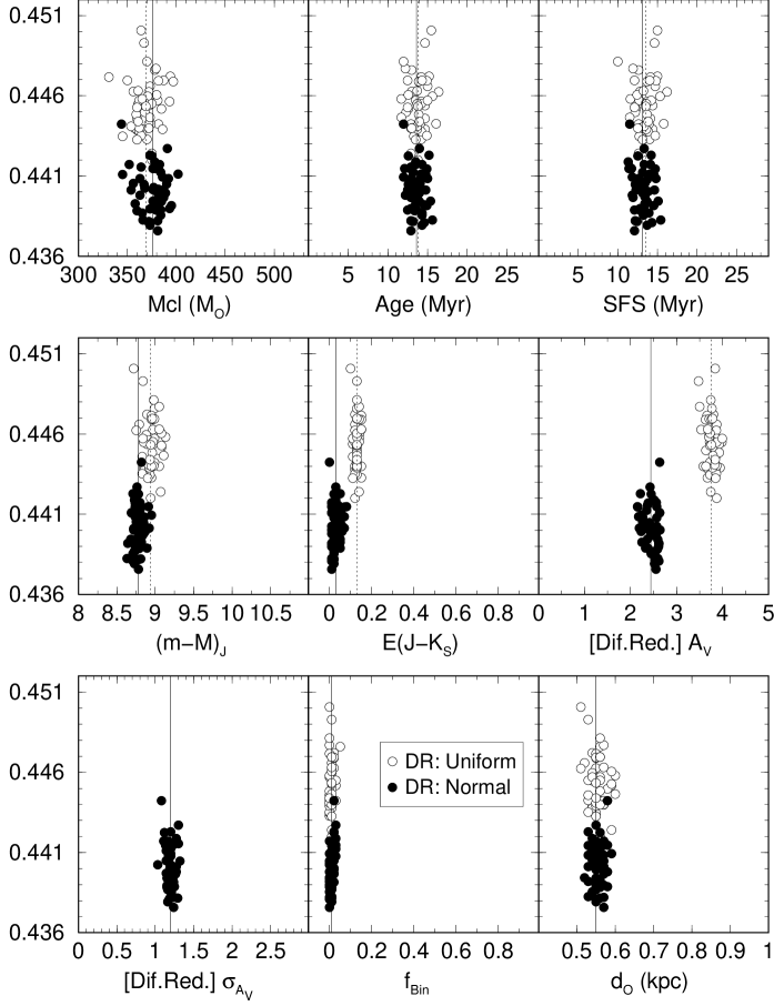
Figure 3: Similar to Fig. 2 for Collinder 197. Results for the uniform (empty symbols) and normal (filled) differential reddening modes are shown. Vertical lines correspond to the mean values for the uniform (dotted) and normal (solid) distributions. The abscissa scales represent the search-ranges used at the beginning of the ASA minimisation process.

Table 1: Recovery of model parameters with $ASA_{min}$

Rank	$R_{rms}$	$M_{clu}$	Age	$\tau_{sfs}$	$(m-M)_{J}$	$E(J-K_{s})$	$\overline{\delta A}_{V}$	$\sigma(\mbox{$\delta A_{V}$})$	$f_{bin}$	$M_{CMD}$
		($\rm M_{\odot}$)	(Myr)	(Myr)	(mag)	(mag)	(mag)	(mag)		($\rm M_{\odot}$)
(1)	(2)	(3)	(4)	(5)	(6)	(7)	(8)	(9)	(10)	(11)
Model#1		150	25	3	9.0	0.0	0.5	0.5	0.0	—
Min	0.1556	149	26.8	3.7	8.99	0.00	0.49	0.51	0.01	133
Max	0.1763	155	25.8	3.8	9.03	0.01	0.41	0.55	0.04	145
Mean	0.1653	$151\pm 2$	$25.9\pm 1.0$	$3.3\pm 0.6$	$9.00\pm 0.01$	$0.01\pm 0.01$	$0.46\pm 0.05$	$0.51\pm 0.03$	$0.01\pm 0.01$	$135\pm 3$
Model#2		250	15	13	9.5	0.5	1.0	1.5	0.3	—
Min	0.1124	250	15.3	13.6	9.50	0.50	0.94	1.53	0.30	153
Max	0.1240	235	15.6	13.4	9.45	0.51	0.70	1.62	0.25	142
Mean	0.1160	$250\pm 6$	$15.0\pm 0.6$	$12.9\pm 0.7$	$9.50\pm 0.03$	$0.50\pm 0.01$	$0.97\pm 0.13$	$1.53\pm 0.05$	$0.30\pm 0.02$	$153\pm 5$
Model#3		350	10	7	10.0	1.0	1.7	2.5	0.6	—
Min	0.1058	354	10.0	6.5	9.99	1.00	1.73	2.54	0.63	200
Max	0.1240	355	9.6	4.8	9.98	1.00	1.57	2.87	0.61	204
Mean	0.1105	$349\pm 5$	$9.9\pm 0.5$	$6.6\pm 0.7$	$10.00\pm 0.03$	$1.00\pm 0.01$	$1.61\pm 0.16$	$2.57\pm 0.12$	$0.60\pm 0.03$	$193\pm 3$
Model#4		500	5	3	10.5	1.5	2.5	3.5	1.0	—
Min	0.1096	503	5.0	3.0	10.53	1.51	2.39	3.59	1.00	278
Max	0.1209	503	4.8	2.9	10.50	1.49	2.81	3.25	0.96	261
Mean	0.1143	$500\pm 11$	$4.9\pm 0.1$	$2.9\pm 0.3$	$10.52\pm 0.03$	$1.50\pm 0.01$	$2.40\pm 0.17$	$3.53\pm 0.11$	$0.99\pm 0.01$	$280\pm 6$
Model#5		600	20	16	10.3	2.0	10.0	10.0	0.8	—
Min	0.1119	609	19.2	15.9	10.35	2.01	9.77	10.28	0.76	154
Max	0.1178	569	19.8	16.1	10.30	2.00	9.97	8.80	0.73	140
Mean	0.1149	$599\pm 14$	$20.3\pm 0.8$	$16.3\pm 1.0$	$10.31\pm 0.02$	$2.00\pm 0.01$	$9.93\pm 0.26$	$9.95\pm 0.40$	$0.80\pm 0.07$	$152\pm 4$

• Cols. (1) and (2): $R_{rms}$ rank and value; Col. (3): actual cluster mass; Col. (4): cluster age; Col. (5): SFS timescale; Col. (6): apparent distance modulus in the $J$ band; Col. (7): foreground reddening; Cols. (8) and (9): mean DR and standard deviation; Col. (10): unresolved binary fraction; Col. (11): cluster mass as measured in the CMD. The average stellar mass of the models is $\overline{m_{*}}\approx 0.6\,\mbox{$\rm M_{\odot}$}$.

As expected, the retrieved parameters close in on the input values as $R_{rms}$ declines, although with somewhat different dispersions around the mean among the parameters. The convergence pattern is clearly tighter for $M_{clu}$, $E(J-K_{s})$, and $(m-M)_{J}$; followed by $\sigma(\mbox{$\delta A_{V}$})$ and $t_{clu}$, with $f_{bin}$, $\tau_{sfs}$, and $\overline{\delta A}_{V}$ at a third level. This is consistent with the mean values and respective standard deviations listed in Table 1. Nevertheless, it is remarkable that $ASA_{min}$ can retrieve the input values even for a CMD with such a high DR amount as that in Model#5. Also, its ability to disentangle DR and binary fraction comes from the fact that, although both effects tend to redden the stellar sequences, binaries brighten them, while DR shifts them towards the opposite direction. It is also interesting the strong sensitivity for very short (e.g. Models#1 and 4) and long (Models#2 and 5) SFSs.

Similarly to Paper I, we also compute the cluster mass that potentially would be measured based on CMD properties ($M_{CMD}$), which is an important piece of information for, e.g., establishing the dynamical state of a cluster. The first step is to find the actual mass of each star occurring in the CMD. However, this may be very difficult to find, especially in the presence of DR, SFS, unresolved binaries, and photometric uncertainties (which decreases the number of stars that remain detectable in a CMD as the distance modulus increases). In practise, what is usually done is: having derived the values of age, distance modulus and foreground reddening, $M_{CMD}$ is computed by finding the probable mass for each star in the CMD by interpolation of the observed colour and magnitude among those of the nearest isochrones. Obviously, the precision of this procedure relies heavily on the amount of DR, photometric noise, binaries, etc. For instance, a heavily differentially reddened cluster of $\mbox{$M_{clu}$}\sim 600\,\mbox{$\rm M_{\odot}$}$, characterised by a moderate binary fraction and distance modulus, would have only $\approx 25\%$ of its actual mass estimated based on CMD properties (e.g., Model#5 in Table 1).

We close this section by concluding that $ASA_{min}$ - the minimisation of residuals between the observed and simulated Hess diagrams by means of ASA - is efficient in retrieving the input parameters of model CMDs that cover a variety of conditions.

5 Probing actual star clusters

Based on the experience gained in Sect. 4.1 with model CMDs, we now move on to investigate actual young clusters with $ASA_{min}$. For this we use Collinder 197 (Bonatto & Bica 2010a) and Pismis 5 (Bonatto & Bica 2009b). Both clusters have been studied in Paper I, which thus will allow us to compare the effect of different assumptions on SFR, DR and binaries, on the derived parameters. They are projected near the Galactic equator ($b\approx 1\degr$) and have CMDs dominated by faint stars. To minimise confusion between intrinsic PMS stars and red dwarfs of the Galactic field, we build field-star decontaminated CMDs by means of the algorithm developed in Bonatto & Bica (2007) and improved in Bonatto & Bica (2010a). As a result, the decontaminated CMD of Collinder 197 has 690 stars (essentially PMS), while Pismis 5 has only 101, which is important for examining the effect of CMDs with different numbers of stars on our analysis. In addition, the colour-colour diagrams of both objects (Collinder 197: Fig. 7 of Bonatto & Bica 2010a; Pismis 5: Fig. 9 of 7Bonatto & Bica 2009b) do not contain detections with abnormally high infrared excesses that might be due to circumstellar material.

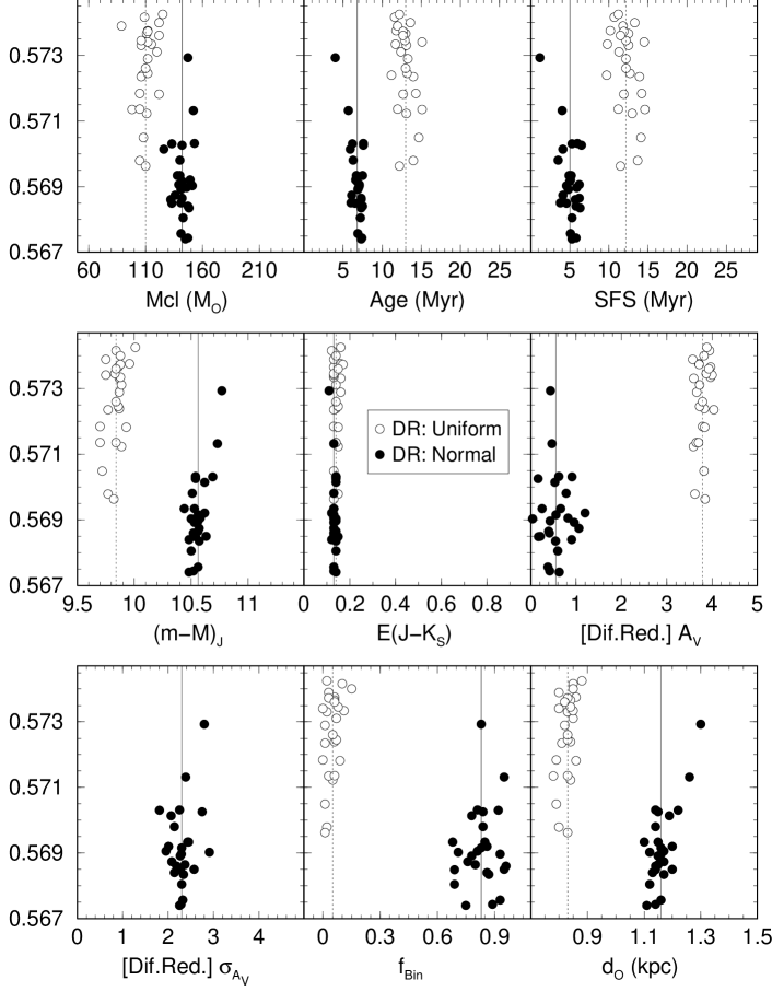
Figure 4: Same as Fig. 3 for Pismis 5.

After several tests with $ASA_{min}$, we settled on $\mbox{$N_{sim}$}=50$ and $\mbox{$N_{run}$}=50$ for Collinder 197 and $\mbox{$N_{sim}$}=500$ and $\mbox{$N_{run}$}=25$ for Pismis 5 as a compromise between convergence pattern and running time. Besides the normal DR distribution, for comparison purposes we also consider the case of a uniform (or flat) distribution. The parameters obtained with $ASA_{min}$ are given in Table 2, and the full set of runs is shown in Figs. 3 and 4. For comparison with other clusters, we also compute the bolometric magnitude and mass to light ratio. We remark that it is significant that convergence patterns reached after several thousand ASA iterations, similar to those of the model CMDs, occur for all parameters of both clusters.

Table 2: Parameters of Collinder 197 and Pismis 5

$R_{rms}$	$M_{clu}$	Age	$\tau_{sfs}$	$(m-M)_{J}$	$E(J-K_{s})$	$\overline{\delta A}_{V}$	$\sigma(\mbox{$\delta A_{V}$})$	$f_{bin}$	$M_{CMD}$	$d_{\odot}$	$10^{3}$ MLR	$M_{BOL}$
	($\rm M_{\odot}$)	(Myr)	(Myr)	(mag)	(mag)	(mag)	(mag)		($\rm M_{\odot}$)	(kpc)	($\mbox{$\rm M_{\odot}$}/L_{\odot}$)	(mag)
(1)	(2)	(3)	(4)	(5)	(6)	(7)	(8)	(9)	(10)	(11)	(12)	(13)
	Collinder 197 - Differential reddening mode: normal
0.4376	381	12.9	12.1	8.78	0.01	2.55	1.24	0.00	211	0.57	4.7	-7.5
0.4442	344	12.0	11.5	8.82	0.00	2.63	1.08	0.02	182	0.58	6.6	-7.0
0.4401	$376\pm 13$	$13.6\pm 0.9$	$13.1\pm 1.0$	$8.78\pm 0.07$	$0.03\pm 0.02$	$2.44\pm 0.15$	$1.20\pm 0.06$	$0.01\pm 0.01$	$208\pm 7$	$0.55\pm 0.02$	$4.2\pm 1.0$	$-7.6\pm 0.2$
$\Delta 1\sigma$	$376^{+230}_{-190}$	$12.9^{+7.2}_{-4.7}$	$12.1^{+0.7}_{-5.3}$	$8.78^{+1.30}_{-0.76}$	$0.01^{+0.17}_{-0.01}$	$2.55^{+1.02}_{-0.96}$	$1.24^{+0.96}_{-0.51}$	$0.00^{+0.39}_{-0.00}$	$211^{+30}_{-56}$	$0.57^{+0.33}_{-0.17}$	$4.7^{+3.3}_{-0.4}$	$-7.5^{-0.1}_{+0.6}$
$\overline{1\sigma}$	$396\pm 96$	$14.3\pm 3.5$	$10.0\pm 1.7$	$8.95\pm 0.47$	$0.01\pm 0.01$	$2.58\pm 0.50$	$1.42\pm 0.40$	$0.17\pm 0.11$	$224\pm 12$	$0.58\pm 0.12$	$3.5\pm 1.9$	$-7.9\pm 0.6$
	Collinder 197 - Differential reddening mode: uniform
0.4420	375	13.8	13.6	8.94	0.12	3.87	—	0.01	225	0.56	5.3	-7.4
0.4501	364	15.5	15.0	8.72	0.10	3.84	—	0.00	224	0.51	4.7	-7.5
0.4453	$369\pm 12$	$13.8\pm 1.1$	$13.5\pm 1.1$	$8.94\pm 0.09$	$0.13\pm 0.01$	$3.76\pm 0.11$	—	$0.01\pm 0.01$	$227\pm 8$	$0.55\pm 0.02$	$4.1\pm 0.8$	$-7.6\pm 0.2$
	Pismis 5 - Differential reddening mode: normal
0.5674	145	7.3	5.3	10.48	0.14	0.63	2.25	0.75	80	1.11	3.1	-6.9
0.5729	147	4.0	1.2	10.77	0.11	0.44	2.80	0.83	100	1.30	1.8	-7.5
0.5692	$142\pm 7$	$6.8\pm 0.8$	$5.0\pm 1.0$	$10.56\pm 0.08$	$0.13\pm 0.01$	$0.56\pm 0.29$	$2.30\pm 0.25$	$0.83\pm 0.08$	$81\pm 4$	$1.16\pm 0.04$	$2.6\pm 0.4$	$-7.1\pm 0.2$
$\Delta 1\sigma$	$145^{+91}_{-83}$	$7.3^{+8.0}_{-3.8}$	$5.3^{+1.8}_{-2.7}$	$10.48^{+0.82}_{-0.72}$	$0.14^{+0.06}_{-0.07}$	$0.63^{+1.25}_{-0.63}$	$2.25^{+1.66}_{-0.85}$	$0.75^{+0.25}_{-0.57}$	$80^{+6}_{-23}$	$1.11^{+0.44}_{-0.25}$	$3.1^{+2.2}_{-0.4}$	$-6.9^{-0.1}_{+0.6}$
$\overline{1\sigma}$	$154\pm 50$	$9.0\pm 3.2$	$5.0\pm 1.3$	$10.52\pm 0.38$	$0.14\pm 0.04$	$0.92\pm 0.54$	$2.62\pm 0.70$	$0.73\pm 0.16$	$82\pm 7$	$1.12\pm 0.20$	$2.7\pm 1.5$	$-7.0\pm 0.6$
	Pismis 5 - Differential reddening mode: uniform
0.5696	110	12.2	11.5	9.82	0.13	3.85	—	0.01	57	0.83	4.5	-6.2
0.5743	125	12.2	11.2	10.01	0.16	3.89	—	0.02	63	0.88	4.5	-6.4
0.5726	$110\pm 8$	$13.0\pm 1.1$	$12.2\pm 1.2$	$9.84\pm 0.08$	$0.14\pm 0.01$	$3.79\pm 0.13$	—	$0.05\pm 0.04$	$57\pm 4$	$0.83\pm 0.03$	$4.4\pm 0.9$	$-6.3\pm 0.2$

• Col. (1): minimum, maximum and mean $R_{rms}$ values; Col. (2): actual cluster mass; Col. (3): cluster age; Col. (4): SFS; Col. (5): apparent distance modulus in the $J$ band; Col. (6): foreground reddening; Cols. (7) and (8): differential reddening; Col. (9): unresolved binary fraction; Col. (10): cluster mass as measured in the CMD; Col. (11): distance from the Sun; Col. (12): bolometric mass to light ratio; Col. (13): bolometric magnitude. $\Delta 1\sigma$: parameters occurring at the boundaries of the $1\sigma$ domain. $\overline{1\sigma}$: weighted average of values occurring within the $1\sigma$ domain.

In both cases, the $R_{rms}$ corresponding to the normal DR distribution tends to be lower than those of the uniform distribution. Also, reflecting the larger number of CMD stars, the $R_{rms}$ values of Collinder 197 are significantly lower than those of Pismis 5.

Before moving on to interpreting the results, it is important to remind that each $R_{rms}$ value and corresponding optimum parameters result from several thousand iterations, as ASA searches the $R_{rms}$ hyper-surface for the absolute minimum of Eq. 1. At each iteration, $N_{sim}$ twin clusters (i.e., consisting of exactly the same set of parameters) are built and incorporated into the simulated Hess diagram. Thus, the occurrence of a tight convergence pattern for the absolute minimum parameters over a series of independent runs shows a self consistency of the method and cannot be taken as fortuitous or model dependent. Instead, it would be strongly indicative that the optimum parameters produced by $ASA_{min}$ are indeed representative of those of the cluster being studied. On the other hand, we remark that this argument applies only to the absolute minimum of each $ASA_{min}$ run, since the $R_{rms}$ topology around this feature is not taken into account. In this sense, the quoted errors should be taken as internal, probably not reflecting the realistic parameter uncertainties. Indeed, as we show in Sect. 5.2, in some cases the drop towards the absolute minimum is somewhat gentle, which means that there can be a significant dispersion (different values at similar $R_{rms}$ levels) around the absolute minima. Although the depression shape departs from gaussianity, we estimate the approximate extension of the $1\sigma$ domain and compute the weighted mean and dispersion for the parameters occurring inside it (again using the individual $R_{rms}$ as weight). The results - restricted to the uniform DR - are given in the additional entry labelled as $\overline{1\sigma}$ in Table 2. Compared to the previous statistics, the uncertainties now are more realistic and consistent both with the $R_{rms}$ topology and the assumptions incorporated into the simulations. For completeness, we also provide in Table 2 the parameter values that occur at the boundaries of the $1\sigma$ domain (labelled as $\Delta 1\sigma$). In general, they imply considerably larger errors than before. However, given the underlying assumption of residual minimisation and respective $R_{rms}$ value of different parameter sets, we believe that the weighted-mean values ($\overline{1\sigma}$) are more representative for the clusters dealt with in this work. In addition, the mean values are essentially unchanged, except for a somewhat higher binary fraction for Collinder 197.

Collinder 197:

The values of cluster mass, age, SFS, binary fraction, and distance from the Sun are essentially insensitive to the DR mode. They consistently indicate a cluster of $\mbox{$M_{clu}$}\approx 400\,\mbox{$\rm M_{\odot}$}$, $\mbox{$t_{clu}$}\approx 14$ Myr, $\mbox{$\tau_{sfs}$}\approx 10$ Myr, with a relatively low binary fraction of $\mbox{$f_{bin}$}\la 0.2$, located at $\approx 0.6$ kpc from the Sun. However, assuming that representativeness increases for lower $R_{rms}$ values, DR in this cluster would follow a normal distribution characterised by $\mbox{$\overline{\delta A}_{V}$}\approx 2.6$ and $\mbox{$\sigma(\mbox{$\delta A_{V}$})$}\approx 1.4$. The differences that occur in distance modulus and foreground reddening can be accounted for by the single, fixed value of $\delta A_{V}$ of the uniform DR distribution, which requires higher values of $(m-M)_{J}$ and $E(J-K_{s})$ than the normal mode to account for the observed colour spread of the stellar sequences. The foreground reddening is very low, corresponding to $\mbox{$A_{V}$}\approx 0.1$.

Pismis 5:

Compared to Collinder 197, here the DR modes result in significant differences for most of the cluster parameters, except for the foreground reddening. Also, as expected from the lower number of stars, the convergence patterns are in general looser than for Collinder 197. Perhaps the most contrasting result lies in the binary fraction that reaches $\mbox{$f_{bin}$}\approx 0.7$. Lacking one degree of freedom, the uniform DR mode tries to describe the CMD spread by assuming a large value of $\overline{\delta A}_{V}$ with essentially no binaries. In contrast, the normal mode requires a lower $\overline{\delta A}_{V}$ with a high dispersion $\sigma(\mbox{$\delta A_{V}$})$, which yields a high binary fraction. Combined, the low $\overline{\delta A}_{V}$ and high $f_{bin}$ of the normal mode put Pismis 5 at a distance $\sim 40\%$ larger than that implied by the uniform mode. The foreground reddening, $\mbox{$A_{V}$}\approx 0.9$, is higher than that of Collinder 197.

Interestingly, because of the additional free parameter, the normal DR distribution produces a cluster age significantly younger than that implied by the uniform distribution, especially for Pismis 5. Also, in both cases the SFS is equivalent to $\sim 60\%$ of the cluster age.

Comparing the values obtained by $ASA_{min}$ with those in Paper I, we see that now the ages tend to be somewhat older and the distances shorter, with a reasonable agreement among the other parameters. A similar conclusion applies to the scarce works on both objects. Previous estimates for Collinder 197 are: age$\sim 5\pm 4$ Myr, $\mbox{$d_{\odot}$}\sim 1.1\pm 0.2$ kpc, and mass $100-500\,\mbox{$\rm M_{\odot}$}$ (Bonatto & Bica 2010a, and references therein). For Pismis 5, they are: age $5-15$ Myr and $\mbox{$d_{\odot}$}\sim 1.0\pm 0.2$ kpc (Bonatto & Bica 2009b, and references therein). In paper I we had assumed a constant SFR, uniform DR and a fixed binary fraction. Despite the latter two effects, the main source of differences is the SFR. In a constant SFR, stars of any age have the same probability of being formed, and young stars are significantly brighter than their older counterparts. Thus, when trying to match the same observed CMD, a simulation that contains an enhanced population of young stars (constant SFR) would require higher values of distance modulus than another based on a decaying SFR. At the same time, the constant SFR simulation would also imply a younger age.

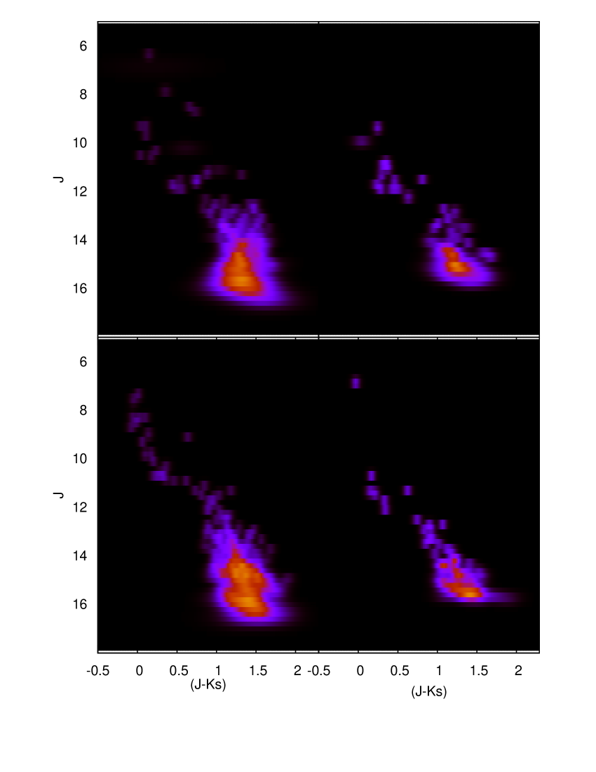
Figure 5: Observed (top panels) and simulated (bottom) Hess diagrams of Collinder 197 (left) and Pismis 5 (right). Lighter grey shades indicate higher densities of stars. The simulated diagrams have been built with the mean parameters and the normal DR mode (Table 2).

The representativeness reached by the minimisation process described above for Collinder 197 and Pismis 5 can be visually appreciated by comparing the observed and simulated Hess diagrams (Fig. 5). The latter have been constructed with the mean parameters and assuming the normally-distributed DR (Table 2). Although the occurrence of some discreteness in both Hess diagrams, which is a natural consequence of the relatively low-mass nature of the clusters, especially for Pismis 5, observation and simulation show a reasonable correspondence in both clusters.

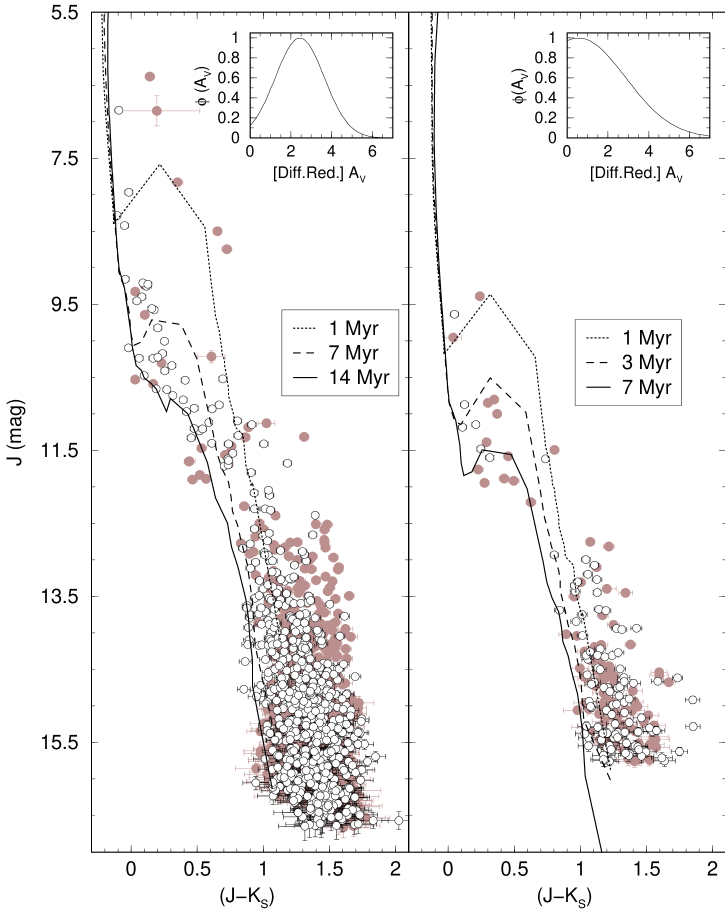
Figure 6: Field-star decontaminated CMDs (light-shaded circles) of Collinder 197 (left) and Pismis 5 (right) compared to a single realisation taken from the respective simulations (empty circles). The extraction radii are 10′ (Collinder 197) and 6′ (Pismis 5). Isochrones representing the star-formation history have been set according to the mean parameters (Table 2). Insets show the DR distribution.

Finally, in Fig. 6 we compare a single CMD realisation randomly selected among the $N_{sim}$ simulated clusters - but having exactly the same number of stars - with the observed CMDs. The DR distributions (Collinder 197 has higher $\overline{\delta A}_{V}$ and lower $\sigma(\mbox{$\delta A_{V}$})$ than Pismis 5) are also shown. For illustrative purposes, Fig. 6 also shows the isochrones that represent the full star-formation history of both clusters. They have been set with the mean values of distance modulus and foreground reddening in Table 2. Note that the optimum simulation and respective isochrone solution end up naturally respecting the blue border of the observed stellar sequences as a (not-imposed) boundary condition. Also, the fading and reddening effect of DR on the stars is clearly seen when one compares the youngest (and reddest) isochrone with the redwards spread of the PMS stellar sequences. This also shows that, if DR is not properly taken into account, fitting isochrones to a CMD would require somewhat younger ages coupled to higher values of distance modulus and foreground reddening, especially to account for the faint and red PMS stars together with the blue border.

Again, given that both are low-mass, young clusters, some morphological differences should be statistically expected, especially in the MS. Nevertheless, simulated and observed CMDs are similar in both cases.

5.1 The low-mass stochasticity

An interesting issue that can be investigated with $ASA_{min}$ is the natural stochasticity associated with low-mass clusters. In other words, how the number of simulated clusters ($N_{sim}$) affect the convergence pattern of the retrieved parameters. Obviously, $N_{sim}$ is expected to play an important role especially on a poorly-populated ($\mbox{$M_{clu}$}<150\,\mbox{$\rm M_{\odot}$}$) and young ($\mbox{$t_{clu}$}\sim 7$ Myr) cluster such as Pismis 5, in which the stochasticity tends to be critical.

For a low-mass cluster consisting essentially of PMS stars, the stochasticity issue can be summarised as follows. Statistically, a random simulation of this cluster (same age, mass, etc) may contain a massive, bright star that is not present in the actual cluster. Consequently, because of the mass constraint, the CMD of this particular simulation would also lack a large fraction of the low-mass content. Thus, despite having been built with exactly the same parameters as the cluster, the $R_{rms}$ residuals of this simulation would be large, with a low representativeness. Given the extremely large number of parameter combinations, the probability of finding a single simulation with a Hess diagram matching that of the cluster is vanishingly low. On the other hand, when many simulations with exactly the same parameters are considered, the individual Hess diagrams would certainly present different representativeness. Thus, the average Hess diagram over many simulations is expected to present a higher similarity (i.e., low $R_{rms}$) with that of a cluster’s than what would be obtained with a single, random simulation. It is in this context that averaging out several simulations of such twin clusters becomes an effective way of minimising stochasticity.

Such effect is illustrated in Fig. 7, in which we show the retrieved parameters for Pismis 5 after running $ASA_{min}$ with $\mbox{$N_{sim}$}=10,\leavevmode\nobreak\ 100$ and $500$, always assuming the same initial conditions. Clearly, the convergence pattern, which is very loose for $\mbox{$N_{sim}$}=10$, becomes tighter as $N_{sim}$ increases. Despite the significant scatter associated mainly with $\mbox{$N_{sim}$}=10$, it is interesting to note that at the lowest $R_{rms}$ values, the parameters of $\mbox{$N_{sim}$}=10$ and $100$ converge to those of $\mbox{$N_{sim}$}=500$. Besides, the differences between the $\mbox{$N_{sim}$}=100$ and $\mbox{$N_{sim}$}=500$ runs are significantly smaller than those between $\mbox{$N_{sim}$}=10$ and $\mbox{$N_{sim}$}=100$.

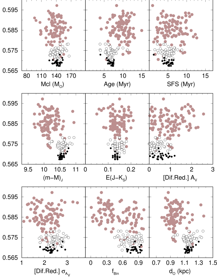
Figure 7: Increasing the number of twin simulations ($N_{sim}$) improves the convergence pattern for a poorly-populated cluster such as Pismis 5. Simulations built assuming the normal DR mode. The number of simulations used in the runs are $\mbox{$N_{sim}$}=10$ (light-shaded circles), $\mbox{$N_{sim}$}=100$ (empty), and $\mbox{$N_{sim}$}=500$ (filled).

Note, however, that some scatter is still present for SFS, mean DR and dispersion, and binary fraction, even when $\mbox{$N_{sim}$}=500$. Ideally, a very large $N_{sim}$ should be used to reach a very tight convergence pattern for a low-mass cluster. In practice, however, this may lead to exceedingly long runtimes. In this sense, our recipe of using a moderate $N_{sim}$ combined to a series of runs may be taken as a compromise between runtime and robustness.

5.2 $ASA_{min}$ and the $R_{rms}$ topology

Having found the best-fit parameters, we now use them to examine the topology of the $R_{rms}$ hyper-surface, something we address by means of selected two-dimensional projections (Fig. 8). For statistical significance, the maps were produced with $\mbox{$N_{sim}$}=100$ and $500$ and the absolute minimum $R_{rms}$ parameters, respectively for Collinder 197 and Pismis 5. The presence of a minimum is clear, but with convergence patterns varying significantly among the parameters, being tight for most but somewhat loose especially for the binary fraction.

Interestingly, the projections now are significantly smoother and with less features than the equivalent ones shown in Fig. 5 of Paper I. Possible reasons for such a contrast are that in Paper I the $R_{rms}$ hyper-surface (i) was built using some fixed parameters (binary fraction and SFS) and restrictive conditions (flat SFR and uniform DR distribution), (ii) the free parameters were allowed to vary within bins of fixed size (and not continuously as in the present approach) and within restricted ranges, and (iii) we used a different statistics for finding solutions. Apparently, the additional free parameters and less-restrictive conditions have raised the degeneracy of solutions found in Paper I.

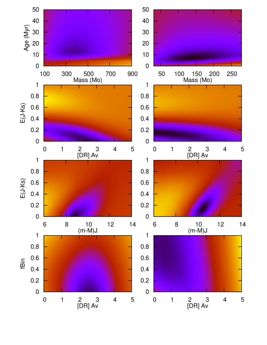
Figure 8: Selected two-dimensional $R_{rms}$ projections for Collinder 197 (left) and Pismis 5 (right). Darker colours indicate lower $R_{rms}$. Convergence patterns vary significantly among different parameters.

In any case, what is really important for our approach is the existence of at least one conspicuous minimum, and our expectation (Sect. 4) is that ASA is efficient in finding its way towards the absolute minimum. In addition, a single minimum also serves to strengthen the unicity of the solutions. Thus, given the relevance of this assumption to the results discussed above, we summarise it in Fig. 9 with one-dimensional projections of the $R_{rms}$ hyper-surface for selected parameters of both clusters. For instance, we take from Table 2 the minimum values (obtained with the normal DR mode) for all the parameters except cluster mass, which is allowed to vary within a wide range (in this case, $0.5\leq\mbox{$M_{clu}$}(\mbox{$\rm M_{\odot}$})\leq 250$). Then, we compute $R_{rms}$ for masses within the adopted range, but keeping the remaining parameters fixed. For a deeper perspective on the effect of parameter variation on the $R_{rms}$ shape, this step is repeated with the fixed parameters changed to 10% higher and lower than the optimum values. The same procedure is applied to the age, mean DR and binary fraction.

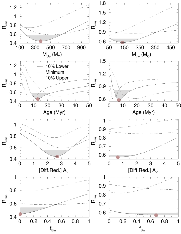
Figure 9: Selected one-dimensional projections of $R_{rms}$ computed with $\mbox{$N_{sim}$}=500$ for Collinder 197 (left) and $\mbox{$N_{sim}$}=1500$ for Pismis 5 (right). Besides the values computed for the absolute minimum parameters (solid line), we also show the $R_{rms}$ projections using values 10% lower (dotted) and higher (dashed) than the minimum. The absolute minimum is shown by the shaded circle, and the approximate $1\sigma$ domain is shown by the grey region.

Consistently with the $R_{rms}$ maps (Fig. 8), the selected $R_{rms}$ projections present a single minimum with a degree of definition (depth and width) that varies significantly among the adopted thresholds. When comparing different parameters, the minima tend to be quite narrow and deep for the age, somewhat wide and shallow for the binary fraction, and intermediate for the remaining parameters.

The general conclusions emerging from the above discussion are: (i) the $R_{rms}$ hyper-surface contains at least one minimum within the adopted search range, (ii) the morphological features of the minimum vary according to each parameter, and most importantly, (iii) $ASA_{min}$ finds its way through the $R_{rms}$ topology towards the absolute minimum.

6 Summary and conclusions

A new approach ($ASA_{min}$), designed to obtain a set of important parameters of young star clusters at a statistically significant confidence level, is presented in this paper. In short, it is essentially based on photometric properties and involves building realistic simulations of the Hess diagram of an actual star cluster, from which the residuals ($R_{rms}$) with respect to the observed Hess diagram are computed. Besides cluster mass, age, foreground reddening and distance modulus, the simulations include the SFS, (alternative modes of) DR and the binary fraction as free parameters. The CMD spread due to photometric uncertainties is explicitly taken into account. Important features of the simulations are a linearly decreasing SFR and a normally distributed DR.

To find the absolute minimum of the $R_{rms}$ hyper-surface we use the global optimisation method known as adaptive simulated annealing (ASA), which is rather efficient and capable of escaping from local depressions. Given the highly-statistical nature of the simulations (and the cluster stochasticity), we show that an acceptable parameter-retrieval rate is achieved by combining a moderate number of simulated clusters with a series of independent ASA runs, while realistic errors in the derived parameters are obtained by exploring properties of the depression shape. Tests with model clusters built with a broad range of parameters show that the distribution of retrieved values (corresponding to the absolute $R_{rms}$ minimum) usually follows a convergence pattern that is tighter as $R_{rms}$ declines, with the same occurring with actual clusters. We also find that the parameter retrieval presents a high sensitivity for cluster mass, distance modulus and foreground reddening, but dropping somewhat for the remaining parameters.

We remark that the particular results discussed in this work may be somewhat model dependent, in the sense that they are based on the 2MASS near-infrared photometry coupled to the Padova and Siess MS and PMS isochrone sets. Other isochrones with somewhat different mass to light ratios for individual stars may possibly affect the star cluster parameters when retrieved by $ASA_{min}$, especially the age, mass and distance. In any case, $ASA_{min}$ can be easily adapted to any photometric system (and isochrone set), provided the respective MS and PMS isochrones and the relation of photometric errors with magnitude are available. However, by allowing a deeper view through the dust, the near-infrared seems to be the best window to disentangle the effects of DR, binaries and SFS.

In summary, we show in this work that our semi-analytical and comprehensive approach is capable of uncovering a series of parameters of young clusters, even when photometry is the only available information. Among these, the cluster age, star-formation spread, mass and binary fraction are important for establishing the dynamical state of a cluster, or derive a more precise SFR in the Galaxy.

References

- Bate (2011) Bate M.R. 2011, in Computational Star Formation, Proceedings of the International Astronomical Union, IAU Symposium, Volume 270, p. 133-140, editors: J. Alves, B.G. Elmegreen, J. M. Girart & V. Trimble
- Belloche et al. (2011) Belloche A., Schuller F., Parise B., André Ph., Hatchell J., Jørgensen J.K., Bontemps S., Wei A. et al. 2011, A&A, 527, 145
- Bica, Bonatto & Dutra (2008) Bica E., Bonatto C. & Dutra C.M. 2008, A&A, 489, 1129
- Bonatto, Santos Jr. & Bica (2006) Bonatto C., Santos Jr. J.F.C. & Bica E. 2006, A&A, 445, 567
- Bonatto et al. (2006) Bonatto C., Bica E., Ortolani S. & Barbuy B. 2006, A&A, 453, 121
- Bonatto & Bica (2007) Bonatto C. & Bica E. 2007, MNRAS, 377, 1301
- Bonatto & Bica (2009a) Bonatto C. & Bica E. 2009a, MNRAS, 394, 2127
- Bonatto & Bica (2009b) Bonatto C. & Bica E. 2009b, MNRAS, 397, 1915
- Bonatto & Bica (2010a) Bonatto C. & Bica E. 2010a, A&A, 516, 81
- Bonatto & Bica (2010b) Bonatto C. & Bica E. 2010b, A&A, 521A, 74
- Bonatto & Bica (2011) Bonatto C. & Bica E. 2011, MNRAS, 415, 2827
- Bonatto, Bica & Lima (2011) Bonatto C., Bica E. & Lima E.F. 2012, MNRAS, 420, 352 (Paper I)
- Cardelli, Clayton & Mathis (1989) Cardelli J.A., Clayton G.C. & Mathis, J.S. 1989, ApJ, 345, 245
- Dutra, Santiago & Bica (2002) Dutra C.M., Santiago B.X. & Bica E. 2002, A&A, 383, 219
- Girardi et al. (2002) Girardi L., Bertelli G., Bressan A., Chiosi C., Groenewegen M.A.T., Marigo P., Salasnich B. & Weiss A. 2002, A&A, 391, 195
- Goffe, Ferrier & Rogers (1994) Goffe W.L., Ferrier G.D. & Rogers J. 1994, Journal of Econometrics, 60, 65
- Goodwin (2009) Goodwin S.P. 2009, Ap&SS, 324, 259
- Goodwin & Bastian (2006) Goodwin S.P. & Bastian N. 2006, MNRAS, 373, 752
- Hess (1924) Hess R. 1924, in Die Verteilungsfunktion der absol. Helligkeiten etc. Probleme der Astronomie. Festschrift fur Hugo v. Seeliger. (Berlin:Springer), 265
- Hillenbrand, Bauermeister & White (2008) Hillenbrand L.A., Bauermeister A. & White R.J. 2008, in 14th Cambridge Workshop on Cool Stars, Stellar Systems, and the Sun, ASP Conference Series, Vol. 384, proceedings of the conference held 5-10 November, 2006, at the Spitzer Science Center and Michelson Science Center, Pasadena, California, USA. Edited by Gerard van Belle., p.200
- Kenyon & Hartmann (1995) Kenyon S.J. & Hartmann L. 1995, ApJS, 101,117
- Kroupa (2001) Kroupa P. 2001, MNRAS, 322, 231
- Lada & Lada (2003) Lada C.J. & Lada E.A. 2003, ARA&A, 41, 57
- Lamers & Gieles (2006) Lamers H.J.G.L.M. & Gieles M. 2006, A&A, 455, L17
- Lamers, Baumgardt & Gieles (2010) Lamers H.J.G.L.M., Baumgardt H. & Gieles M. 2010, MNRAS, 409, 305
- Metropolis et al. (1953) Metropolis N., Rosenbluth A., Rosenbluth M., Teller A. & Teller, E. 1953, Journal of Chemical Physics, 21, 1087
- Naylor & Jeffries (2006) Naylor T. & Jeffries R.D. 2006, MNRAS, 373, 1251
- da Rio, Gouliermis & Gennaro (2010) da Rio N., Gouliermis D.A. & Gennaro M. 2010, ApJ, 723, 166
- Siess, Dufour & Forestini (2000) Siess L., Dufour E. & Forestini M. 2000, A&A, 358, 593
- Skrutskie et al. (2006) Skrutskie M.F., Cutri R., Stiening R., Weinberg M.D., Schneider S.E., Carpenter J.M., Beichman C., Capps R. et al. 2006, AJ, 131, 1163
- Stauffer et al. (1997) Stauffer J.R., Hartmann L.W., Prosser C.F., Randich S., Balachandran S., Patten B.M., Simon T. & Giampapa M. 1997, ApJ, 479, 776
- Stead & Hoare (2011) Stead J. & Hoare M. 2011, MNRAS, 418, 2219
- Tutukov (1978) Tutukov A.V. 1978, A&A, 70, 57
- Weidner, Kroupa & Maschberger (2009) Weidner C., Kroupa P. & Maschberger T. 2009, MNRAS, 393, 663