Rank/Norm Regularization with Closed-Form Solutions:
Application to Subspace Clustering

Abstract

When data is sampled from an unknown subspace, principal component analysis (PCA) provides an effective way to estimate the subspace and hence reduce the dimension of the data. At the heart of PCA is the Eckart-Young-Mirsky theorem, which characterizes the best rank $k$ approximation of a matrix. In this paper, we prove a generalization of the Eckart-Young-Mirsky theorem under all unitarily invariant norms. Using this result, we obtain closed-form solutions for a set of rank/norm regularized problems, and derive closed-form solutions for a general class of subspace clustering problems (where data is modelled by unions of unknown subspaces). From these results we obtain new theoretical insights and promising experimental results.

1 Introduction

Real world data, while typically being very high dimensional, often only depends intrinsically on a few parameters (Seung and Lee,, 2000). It is therefore desirable to identify the low dimensional subspace (manifold) from which the data is sampled. Principal component analysis (PCA) (Jolliffe,, 2002) is a classical, yet still popular, method to perform such dimensionality reduction. If the data is sampled from a single subspace, PCA is provably correct in identifying the underlying subspace. Algorithmically, the success of PCA depends critically on the Eckart-Young-Mirsky theorem (Eckart and Young,, 1936; Mirsky,, 1960), which characterizes, in closed-form, the optimal rank $k$ approximation of an arbitrary matrix, under all unitarily invariant norms.

However, in practice it is more likely that data is sampled, not from a single subspace, but from a union of subspaces (Vidal,, 2011). Had we known the membership of the data, the task would be easy: we would just apply PCA to each subset. Unfortunately, one does not normally have such useful membership information a priori. The subspace clustering problem, therefore, is to find the dimension and basis for each subspace while segmenting/clustering the points accordingly. Of course, the primary difficulty is that estimation and segmentation must occur simultaneously, even though either task can be easily accomplished given the result of the other. For applications of subspace clustering, we refer the reader to the recent survey (Vidal,, 2011).

Many algorithms have been proposed for subspace clustering, including factorization methods (Costeira and Kanade,, 1998; Zelnik-Manor and Irani,, 2006), generalized principal component analysis (GPCA) (Vidal et al.,, 2005), and agglomerative lossy compression (Ma et al.,, 2007), as well as the more recent sparse subspace clustering (SSC) (Elhamifar and Vidal,, 2009) and low rank representation (LRR) (Liu et al., 2010b, ), to name a few. GPCA is provably correct while SSC and LRR are provably correct under the independent subspace assumption. However, most current algorithms are computationally extensive, requiring sophisticated numerical optimization routines.

To develop simple algorithms for subspace clustering, we start by generalizing the Eckart-Young-Mirsky theorem (Eckart and Young,, 1936; Mirsky,, 1960), since it is the foundation for PCA in the single subspace scenario. In Section 2, we prove a generalized version of the Eckart-Young-Mirsky theorem under all unitarily invariant norms. The motivation for considering all unitarily invariant norms is not solely for mathematical completeness, it also arises from the increasing popularity of the trace norm, a special unitarily invariant norm. Using similar techniques, we are also able to provide closed-form solutions for some interesting rank/norm regularized problems. The subsequent connections to known results are discussed.

In Section 3, we then apply the results established in Section 2 to the subspace clustering problem. Previous work by Liu et al., 2010b has proven that minimizing the trace norm of the reconstruction matrix yields a suitable block sparse matrix that will reveal the membership of the points in the ideal noiseless setting. We prove that this is not only true for the trace norm, but for essentially all unitarily invariant norms and the rank function. Progressing to the noisy case, we propose to choose suitable combinations of unitarily invariant norms and the rank function in the objective, as it will lead to very simple algorithms that remain provably correct if the data is clean and obeys the independent subspace assumption. Interestingly, the algorithms we propose are intimately related to classic factorization methods (Costeira and Kanade,, 1998; Zelnik-Manor and Irani,, 2006). Experiments on both synthetic data and the hopkins155 motion segmentation dataset (Tron and Vidal,, 2007) demonstrate that the simple algorithms we devise perform comparably with the state-of-the-art algorithms in subspace clustering, while being computationally much cheaper.

Notations: We use $\mathbb{M}^{m\times n}$ to denote $m\times n$ matrices, although generally we will not be very specific about the sizes. $\|\cdot\|_{{\scriptscriptstyle\mathtt{F}}},\|\cdot\|_{{\scriptscriptstyle\mathtt{sp}}},\|\cdot\|_{{\scriptscriptstyle\mathtt{tr}}}$ denote the Frobenius norm, spectral norm, and trace norm, respectively. For any matrix $A$, $A^{*}$ denotes its conjugate transpose, $A^{\dagger}$ its pseudo-inverse, and $A_{(k)}$ its truncation, where the singular vectors are kept but all singular values are zeroed out except the $k$ largest.

In this extended version of the paper, all proofs for the main results stated in the next section are provided in the appendix.

2 Main Results

First we require some definitions. A matrix norm $\|\cdot\|$ is called unitarily invariant if $\|UAV\|=\|A\|$ for all $A\in\mathbb{M}^{m\times n}$ and all unitary matrices $U\in\mathbb{M}^{m\times m}$, $V\in\mathbb{M}^{n\times n}$. We use $\|\cdot\|_{{\scriptscriptstyle\mathtt{UI}}}$ to denote unitarily invariant norms while $\|\cdot\|_{{\scriptscriptstyle\mathtt{AUI}}}$ means (simultaneously) all unitarily invariant norms.

Perhaps the most important examples for unitarily invariant norms are:

$$\|A\|_{(k,p)}:=\Big{(}\sum_{i=1}^{k}\sigma_{i}^{p}\Big{)}^{1/p},$$ (1)

where $p\geq 1$, $k$ is any natural number smaller than $\mathrm{rank}(A)$, and $\sigma_{i}$ is the $i$-th largest singular value of $A$. For $k=\mathrm{rank}(A)$, (1) is known as Schatten’s $p$-norm; while for $p=1$, it is called Ky Fan’s norm. Some special cases include the spectral norm ($p=\infty$), the trace norm ($p=1$, $k=\mathrm{rank}(A)$), and the Frobenius norm ($p=2$, $k=\mathrm{rank}(A)$). Note that all three norms belong to the Schatten’s family while only the first two norms are in the Ky Fan family.

The following theorem is well-known:

Theorem 1

Fix $\mathbb{N}\ni k\leq\mathrm{rank}(A)$, then $A_{(k)}$ is a minimum Frobenius norm solution of

$$\min_{X:~{}\mathrm{rank}{X}\leq k}\|A-X\|_{{\scriptscriptstyle\mathtt{AUI}}}.$$ (2)

The solution is unique iff the $k$-th and $(k+1)$-th largest singular values of $A$ differ.

Theorem 1 was first proved by Eckart and Young, (1936) under the Frobenius norm; and then generalized to all unitarily invariant norms by Mirsky, (1960). The remarkable aspect of Theorem 1 is that although the rank constraint is highly nonlinear and nonconvex, one is still able to solve (2) globally and efficiently by singular value decomposition (SVD). Moreover, the optimal solution under the Frobenius norm remains optimal under all unitarily invariant norms.

The Frobenius norm seems to be very different from other unitarily invariant norms, since it is induced by an inner product and block decomposable. Therefore it is usually much easier to work with the Frobenius norm, and much stronger results can be obtained in this case. For instance, we have the following generalization of Theorem 1 (though less well-known).

For an arbitrary matrix $B$ with rank $r$, we denote its thin SVD as: $B=U_{B}\Sigma_{B}V_{B}^{*}$. Define two projections $P_{B,\mathcal{L}}:=U_{B}U_{B}^{*}$ and $P_{B,\mathcal{R}}:=V_{B}V_{B}^{*}$. Let $U_{B}^{\perp}$ and $V_{B}^{\perp}$ be the orthogonal complement of $U_{B}$ and $V_{B}$, respectively.

Theorem 2

Fix $\mathbb{N}\ni k\leq\mathrm{rank}(P_{B,\mathcal{L}}AP_{C,\mathcal{R}})$, then $B^{{\dagger}}(P_{B,\mathcal{L}}AP_{C,\mathcal{R}})_{(k)}C^{{\dagger}}$ is a minimum Frobenius norm solution of

$$\min_{X:~{}\mathrm{rank}{X}\leq k}\|A-BXC\|_{{\scriptscriptstyle\mathtt{F}}}.$$ (3)

The solution is unique iff the $k$-th and $(k+1)$-th largest singular values of $P_{B,\mathcal{L}}AP_{C,\mathcal{R}}$ differ.

Theorem 2 was first proved by Sondermann, (1986), but largely remained unnoticed. It was rediscovered recently by Friedland and Torokhti, (2007). One may prove Theorem 2 fairly easily, for instance, by adapting our proof for Theorem 3 below (plus the observation that the Frobenius norm is block decomposable).

One natural question is whether we can replace the Frobenius norm in Theorem 2 with other unitarily invariant norms, as in Theorem 1. Unfortunately, Example 2 below shows that it is impossible in general. However, by putting assumptions on $A,B$ and $C$, we are able to generalize Theorem 2 in meaningful ways.

Simultaneous Block Assumption (SB): Assume $(U_{B}^{\perp})^{*}AV_{C}=0$ and $U_{B}^{*}AV_{C}^{\perp}=0$.

Theorem 3

Fix $\mathbb{N}\ni k\leq\mathrm{rank}(P_{B,\mathcal{L}}AP_{C,\mathcal{R}})$. Under the SB assumption, $B^{{\dagger}}(P_{B,\mathcal{L}}AP_{C,\mathcal{R}})_{(k)}C^{{\dagger}}$ is a minimum Frobenius norm solution of

$$\min_{X:~{}\mathrm{rank}{X}\leq k}\|A-BXC\|_{{\scriptscriptstyle\mathtt{AUI}}}.$$ (4)

The solution is unique iff the $k$-th and $(k+1)$-th largest singular values of $P_{B,\mathcal{L}}AP_{C,\mathcal{R}}$ differ.

The next proposition plays a key role in the proof of Theorem 3, and may be of some independent interest.

Proposition 1

If it exists, any minimizer of

$$\min_{X\in\mathcal{X}}\|X\|_{{\scriptscriptstyle\mathtt{AUI}}}$$ (5)

remains optimal for

$$\min_{X\in\mathcal{X}}\left\|\begin{pmatrix}X&0\\ 0&B\end{pmatrix}\right\|_{{\scriptscriptstyle\mathtt{AUI}}}$$

for any constant matrix $B$.

Remark 1

It is our incapability of extending Proposition 1 to full block matrices, $\begin{pmatrix}X&C\\ D&B\end{pmatrix}$, that prevents us from fully generalizing Theorem 2.

One interesting case where the SB assumption is trivially satisfied can be summarized as:

Corollary 1

Fix $\mathbb{N}\ni k\leq\mathrm{rank}(A)$, then $B^{{\dagger}}(BAC)_{(k)}C^{{\dagger}}$ is a minimum Frobenius norm solution of

$$\min_{X:~{}\mathrm{rank}{X}\leq k}\|BAC-BXC\|_{{\scriptscriptstyle\mathtt{AUI}}}.$$ (6)

The solution is unique iff the $k$-th and $(k+1)$-th largest singular values of $BAC$ differ.

Setting $B$ and $C$ to identities, we recover Theorem 1. Note that a special case of this corollary (where $B$ is identity and $C$ is a projection) has been previously established in (Piotrowski and Yamada,, 2008; Piotrowski et al.,, 2009) in the context of reduced-rank estimators. However, our corollary is stronger and obtained by a much simpler proof. We will apply Corollary 1 to subspace clustering in the next section.

We briefly illustrate these results with some examples.

Example 1

Consider

$$A=\begin{pmatrix}1&0\\ 0&1\end{pmatrix},\;B=\begin{pmatrix}1\\ 0\end{pmatrix},\;C=\begin{pmatrix}1&0\end{pmatrix}.$$

The SB assumption is satisfied, therefore one can apply Theorem 3 to conclude that $x=1$ is the unique (rank 1) optimal solution under all unitarily invariant norms. However, Corollary 1 does not apply to this trivial example.

By now one might be tempted to hope that the SB assumption is just a removable artifact of the proof. This is not true: as the next example shows, the optimal solution under the Frobenius norm need not remain optimal under other unitarily invariant norms. This observation is in sharp contrast with Theorem 1.

Example 2

Consider

$$A=\begin{pmatrix}1&1\\ 1&2\end{pmatrix},\;B=\begin{pmatrix}1\\ 0\end{pmatrix},\;C=\begin{pmatrix}1&0\end{pmatrix}.$$

Here the SB assumption is deliberately falsified. $X$ is now just a scalar and we require $\mathrm{rank}(X)\leq 1$. Under the Frobenius norm, it is easy to see $X=1$ is the (unique) optimal solution. However, under the trace norm, $X=0.5$ yields the optimal objective value 2.5, strictly better than $X=1$ whose objective value is $2\sqrt{2}$. Note that this example also demonstrates that Penrose’s result, that is, $B^{\dagger}AC^{\dagger}$ is the minimum Frobenius norm solution of $\min_{X}\|A-BXC\|_{{\scriptscriptstyle\mathtt{F}}}$, does not generalize to other unitarily invariant norms (but see Remark 4 below).

We currently do not know if problem (3), without the SB assumption, can or cannot be solved in polynomial time if the Frobenius norm is replaced by any other unitarily invariant norm.

The last example shows that even one of $B$ and $C$ is restricted to identity, Theorem 2 still cannot be generalized to all unitarily invariant norms.

Example 3

Consider

$$A=\begin{pmatrix}a&0\\ 0&b\\ 0&1\end{pmatrix},\;B=\begin{pmatrix}1&0\\ 0&1\\ 0&0\end{pmatrix},\;C=\begin{pmatrix}1&0\\ 0&1\end{pmatrix}.$$

Now $X$ is 2 by 2 and we require $\mathrm{rank}(X)\leq 1$. Set $a\vee b=1$ and $a\wedge b=1/2$. Under the Frobenius norm, it is easy to see $X=\begin{pmatrix}1_{a>b}&0\\ 0&1_{a<b}\end{pmatrix}$ is the (unique) optimal solution. However, under the trace (resp. spectral) norm, $X=\begin{pmatrix}a&0\\ 0&0\end{pmatrix}$ (resp. $X=\begin{pmatrix}0&0\\ 0&b\end{pmatrix}$) yields a strictly smaller objective value if $a<b$ (resp. $a>b$). Interestingly, Penrose’s result, that $B^{\dagger}A$ is the minimum Frobenius norm solution of $\min_{X}\|A-BX\|_{{\scriptscriptstyle\mathtt{F}}}$, generalizes to all unitarily invariant norms in this case (Marshall et al.,, 2011, Theorem 10.B.7).

Remark 2

So far, we have restricted attention to rank constrained problems. Fortunately, rank regularized problems

$$\min_{X\in\mathbb{M}^{m\times n}}f(X)+\lambda\cdot\mathrm{rank}(X)$$ (7)

can always be efficiently reduced to an equivalent constrained version

$$\min_{X:~{}\mathrm{rank}(X)\leq k}f(X),$$ (8)

since the rank function can only take integral values between 0 and $\min\{m,n\}$. Here one need only solve (8) for each admissible value of $k$, then pick the best according to the objective of (7). Hence, it is clear that if one can efficiently solve (8) for all admissible values of $k$, then (7) can be efficiently solved for all values of $\lambda$ (even negative ones, which promote the rank).

Note that, due to the discreteness of the rank function, the optimal solution changes discontinuously when tuning the constant $\lambda$. Therefore, it is usually desirable to smooth the solution, even when one can optimally solve the rank regularized problem. This is usually done by replacing the rank function with a suitable norm. The next theorem states that Theorem 3 has a close counterpart for unitarily invariant norms, although under a stronger assumption.

Simultaneous Diagonal Assumption (SD): In addition to the SB assumption, assume furthermore that $U_{B}^{*}AV_{C}$ is diagonal.

Theorem 4

Let $\lambda>0$. Under the SD assumption, the matrix problem

$$\min_{X}\|A-BXC\|_{{\scriptscriptstyle\mathtt{UI}}}+\lambda\cdot\|X\|_{{\scriptscriptstyle\mathtt{UI^{\prime}}}}$$ (9)

has an optimal solution of the form $X^{\star}=V_{B}\Sigma_{X}U_{C}^{*}$, where $\Sigma_{X}$ is diagonal.

Note that the two unitarily invariant norms in (9) need not be the same.

Remark 3

A couple of observations are in order:

• The SD assumption is considerably stronger than the SB assumption. This is because the rank function has more invariance properties that we can exploit: it is not only unitarily invariant, but also scaling invariant. In contrast, norms, by their definition, cannot be scaling invariant.

• Unlike the rank constrained problem (4), the norm regularized problem (9) can always be solved in polynomial time as long as one can evaluate the norms in polynomial time. After all (9) is a convex program. However, the point of Theorem 4 is to characterize situations where the problem can be solved in nearly closed-form.

• Sometimes rather than regularizing, one might prefer to constrain the norm to be smaller than some constant. One can easily adapt the proof of Theorem 4 to the constrained version. Moreover, by choosing suitable constants, regularized problems and their constrained counterparts can yield the same solutions.

• Theorem 4 obviously remains true if one asserts (possibly different) monotonically increasing transforms around the two norms.

We now discuss two interesting cases where the SD assumption is trivially satisfied. Let $A=\sum_{i=1}^{\mathrm{rank}(A)}\sigma_{i}U_{i}V_{i}^{*}$ be the thin SVD.

Corollary 2

Let $\lambda>0$. The matrix problem

$$\min_{X}\|A-X\|_{(k,p)}+\lambda\cdot\|X\|_{(k^{\prime},p^{\prime})}$$

has a (nearly) closed-form solution $X^{\star}=\sum_{i=1}^{\mathrm{rank}(A)}x_{i}^{\star}U_{i}V_{i}^{*}$, where $x^{\star}$ solves

$$\min_{x\in\mathbb{R}_{+}^{\mathrm{rank}(A)}}\Big{[}\sum_{i=1}^{k}|\sigma-x|_{[i]}^{p}\Big{]}^{1/p}+\lambda\cdot\Big{[}\sum_{i=1}^{k^{\prime}}x_{[i]}^{p^{\prime}}\Big{]}^{1/p^{\prime}}.$$

(Here $x_{[i]}$ is the $i$-th largest element of the vector $x$.)

If we set the first norm in Corollary 2 to the squared Frobenius norm (see the last item in Remark 3) and the second to the trace norm, we recover the SVD thresholding algorithm for matrix completion (Cai et al.,, 2010; Ma et al.,, 2011). Note that the existing correctness proof for SVD thresholding relies on the complete characterization of the subdifferential of the trace norm, while our proof takes a very different path and avoids deep results in convex analysis. One can also easily derive closed-form solutions for other variants, for instance, if the first norm is the $p$-th power of Schatten’s $p$-norm while the regularizer is still the trace norm, similar thresholding algorithms ensue.

Corollary 3

Let $\lambda>0$. The matrix problem

$$\min_{X}\|A-AX\|_{(k,p)}+\lambda\cdot\|X\|_{(k^{\prime},p^{\prime})}$$

has a (nearly) closed-form solution $X^{\star}=\sum_{i=1}^{\mathrm{rank}(A)}x_{i}^{\star}V_{i}V_{i}^{*}$, where $x^{\star}$ solves

$$\min_{x\in\mathbb{R}_{+}^{\mathrm{rank}(A)}}\Big{[}\sum_{i=1}^{k}|\sigma-\sigma\odot x|_{[i]}^{p}\Big{]}^{1/p}+\lambda\cdot\Big{[}\sum_{i=1}^{k^{\prime}}x_{[i]}^{p^{\prime}}\Big{]}^{1/p^{\prime}}.$$

Here $x_{[i]}$ denotes the $i$-th largest element and $\odot$ is the Hadamard (elementwise) product.

We apply Corollary 3 to the subspace clustering problem in the next section.

We close this section with a reversed version of Corollary 1. Let $B=U_{B}\Sigma_{B}V_{B}^{*}$ and $C=U_{C}\Sigma_{C}V_{C}^{*}$ be the corresponding thin SVDs. Define $\hat{A}:=V_{B}^{*}AU_{C}$.

Theorem 5

Let $\lambda>0$, then $\exists~{}r\in\{0,\ldots,\mathrm{rank}(\hat{A})\}$ such that $V_{B}(\hat{A}-\hat{A}_{(r)})U_{C}^{*}$ is a minimum Frobenius norm solution of

$$\min_{X}\mathrm{rank}(BAC-BXC)+\lambda\|X\|_{{\scriptscriptstyle\mathtt{RUI}}},$$ (10)

where $\|\cdot\|_{{\scriptscriptstyle\mathtt{RUI}}}$ is either the rank function or a unitarily invariant norm.

Remark 4

Theorem 5 also implies a closed-form solution for the following problem:

$$\min_{X:A=BXC}\|X\|_{{\scriptscriptstyle\mathtt{RUI}}}.$$ (11)

By a classic result of Penrose, (1956), if the feasible set is not empty, then $B^{\dagger}AC^{\dagger}$ is a feasible point, hence we may write $A$ as $BB^{\dagger}AC^{\dagger}C$. Using $B^{\dagger}AC^{\dagger}$ as $A$ in (10), and letting $\lambda\to 0$, one obtains the closed-form solution for (11): $X^{\star}=B^{\dagger}AC^{\dagger}$. Another way to derive this fact is through Corollary 1 by setting $k$ large. With slightly more effort one can also prove the uniqueness of the solution if $\|\cdot\|_{{\scriptscriptstyle\mathtt{RUI}}}$ is a Schatten $p$-norm ($p<\infty$). When $\|\cdot\|_{{\scriptscriptstyle\mathtt{RUI}}}=\|\cdot\|_{{\scriptscriptstyle\mathtt{F}}}$, we recover the classic result of (Penrose,, 1956); for $\|\cdot\|_{{\scriptscriptstyle\mathtt{RUI}}}=\|\cdot\|_{{\scriptscriptstyle\mathtt{tr}}}$, we recover the recent result in (Liu et al., 2010a, ); and for $\|\cdot\|_{{\scriptscriptstyle\mathtt{RUI}}}=\mathrm{rank}(\cdot)$, we recover a (weaker) result in (Tian,, 2003). Surprisingly, all other cases appear to be new.

3 Subspace Clustering

Subspace clustering considers the following problem: Given a set of points $X=[X_{1},\ldots,X_{k}]\Gamma$ in $\mathbb{R}^{D}$, where $X_{i}=[x^{i}_{1},\ldots,x^{i}_{n_{i}}]$ is drawn from some unknown subspace $\mathcal{S}_{i}$ with unknown dimension $d_{i}$ (i.e., $x_{j}^{i}\in\mathbb{R}^{D}$ is the $j$-th sample from subspace $\mathcal{S}_{i}$) and $\Gamma$ is an unknown permutation matrix; we want to identify the number of subspaces $k$, the dimension $d_{i}$ and basis $V_{i}$ for each subspace, while simultaneously segmenting the points accordingly (i.e., estimating $\Gamma$ and $n_{i}$). In general, this is a ill-posed problem, but if some prior knowledge of $k$ (the number of subspaces) or $d_{i}$ (the dimension of subspace $\mathcal{S}_{i}$) is provided, one can solve the subspace clustering problem in a meaningful way. For example, if we assume $k=1$, then subspace clustering reduces to classic principal component analysis, which has been well-studied and widely applied.

Subspace clustering is very challenging because one has to simultaneously estimate the subspaces and segment the points, even though each subproblem can be easily solved given the result of the other. Practical issues like computational complexity, noise, and outliers make the problem even more challenging. We refer the reader to the excellent survey (Vidal,, 2011) for details.

Recently, under the independent subspace assumption (and assuming clean data), Elhamifar and Vidal, (2009) successfully recover a block sparse matrix to reveal data membership, by resorting to the sparsest reconstruction of each point from other points. The key observation is that each point can only be represented by other points from the same subspace, due to the independence assumption. Liu et al., 2010b ; Liu et al., 2010a subsequently showed that similar block sparse matrix can be obtained by minimizing the trace norm, instead of the $\ell_{1}$ norm in (Elhamifar and Vidal,, 2009).

Specifically, Liu et al., 2010b considered the following problem:

$$\min_{Z}~{}\mathrm{rank}(Z)\quad\mathrm{s.t.}\quad X=XZ.$$ (12)

The idea is that, given the independence assumption, if one reconstructs each point through other points, the reconstruction matrix $Z$ must have low rank. However, (12) was thought to be hard, hence Liu et al., 2010b turned to a convex relaxation:

$$\min_{Z}~{}\|Z\|_{{\scriptscriptstyle\mathtt{tr}}}\quad\mathrm{s.t.}\quad X=XZ.$$ (13)

Under the independence assumption, Liu et al., 2010b successfully proved that $Z_{ij}=0$ if points $x_{i}$ and $x_{j}$ come from different subspaces. Our result in Remark 4 then immediately yields a generalization to all unitarily invariant norms (and the rank function, which was thought to be hard in (Liu et al., 2010b, )). Recall that we use $\|\cdot\|_{{\scriptscriptstyle\mathtt{RUI}}}$ to denote either the rank function or an arbitrary unitarily invariant norm.

Theorem 6

Assume the subspaces are independent and the data is clean, then $Z^{\star}:=X^{\dagger}X$, being a minimum Frobenius norm solution of

$$\min_{Z}~{}\|Z\|_{{\scriptscriptstyle\mathtt{RUI}}}\quad\mathrm{s.t.}\quad X=XZ,$$ (14)

is block sparse, that is, $Z^{\star}_{ij}=0$ if points $x_{i}$ and $x_{j}$ come from different subspaces.

Proof: As shown in (Liu et al., 2010b, ), (14) under the trace norm has a unique solution that satisfies the block sparse property. But Remark 4 shows that $X^{\dagger}X$ is the unique solution and moreover remains optimal under all unitarily invariant norms and the rank function. $\mbox{}\hbox{}\hfill\blacksquare$

We noted that $X^{\dagger}X$ is called the shape interaction matrix (SIM) in the computer vision literature, and was known to have the block sparse structure (Costeira and Kanade,, 1998). The surprising aspect of Theorem 6 is that, at least in the ideal noiseless case, there is nothing special about the trace norm. Any unitarily invariant norm, in particular, the Frobenius norm, leads to the same closed-form solution.

Of course, in practice, data is always corrupted by noise and possibly outliers. To account for this, one can consider:

$$\min_{Z}~{}\rho(X-XZ)+\lambda\cdot\|Z\|_{{\scriptscriptstyle\mathtt{REG}}},$$ (15)

where $\rho(\cdot)$ measures the discrepancy between $X$ and $XZ$, $\|\cdot\|_{{\scriptscriptstyle\mathtt{REG}}}$ is a regularizer, and $\lambda$ is the parameter that balances the two terms. In this case, popular choices of $\rho$ include the (squared) Frobenius norm, $\ell_{1}$ norm, the $\ell_{2}/\ell_{1}$ norm or even the rank function, depending on our assumption of the noise. Typical regularizers include the trace norm, Frobenius norm or the rank function. For instance, Liu et al., 2010a considered $\rho=\ell_{1}$ (if the noise is sparsely generated) or $\rho=\ell_{2}/\ell_{1}$ (if the noise is sample specific), and $\|\cdot\|_{{\scriptscriptstyle\mathtt{REG}}}=\|\cdot\|_{{\scriptscriptstyle\mathtt{tr}}}$. The resulting convex program was solved by the method of augmented Lagrangian multipliers.

When such prior information about the noise is not available, it becomes a matter of subjectivity to choose $\rho$ and $\|\cdot\|_{{\scriptscriptstyle\mathtt{REG}}}$. Our next result shows that, by choosing $\rho$ and $\|\cdot\|_{{\scriptscriptstyle\mathtt{REG}}}$ appropriately, one can still obtain a closed-form solution for (15):

Theorem 7

Let $X=U\Sigma V^{*}$ be the thin SVD. Then $\exists r\in\{0,\ldots,\mathrm{rank}(X)\}$ such that $V_{(r)}V_{(r)}^{*}$ is a minimum Frobenius norm solution of

$$\min_{Z}\|X-XZ\|_{{\scriptscriptstyle\mathtt{RUI}}}+\lambda\cdot\|Z\|_{{\scriptscriptstyle\mathtt{RUI^{\prime}}}},$$

where one of $\|\cdot\|_{{\scriptscriptstyle\mathtt{RUI}}}$ and $\|\cdot\|_{{\scriptscriptstyle\mathtt{RUI^{\prime}}}}$ is the rank function, or both are the trace norm.

Proof: The case $\|\cdot\|_{{\scriptscriptstyle\mathtt{RUI^{\prime}}}}=\mathrm{rank}$ follows from Corollary 1 and Remark 2; the case $\|\cdot\|_{{\scriptscriptstyle\mathtt{RUI}}}=\mathrm{rank}$ follows from Theorem 5; and the last case $\|\cdot\|_{{\scriptscriptstyle\mathtt{RUI}}}=\|\cdot\|_{{\scriptscriptstyle\mathtt{RUI^{\prime}}}}=\|\cdot\|_{{\scriptscriptstyle\mathtt{tr}}}$ follows from Corollary 3. $\mbox{}\hbox{}\hfill\blacksquare$

Interestingly, $V_{(r)}V_{(r)}^{*}$ was known to be an effective heuristic for handling noise in the computer vision literature (Zelnik-Manor and Irani,, 2006). Here we provide a formal justification for this heuristic by showing that it is an optimal solution of some reasonable optimization problem(s). This new interpretation is important for model selection purposes in the unsupervised setting. Intuitively, the idea behind $V_{(r)}V_{(r)}^{*}$ is also simple: If the amount and magnitude of noise is moderate, the SIM will not change significantly hence by thresholding small singular values, which usually are caused by noise, one might still be able to recover the SIM, approximately. We shall call $V_{(r)}V_{(r)}^{*}$ the discrete shrinkage shape interaction matrix (DSSIM).

As remarked previously, the discrete nature of the DSSIM might lead to instability, hence it might be preferable to consider the following variant

$$\min_{Z}~{}\|X-XZ\|_{{\scriptscriptstyle\mathtt{UI}}}+\lambda\cdot\|Z\|_{{\scriptscriptstyle\mathtt{UI^{\prime}}}},$$ (16)

which has also been shown to have a (nearly) closed-form solution in Corollary 3. Specifically, we have the following result:

Corollary 4

Let $X=\sum_{i}\sigma_{i}U_{i}V_{i}^{*}$ be the thin SVD. Then $\sum_{i}(1-\frac{\lambda}{2\sigma_{i}^{2}})_{+}V_{i}V_{i}^{*}$ is an optimal solution of

$$\min_{Z}~{}\|X-XZ\|_{{\scriptscriptstyle\mathtt{F}}}^{2}+\lambda\cdot\|Z\|_{{\scriptscriptstyle\mathtt{tr}}},$$ (17)

where $(\cdot)_{+}=\max(0,\cdot)$ denotes the positive part.

We shall call the solution in the above corollary the continuous shrinkage shape interaction matrix (CSSIM). For comparison purposes, we also consider $\sum_{i}\frac{\sigma_{i}^{2}}{\sigma_{i}^{2}+\lambda}V_{i}V_{i}^{*}$, the closed-form solution of

$$\min_{Z}~{}\|X-XZ\|_{{\scriptscriptstyle\mathtt{F}}}^{2}+\lambda\cdot\|Z\|_{{\scriptscriptstyle\mathtt{F}}}^{2}.$$ (18)

We shall call it the smoothed shape interaction matrix (SSIM).

Finally, we show that for all choices of the discrepancy measure $\rho$, and regularizers $\|\cdot\|_{{\scriptscriptstyle\mathtt{RUI}}}$ of the rank function or a unitarily invariant norm, the optimal solutions of (15) share some common structure. To see this let us consider the equivalent problem:

$$\min_{Z,R}~{}\rho(R)+\lambda\cdot\|Z\|_{{\scriptscriptstyle\mathtt{RUI}}}\quad\mathrm{s.t.}\quad X=XZ+R.$$ (19)

The first observation is that $R$ must lie in the range space of $X$ due to the equality constraint, hence we can let $R:=XE$. Moreover, given $R$, using results in Remark 4, we obtain

$$Z=X^{\dagger}(X-R):=X^{\dagger}X(I-E).$$

Therefore, we see that no matter how we choose $\rho$, the resulting optimal solution is a modification of the SIM.

4 Experiments

In this section, we compare the closed-form solutions (SIM, DSSIM, CSSIM and SSIM) derived here with the low rank subspace clustering algorithm proposed in (Liu et al., 2010b, ; Liu et al., 2010a, ). The latter has been shown to achieve the state-of-the-art for subspace clustering problems. Specifically, two variants in (Liu et al., 2010a, ), which we denote LRR1 ($\rho$ is the $\ell_{2}/\ell_{1}$ norm) and LRR2 ($\rho$ is the $\ell_{1}$ norm), respectively, are compared. For all methods except SIM, we tune the regularization constant $\lambda$ within the range $\{10^{i},i=-4:1:4\}$. SIM does not have such a parameter (i.e., $\lambda\equiv 0$).

After obtaining the reconstruction matrix $Z$, an affinity matrix $W_{ij}=|Z_{ij}|+|Z_{ji}|$ is built. Standard spectral clustering techniques (Luxburg,, 2007) are applied to segment the points into different clusters (subspaces). We count the number of misclassified points, and report the accuracy of each method.

4.1 Synthetic Data

Following (Liu et al., 2010a, ), 5 independent random subspaces $\{\mathcal{S}_{i}\}_{i=1}^{5}\subseteq\mathbb{R}^{100}$, each with dimension 10, are constructed. Then 40 points are randomly sampled from each subspace. We randomly choose $p\%$ points and corrupt them with zero mean Gaussian noise, whose standard deviation is 0.3 times the length of the point. We repeat the experiment 10 times and the averaged results are reported in Figure 1.

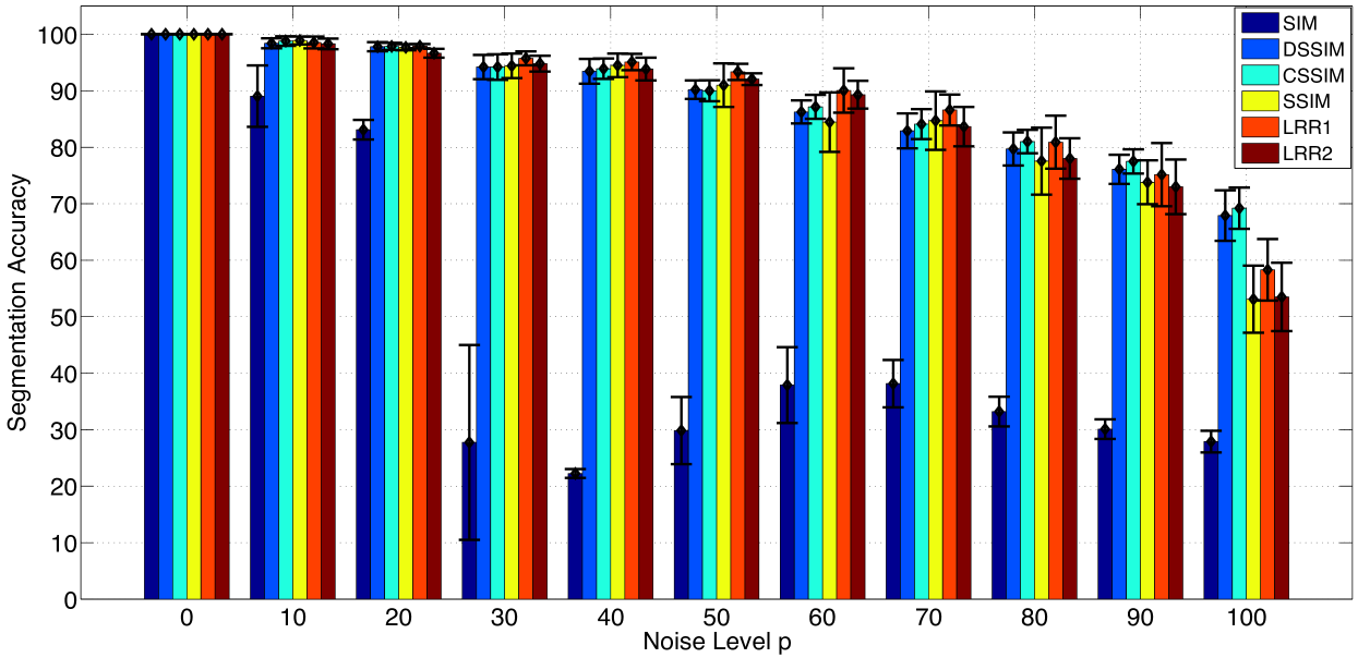
Figure 1: Results for synthetic data.

When $p=0$, i.e., in the ideal noiseless setting, all methods achieve perfect segmentation, as expected from Theorem 6. As we increase the noise level $p$, SIM degrades quickly since it has no protection against noise. LRR1 performs best in the range of $p=30\sim 70$, probably because its discrepancy measure matches the noise generation process the best. However, we note that the advantage of LRR1 over other methods is rather small. When most data points are corrupted ($p=80\sim 100$), DSSIM and CSSIM start to prevail. Overall, CSSIM, based on the trace norm regularizer, performs slightly better than SSIM, which is based on the Frobenius norm regularizer.

On the computational side, SIM, DSSIM, CSSIM and SSIM all have closed-form solutions and only require a single call to SVD, while LRR generally requires 300 steps to converge on this dataset; that is, 300 SVDs, since each step involves the SVD thresholding algorithm. Moreover, LRR pays extra computational cost in selecting the regularization constant. In total, LRR is orders of magnitude slower than all other methods.

We noted in experiments that if the noise magnitude is larger than a threshold, all methods will degrade to the level of SIM.

4.2 Hopkins155 Motion Segmentation

The hopkins155 dataset is a standard benchmark for motion segmentation and subspace clustering (Tron and Vidal,, 2007). It consists of 155 sequences of two or three motions. The motions in each sequence are regarded as subspaces while each sequence is regarded as a separate clustering problem, resulting in total 155 subspace clustering problems. The outliers in this dataset has been manually removed, hence we expect the independent subspace assumption to hold approximately. For a fair comparison, we apply all methods to the raw data, even though we have observed in experiments that the performances can be further improved by suitable preprocessing/postprocessing.

The results are tabulated in Table 1. All methods perform well on this dataset, even SIM achieves 75.56% accuracy, confirming that this dataset only contains small amount/magnitude of noise and obeys the independent subspace assumption reasonably well. The numbers in the “Mean” row are obtained by first averaging over all 155 sequences and then selecting the best out of the 9 regularization constants, with the best $\lambda$ tabulated below. The results are close to the state-of-the-art as reported in (Tron and Vidal,, 2007). If we are allowed to select the best $\lambda$ individually for each sequence, we obtain the “Best” row, which is surprisingly good. It is clear that LRR is significantly slower than all other methods. Note that the running time is not averaged over sequences, nor does it include the spectral clustering step or the tuning step.

Table 1: Segmentation Accuracy (%) on Hopkins155.

Method	SIM	DSSIM	CSSIM	SSIM	LRR1	LRR2
Mean	75.56	95.51	96.05	96.82	96.37	96.52
$\lambda$	0	$10^{-2}$	$10^{-3}$	$10^{-2}$	10	1
Time	3.56s	3.29s	3.61s	3.61s	695.1s	734.6s
Best	75.56	99.27	99.29	99.46	99.40	99.32

5 Conclusion

We have generalized the celebrated Eckart-Young-Mirsky theorem, under all unitarily invariant norms. Similar techniques are used to provide closed-form solutions for some interesting rank/norm regularized problems. The results are applied to subspace clustering, resulting in very simple algorithms. Experimental results demonstrate that the proposed algorithms perform comparably against the state-of-the-art in subspace clustering, but with a significant computational advantage.

Appendix: Proofs of the Main Results

Appendix A Preliminaries

We first re-establish some definitions from the main body. A matrix norm $\|\cdot\|$ is called unitarily invariant if $\|UAV\|=\|A\|$ for all $A\in\mathbb{M}^{m\times n}$ and all unitary matrices $U\in\mathbb{M}^{m\times m}$ and $V\in\mathbb{M}^{n\times n}$. We use $\|\cdot\|_{{\scriptscriptstyle\mathtt{UI}}}$ to denote unitarily invariant norms while $\|\cdot\|_{{\scriptscriptstyle\mathtt{AUI}}}$ means (simultaneously) all unitarily invariant norms. The notation $:=$ is used to indicate a definition.

As mentioned, the most important examples for unitarily invariant norms are perhaps:

$$\|A\|_{(k,p)}:=\Big{(}\sum_{i=1}^{k}\sigma_{i}^{p}\Big{)}^{1/p},$$ (20)

where $p\geq 1$, $k$ any natural number smaller than $\mathrm{rank}(A)$, and $\sigma_{i}$ is the $i$-th largest singular value of $A$. For $k=\mathrm{rank}(A)$, (20) is known as Schatten’s $p$-norm; while for $p=1$, it is called Ky Fan’s norm. Some special cases include the spectral norm ($p=\infty$), the trace norm ($p=1$, $k=\mathrm{rank}(A)$), and the Frobenius norm ($p=2$, $k=\mathrm{rank}(A)$). Note that all three norms belong to the Schatten’s family while only the first two norms are in the Ky Fan family. However, Ky Fan’s norm turns out to be very important in studying general unitarily invariant norms, due to the following fact (Theorem V.2.2, Bhatia, (1997)):

Lemma 1

$\|A\|_{{\scriptscriptstyle\mathtt{AUI}}}\leq\|B\|_{{\scriptscriptstyle\mathtt{AUI}}}$ iff $\forall k,\|A\|_{(k,1)}\leq\|B\|_{(k,1)}$.

Another interesting fact about unitarily invariant norms is (Problem II.5.5, Bhatia, (1997)):

Lemma 2

$$\Bigg{\|}\begin{pmatrix}A&B\\ C&D\end{pmatrix}\Bigg{\|}_{\mathtt{UI}}\geq\Bigg{\|}\begin{pmatrix}A&0\\ 0&D\end{pmatrix}\Bigg{\|}_{\mathtt{UI}}\geq\Bigg{\|}\begin{pmatrix}A&0\\ 0&0\end{pmatrix}\Bigg{\|}_{\mathtt{UI}}$$

Notice that Bhatia, (1997) assumes $A$ and $D$ to be square matrices. This assumption may be easily removed by padding with zeros. It is clear by induction that Lemma 2 can be extended to any number of blocks.

The following theorem is well-known and its proof can be found in Mirsky, (1960):

Theorem 1

Fix $\mathbb{N}\ni k\leq\mathrm{rank}(A)$, then $A_{(k)}$ is the minimum Frobenius norm solution of

$$\min_{X:~{}\mathrm{rank}{X}\leq k}\|A-X\|_{{\scriptscriptstyle\mathtt{AUI}}}.$$ (21)

The solution is unique iff the $k$-th and $(k+1)$-th largest singular values of $A$ differ.

Appendix B Proofs

We first prove the key proposition.

Proposition 2

If it exists, any minimizer of

$$\min_{X\in\mathcal{X}}\|X\|_{{\scriptscriptstyle\mathtt{AUI}}}$$ (22)

remains optimal for

$$\min_{X\in\mathcal{X}}\left\|\begin{pmatrix}X&0\\ 0&B\end{pmatrix}\right\|_{{\scriptscriptstyle\mathtt{AUI}}}$$

for any constant matrix $B$.

Proof: The proof is to repeatedly apply Lemma 1. Recall that the Ky Fan norm $\|\cdot\|_{(k,1)}$ defined in (20) is the sum of the $k$ largest singular values. Let $X^{\star}$ be an optimal solution of (22). According to Lemma 1, $\|X^{\star}\|_{(k,1)}\leq\|X\|_{(k,1)}$ for all admissible values of $k$ and for all feasible $X\in\mathcal{X}$. Then for all admissible values of $k$ and for all feasible $X\in\mathcal{X}$ we have:

$$\left\|\begin{pmatrix}X&0\\ 0&B\end{pmatrix}\right\|_{(k,1)} := \|X\|_{(k_{1},1)}+\|B\|_{(k_{2},1)}$$

$$\geq \|X\|_{(\hat{k}_{1},1)}+\|B\|_{(\hat{k}_{2},1)}$$

$$\geq \|X^{\star}\|_{(\hat{k}_{1},1)}+\|B\|_{(\hat{k}_{2},1)}$$

$$:= \left\|\begin{pmatrix}X^{\star}&0\\ 0&B\end{pmatrix}\right\|_{(k,1)},$$

where $k_{1}+k_{2}=\hat{k}_{1}+\hat{k}_{2}=k$ are suitable integers to fulfill the two definitions. Note that we have used the fact that the singular values of $\begin{pmatrix}X&0\\ 0&B\end{pmatrix}$ are precisely the union of singular values of $X$ and $B$. Applying Lemma 1 once more completes the proof. $\mbox{}\hbox{}\hfill\blacksquare$

For an arbitrary matrix $B$ with rank $r$, we denote its thin SVD as $B=U_{B}\Sigma_{B}V_{B}^{*}$. Define two projections $P_{B,\mathcal{L}}:=U_{B}U_{B}^{*}$ and $P_{B,\mathcal{R}}:=V_{B}V_{B}^{*}$. Let $U_{B}^{\perp}$ and $V_{B}^{\perp}$ be the orthogonal complements of $U_{B}$ and $V_{B}$, respectively.

Simultaneous Block Assumption (SB): Assume $(U_{B}^{\perp})^{*}AV_{C}=0$ and $U_{B}^{*}AV_{C}^{\perp}=0$.

Theorem 3

Fix $\mathbb{N}\ni k\leq\mathrm{rank}(A)$. Under the SB assumption, $B^{{\dagger}}(P_{B,\mathcal{L}}AP_{C,\mathcal{R}})_{(k)}C^{{\dagger}}$ is the minimum Frobenius norm solution of

$$\min_{X:~{}\mathrm{rank}{X}\leq k}\|A-BXC\|_{{\scriptscriptstyle\mathtt{AUI}}}.$$ (23)

The solution is unique iff the $k$-th and $(k+1)$-th largest singular values of $P_{B,\mathcal{L}}AP_{C,\mathcal{R}}$ differ.

Proof: Due to the SB assumption and the unitary invariance of the norm:

$$\|A-BXC\|_{{\scriptscriptstyle\mathtt{AUI}}}=\left\|\begin{pmatrix}\hat{A}-\Sigma_{B}\hat{X}\Sigma_{C}&0\\ 0&(U_{B}^{\perp})^{*}AV_{C}^{\perp}\end{pmatrix}\right\|_{{\scriptscriptstyle\mathtt{AUI}}},$$

where $\hat{A}=U_{B}^{*}AV_{C},\hat{X}=V_{B}^{*}XU_{C}$. It is apparent that $\mathrm{rank}(\hat{X})\leq\mathrm{rank}(X)\leq k$.

Next, by Proposition 2, we need only consider $\min\limits_{\mathrm{rank}(X)\leq k}\|\hat{A}-\Sigma_{B}\hat{X}\Sigma_{C}\|_{{\scriptscriptstyle\mathtt{AUI}}}$. Applying Theorem 1 we obtain $\Sigma_{B}\hat{X}\Sigma_{C}=(\hat{A})_{(k)}$. Since $\Sigma_{B}$ and $\Sigma_{C}$ are invertible, one can easily recover $X=V_{B}\Sigma_{B}^{-1}(\hat{A})_{(k)}\Sigma_{C}^{-1}U_{C}^{*}$ whose Frobenius norm is minimal (Penrose, (1956)). It is straightforward to verify that our choice of $X$ indeed simplifies to the form given in the theorem. The uniqueness property is inherited from Theorem 1. $\mbox{}\hbox{}\hfill\blacksquare$

Simultaneous Diagonal Assumption (SD): In addition to the SB assumption, assume furthermore $U_{B}^{*}AV_{C}$ is diagonal.

Theorem 4

Let $\lambda>0$. Under the SD assumption, the matrix problem

$$\min_{X}\|A-BXC\|_{{\scriptscriptstyle\mathtt{UI}}}+\lambda\cdot\|X\|_{{\scriptscriptstyle\mathtt{UI^{\prime}}}}$$ (24)

has an optimal solution of the form $X^{\star}=V_{B}\Sigma_{X}U_{C}^{*}$, with $\Sigma_{X}$ being diagonal.

Proof: Due to the SD assumption and the unitary invariance of the norm:

$$\|A-BXC\|_{{\scriptscriptstyle\mathtt{UI}}}=\left\|\begin{pmatrix}\hat{A}-\Sigma_{B}\hat{X}\Sigma_{C}&0\\ 0&(U_{B}^{\perp})^{*}AV_{C}^{\perp}\end{pmatrix}\right\|_{{\scriptscriptstyle\mathtt{UI}}},$$

where $\hat{A}=U_{B}^{*}AV_{C}$ and $\hat{X}=V_{B}^{*}XU_{C}$. Fix $X$ and define $\tilde{X}:=V_{B}YU_{C}^{*}$, where $Y$ is obtained by zeroing out all components of $\hat{X}$ except the diagonal. We now argue that $\tilde{X}$ has smaller objective value than $X$.

Due to unitary invariance:

$$\|\tilde{X}\|_{{\scriptscriptstyle\mathtt{UI^{\prime}}}} = \left\|\begin{pmatrix}Y&0\\ 0&0\end{pmatrix}\right\|_{{\scriptscriptstyle\mathtt{UI^{\prime}}}}$$

$$\leq \left\|\begin{pmatrix}V_{B}^{*}XU_{C}&0\\ 0&0\end{pmatrix}\right\|_{{\scriptscriptstyle\mathtt{UI^{\prime}}}}$$

$$\leq \|X\|_{{\scriptscriptstyle\mathtt{UI^{\prime}}}},$$

where the inequalities follow from Lemma 2. Since $\hat{A}$ is assumed diagonal, one can use similar arguments as in Proposition 2 to show that $\|A-B\tilde{X}C\|_{{\scriptscriptstyle\mathtt{UI}}}\leq\|A-BXC\|_{{\scriptscriptstyle\mathtt{UI}}}$.

Therefore we may restrict our attention to matrices in the form of $\tilde{X}:=V_{B}YU_{C}^{*}$, where $Y$ is everywhere zero except on its diagonal. But then (24) reduces to

$$\!\!\!\!\!\min_{y}\left\|\begin{pmatrix}\hat{A}-\Sigma_{B}\mathrm{diag}(y)\Sigma_{C}&0\\ 0&0\end{pmatrix}\right\|_{{\scriptscriptstyle\mathtt{UI}}}+\lambda\cdot\left\|\begin{pmatrix}\mathrm{diag}(y)&0\\ \!0&0\end{pmatrix}\right\|_{{\scriptscriptstyle\mathtt{UI^{\prime}}}},$$

which is a vector problem. $\mbox{}\hbox{}\hfill\blacksquare$

Theorem 5

Let $\lambda>0$. Then $\exists~{}r\in\{0,\ldots,\mathrm{rank}(\hat{A})\}$ such that $V_{B}(\hat{A}-\hat{A}_{(r)})U_{C}^{*}$ is the minimum Frobenius norm solution of

$$\min_{X}\mathrm{rank}(BAC-BXC)+\lambda\|X\|_{{\scriptscriptstyle\mathtt{RUI}}},$$ (25)

where $\|\cdot\|_{{\scriptscriptstyle\mathtt{RUI}}}$ is either the rank function or a unitarily invariant norm.

Proof: Let us first consider $\|\cdot\|_{{\scriptscriptstyle\mathtt{RUI}}}=\|\cdot\|_{{\scriptscriptstyle\mathtt{UI}}}$.

Step 1: Due to unitary and scaling invariance and Lemma 2, we have:

$$\mathrm{rank}[B(A-X)C] = \mathrm{rank}(\hat{A}-\hat{X}),$$

$$\lambda\|X\|_{{\scriptscriptstyle\mathtt{UI}}} \geq \lambda\|\hat{X}\|_{{\scriptscriptstyle\mathtt{UI^{\prime}}}},$$

where $\hat{X}=V_{B}^{*}XU_{C}$, and $\|\hat{X}\|_{{\scriptscriptstyle\mathtt{UI^{\prime}}}}:=\left\|\begin{pmatrix}\hat{X}&0\\ 0&0\end{pmatrix}\right\|_{{\scriptscriptstyle\mathtt{UI}}}$ is easily verified to be a unitarily invariant norm. Therefore we need only consider

$$\min_{\hat{X}}\mathrm{rank}(\hat{A}-\hat{X})+\lambda\|\hat{X}\|_{{\scriptscriptstyle\mathtt{UI^{\prime}}}}.$$

Step 2: We now argue that we may restrict $\hat{X}$ to have the same singular matrices as $\hat{A}$. Introduce $Z=\hat{A}-\hat{X}$ and consider

$$\min_{Z}\mathrm{rank}(Z)+\lambda\|\hat{A}-Z\|_{{\scriptscriptstyle\mathtt{UI^{\prime}}}}.$$

As indicated in Remark 2 in the main body of the paper, this rank regularized problem can be solved by considering a sequence of rank constrained problems. But, by Theorem 1, the optimal solution of each rank constrained problem can be chosen to have the same singular matrices as $\hat{A}$. Therefore the optimal $Z$, hence $\hat{X}$, can be so chosen as well.

Step 3: To determine the singular values of $\hat{X}$, we observe that unitarily invariant norms are always increasing functions of the singular values (Bhatia,, 1997). Given the value of $\mathrm{rank}(\hat{A}-\hat{X})$, say $r$, then $\tilde{X}:=\hat{A}-\hat{A}_{(r)}$ is easily seen to be optimal. But $r$ can only take a few integral values.

Step 4: Finally, given $\hat{X}$, we may easily recover $X=V_{B}\hat{X}U_{C}^{*}$ which is guaranteed to have minimum Frobenius norm (Penrose, (1956)). The proof for $\|\cdot\|_{{\scriptscriptstyle\mathtt{RUI}}}=\|\cdot\|_{{\scriptscriptstyle\mathtt{UI}}}$ is complete.

Now consider $\|\cdot\|_{{\scriptscriptstyle\mathtt{RUI}}}=\mathrm{rank}(\cdot)$. Step 1 clearly remains true, hence we need only consider

$$\min_{\hat{X}}\mathrm{rank}(\hat{A}-\hat{X})+\lambda\cdot\mathrm{rank}(\hat{X}).$$

Let $\hat{X}^{\star}$ be a minimizer with rank $(\mathrm{rank}(\hat{A})-r)$, then we see that $\tilde{X}:=\hat{A}-\hat{A}_{(r)}$ must also be optimal since

$$\mathrm{rank}(\tilde{X})=(\mathrm{rank}(\hat{A})-r)=\mathrm{rank}(\hat{X}^{\star}),$$

$$\mathrm{rank}(\hat{A}-\tilde{X})=r=\mathrm{rank}(\hat{A})-\mathrm{rank}(\hat{X}^{\star})\leq\mathrm{rank}(\hat{A}-\hat{X}^{\star}).$$

From the optimality of $\hat{X}^{\star}$ we also conclude that $\mathrm{rank}(\hat{A}-\hat{X}^{\star})=r$. But then $\tilde{X}$ must have smaller Frobenius norm than $\hat{X}^{\star}$ since the former is an optimal solution of

$$\min_{Y:~{}\mathrm{rank}(\hat{A}-Y)=r}\|Y\|_{{\scriptscriptstyle\mathtt{F}}},$$

while the latter is a feasible solution. $\mbox{}\hbox{}\hfill\blacksquare$

References

- Bhatia, (1997) Bhatia, R. (1997). Matrix Analysis. Springer.
- Cai et al., (2010) Cai, J.-F., Candès, E. J., and Shen, Z. (2010). A singular value thresholding algorithm for matrix completion. SIAM Journal on Optimization, 20(4):1956–1982.
- Costeira and Kanade, (1998) Costeira, J. P. and Kanade, T. (1998). A multibody factorization method for independently moving objects. International Journal of Computer Vision, 29(3):159–179.
- Eckart and Young, (1936) Eckart, C. and Young, G. (1936). The approximation of one matrix by another of lower rank. Psychometrika, 1(3):211–218.
- Elhamifar and Vidal, (2009) Elhamifar, E. and Vidal, R. (2009). Sparse subspace clustering. In IEEE conference on Computer Vision and Pattern Recognition, pages 2790–2797.
- Friedland and Torokhti, (2007) Friedland, S. and Torokhti, A. (2007). Generalized rank-constrained matrix approximations. SIAM Journal on Matrix Analysis and Applications, 29(2):656–659.
- Jolliffe, (2002) Jolliffe, I. T. (2002). Principal Component Analysis. Springer, 2nd edition.
- (8) Liu, G., Lin, Z., Yan, S., Sun, J., Yu, Y., and Ma, Y. (2010a). Robust recovery of subspace structures by low-rank representation. http://arxiv.org/pdf/1010.2955v3.
- (9) Liu, G., Lin, Z., and Yu, Y. (2010b). Robust subspace segmentation by low-rank representation. In International Conference on Machine Learning, pages 663–670.
- Luxburg, (2007) Luxburg, U. (2007). A tutorial on spectral clustering. Statistics and Computing, 17:395–416.
- Ma et al., (2011) Ma, S., Goldfarb, D., and Chen, L. (2011). Fixed point and bregman iterative methods for matrix rank minimization. Mathematical Programming, 128:321–353.
- Ma et al., (2007) Ma, Y., Derksen, H., Hong, W., and Wright, J. (2007). Segmentation of multivariate mixed data via lossy data coding and compression. IEEE Transactions on Pattern Analysis and Machine Intelligence, 29:1546–1562.
- Marshall et al., (2011) Marshall, A. W., Olkin, I., and Arnold, B. C. (2011). Inequalities: Theory of Majorization and Its Applications. Springer, 2nd edition.
- Mirsky, (1960) Mirsky, L. (1960). Symmetric gauge functions and unitarily invariant norms. Quarterly Journal of Mathematics, 11(2):50–59.
- Ni et al., (2010) Ni, Y. Z., Sun, J., Yuan, X., Yan, S., and Cheong, L.-F. (2010). Robust low-rank subspace segmentation with semidefinite guarantees. In ICDM Workshop on Optimization Based Methods for Emerging Data Mining Problems.
- Penrose, (1956) Penrose, R. (1956). On best approximate solutions of linear matrix equations. Mathematical Proceedings of the Cambridge Philosophical Society, 52(01):17–19.
- Piotrowski et al., (2009) Piotrowski, T., Cavalcante, R. L. G., and Yamada, I. (2009). Stochastic mv-pure estimator robust reduced-rank estimator for stochastic linear model. IEEE Transactions on Signal Processing, 57(4):1293–1303.
- Piotrowski and Yamada, (2008) Piotrowski, T. and Yamada, I. (2008). Mv-pure estimator minimum-variance pseudo-unbiased reduced-rank estimator for linearly constrained ill-conditioned inverse problems. IEEE Transactions on Signal Processing, 56(8):3408–3423.
- Seung and Lee, (2000) Seung, H. S. and Lee, D. D. (2000). The manifold ways of perception. Science, 290:2268–2269.
- Sondermann, (1986) Sondermann, D. (1986). Best approximate solutions to matrix equations under rank restrictions. Statistical Papers, 27:57–66.
- Tian, (2003) Tian, Y. (2003). Ranks of solutions of the matrix equation . Linear and Multilinear Algebra, 51(2):111–125.
- Tron and Vidal, (2007) Tron, R. and Vidal, R. (2007). A benchmark for the comparison of 3-d motion segmentation algorithms. In IEEE conference on Computer Vision and Pattern Recognition, pages 1–8.
- Vidal, (2011) Vidal, R. (2011). Subspace clustering. IEEE Signal Processing Magazine, 28(2):52–68.
- Vidal et al., (2005) Vidal, R., Ma, Y., and Sastry, S. (2005). Generalized principal component analysis (gpca). IEEE Transactions on Pattern Analysis and Machine Intelligence, 27:1945–1959.
- Zelnik-Manor and Irani, (2006) Zelnik-Manor, L. and Irani, M. (2006). On single-sequence and multi-sequence factorizations. International Journal of Computer Vision, 67(3):313–326.