Stabilized Lattice Boltzmann-Enskog method for compressible flows and its application to one and two-component fluids in nanochannels

Abstract

A numerically stable method to solve the discretized Boltzmann-Enskog equation describing the behavior of non ideal fluids under inhomogeneous conditions is presented. The algorithm employed uses a Lagrangian finite-difference scheme for the treatment of the convective term and a forcing term to account for the molecular repulsion together with a Bhatnagar-Gross-Krook relaxation term. In order to eliminate the spurious currents induced by the numerical discretization procedure, we use a trapezoidal rule for the time integration together with a version of the two-distribution method of He et al. (J. Comp. Phys 152, 642 (1999)). Numerical tests show that, in the case of one component fluid in the presence of a spherical potential well, the proposed method reduces the numerical error by several orders of magnitude. We conduct another test by considering the flow of a two component fluid in a channel with a bottleneck and provide information about the density and velocity field in this structured geometry.

I Introduction

Liquids often appear as homogeneous on a macroscopic scale, but not when observed on a microscopic scale where they may display density oscillations extending over a few molecular diameters. Equilibrium statistical mechanics theories such as density-functional theory (DFT) or integral equations can deal routinely with the presence of such inhomogeneities in density, concentration or other kinds of order parameters, and predict the ensemble average microscopic profiles and the associated surface and line tension, while a similar situation does not occur in non-equilibrium systems Evans ; hansen ; wu . In this case, the presence of inhomogeneities often causes difficulties in the numerical solution of the associated evolution equations.

It is well known that the conventional hydrodynamic description, based on the Navier-Stokes equation, faces difficulties when fluids are confined within a small volume or when the boundaries of the container have complicated shapes with typical lengths of the order of a few molecular diameters. Such a picture, while valid on a macroscopic scale, fails to describe very small systems NavierStokes ; Bruus ; Molecularphys2011 . On the other hand, the kinetic approach based on the distribution functions formalism and on the Boltzmann equation and its refinements represents a convenient description of both homogeneous and inhomogeneous systems. Among the existing numerical approaches employed to solve the Boltzmann equation, the Lattice Boltzmann (LB) method plays a prominent role LBgeneral ; LBmicro ; Ansumali . It is a discretized version of the continuous Boltzmann equation and gives good results in the homogeneous phases HeLuo ; HeLuo2 ; Abe . However, the numerical solution of inhomogeneous systems within the LB scheme is challenging: as reported by several authors Wagner ; Shan ; TOV ; Guo1 ; Pooley ; Zhang , a straightforward application of the LB equation leads to the observation of an unphysical effect, the so-called spurious currents, resulting from the discretization procedure. To cure this pathology, molecular interactions must be handled with care.

In the literature, internal forces are accounted for in two different ways: a) either by imposing the condition that the equilibrium distribution gives the desired form of the pressure tensor or b) by introducing an appropriate forcing term kikkinides ; Greci . The forcing term can be chosen in two different manners, either proportional to the gradient of the pressure excess over the ideal gas value or proportional to the product of the density times the gradient of the excess chemical potential, that is, by using the Gibbs-Duhem condition in differential form. Actually, the second choice is consistent with microscopic theories, such as DFT Evans , where the equilibrium condition is given by requiring that the gradient of the local chemical potential is locally balanced by the external forces.

In the present paper, we discuss a LBE algorithm based on the Boltzmann-Enskog transport equation vanbeijeren ; Santos ; Santos2 ; Lutsko ; Anero . The approach is particularly convenient when the packing effects are relevant, that is from moderate to high fluid densities. A straightforward application of the LBE algorithm leads to numerical instabilities so we introduce a numerical scheme that employs a trapezoidal time discretization plus an extension of a procedure, originally proposed by He et al. He , that uses two distribution functions, instead of one, to reduce the spurious currents phenomenon. In this scheme, one distribution function tracks the local density profile while the other tracks the local momentum density. The standard phase space distribution function $f({\bf r},{\bf v},t)$ is evolved concurrently with an auxiliary distribution function, named $g({\bf r},{\bf v},t)$, whose zeroth velocity-moment is the hydrodynamic pressure and its first moment is identical to the corresponding moment of $f({\bf r},{\bf v},t)$. According to previous authors, the reason for the increased stability of the double distribution method stems from the fact that the forcing term in the g-equation is multiplied by the difference between the local and the global Maxwellian thus reducing its importance with respect to the original f-equation, where the forcing term is multiplied by the local Maxwellian. The method was later extended and generalized by T. Lee and coworkers LeeLin ; LeeFischer ; Lee .

The main difference between our approach and the previous ones, besides the bottom-up microscopic modeling of the fluid proposed in earlier work Melchionna2008 ; Lausanne2010 ; JCP2007 , consists in the choice of the function employed to define the g-distribution function. As we shall see, with the present choice it is straightforward to generalize the method to multicomponent fluids, while in the original formulation such a generalization is not straightforward. In this way, our method leads naturally to a form of the forcing term similar to that in the Gibbs-Duhem route. This strategy can also be generalized to multicomponent fluids, whereas the pressure route cannot.

The paper is organized as follows: in Sec. II we present the evolution equation for the one particle distribution function $f$ and for the auxiliary distribution $g$ both for the simple fluid and for the fluid mixture. In Sec. III we discuss the discretization procedure In Sec. IV we present numerical tests of the proposed method. Finally in Sec. V we present our conclusions and perspectives.

II Equations for the double distribution functions

We start the discussion with the set of Boltzmann-Enskog equations characterizing a mixture of $M$ species, labelled with an upper index $\alpha=1,M$. The evolution equation for a particular distribution function $f^{\alpha}({\bf r},{\bf v},t)$ can be written as:

$$\frac{D}{Dt}f^{\alpha}({\bf r},{\bf v},t)=-\frac{{\bf F}^{\alpha}({\bf r})}{m}\cdot\frac{\partial}{\partial{\bf v}}f^{\alpha}({\bf r},{\bf v},t)+\sum_{\beta}J^{\alpha\beta}({\bf r},{\bf v},t)$$

(1)

where the material derivative is given by:

$$\frac{D}{Dt}=\frac{\partial}{\partial t}+{\bf v}\cdot\nabla.$$ (2)

and ${\bf F}^{\alpha}({\bf r})$ is an external velocity independent force field acting on component $\alpha$ and $J^{\alpha\beta}$, represents the effect on the single particle distribution function of the interactions among the fluid particles of type $\alpha$ and $\beta$.

Using a separation of the interaction term into a kinetic rapidly varying part and an hydrodynamic part originally introduced by Santos et al. Santos ; Santos2 and extended to mixtures later Melchionna2009 ; JCP2011 we rewrite (1) as:

$$\frac{Df^{\alpha}}{Dt}=-\omega(f^{\alpha}-f^{\alpha}_{eq})+S^{\alpha}_{f}({\bf r},{\bf v},t)$$ (3)

The first term in the r.h.s. of eq. (3) is a Bhatnagar-Gross-Krook (BGK) relaxation term BGK , $\omega$ an inverse relaxation time, and $S^{\alpha}_{f}$ is a source term due to external forcing and molecular interactions. According to JCP2011b it can be written as

$$S^{\alpha}_{f}({\bf r},{\bf v},t)=-\frac{{\bf F}^{\alpha}({\bf r})}{m}\frac{\partial}{\partial{\bf v}}f^{\alpha}+\beta({\bf v}-{\bf u})\cdot{\bf C}^{\alpha}({\bf r},t)\Gamma_{u}({\bf r},{\bf v},t)$$ (4)

with $\beta=1/k_{B}T$, $T$ is the temperature and $k_{B}$ the Boltzmann constant. In addition, $\Gamma_{u}$ is a Maxwellian velocity distribution whose mean velocity is the local fluid velocity ${\bf u}({\bf r},t)$:

$$\Gamma_{u}({\bf r},{\bf v},t)=\Bigl{(}\frac{1}{2\pi v_{T}^{2}}\Bigl{)}^{3/2}e^{-({\bf v}-{\bf u}({\bf r},t))^{2}/2v_{T}^{2}}$$ (5)

where $mv_{T}^{2}=k_{B}T$ for particles of common mass $m$, and

$$f^{\alpha}_{eq}({\bf r},{\bf v},t)=n^{\alpha}({\bf r},{\bf v},t)\Bigl{\{}1+\beta[({\bf u}^{\alpha}({\bf r},t)-{\bf u}({\bf r},t))\cdot({\bf v}-{\bf u}({\bf r},t))]\Bigl{\}}\Gamma_{u}({\bf r},{\bf v},t)$$ (6)

with ${\bf u}^{\alpha}$ the average velocity of the component $\alpha$. The term ${\bf C}^{\alpha}$ is a collisional kernel describing the change of $f^{\alpha}$ due to the interactions.

We first rewrite (3) in a form that is equivalent up to terms of third order in the Hermite expansion

$$S^{\alpha}_{f}=\beta\left({\bf C}^{\alpha}+n^{\alpha}\frac{{\bf F}^{\alpha}}{m}\right)\cdot({\bf v}-{\bf u})\Gamma_{u}.$$ (7)

From the phase space distribution function $f^{\alpha}({\bf r},{\bf v},t)$ we can compute the particle partial density,

$$n^{\alpha}({\bf r},t)=\int d{\bf v}f^{\alpha}({\bf r},{\bf v},t)$$ (8)

and the momentum current carried by particles of type $\alpha$,

$$n^{\alpha}({\bf r},t){\bf u}^{\alpha}({\bf r},t)=\int d{\bf v}f^{\alpha}({\bf r},{\bf v},t){\bf v}$$ (9)

which from eq. (3) satisfies the continuity equation

$$\frac{\partial n^{\alpha}}{\partial t}+\nabla\cdot(n^{\alpha}{\bf u}^{\alpha})=0.$$ (10)

The average fluid velocity is obtained from

$${\bf u}=\frac{\sum_{\alpha}n^{\alpha}{\bf u}^{\alpha}}{n}$$

with the global density given by

$$n=\sum_{\alpha}n^{\alpha}.$$

The numerical solution of eq. (3) is plagued by numerical instabilities as reported in ref. He , because the term $S^{\alpha}_{f}$ featured in the r.h.s. is quite large in the interfacial regions, since the main contribution to ${\bf C}^{\alpha}$, which is proportional to the gradient of the local chemical potential, varies rapidly. Alternatively, following the seminal idea put forward by He and coworkers in ref. He and pursued by Lee and coworkers Lee to stabilize the numerical solution the one component version of eq. (3), it is possible to employ an auxiliary distribution function, named $g^{\alpha}({\bf r},{\bf v},t)$ such that the role of the forcing term featured in its evolution equation is effectively reduced. Such an heuristic recipe stabilizes the numerical solution by "decoupling" the density and the momentum equations. In the present treatment, we will handle the stabilizing terms in an effective way, without relying on any heuristics. Let us introduce the auxiliary distribution

$$g^{\alpha}({\bf r},{\bf v},t)=f^{\alpha}({\bf r},{\bf v},t)+(\Pi^{\alpha}({\bf r},t)-n^{\alpha}({\bf r},t))\Gamma_{0}$$ (11)

where $\Pi^{\alpha}({\bf r},t)$ is a function of the partial densities , to be determined in the following, and $\Gamma_{0}$ indicates the velocity distribution at global equilibrium, that is, the Maxwellian corresponding to ${\bf u}=0$. One assumes that the function $\Pi^{\alpha}$ depends from its argument through $\{n^{\alpha}({\bf r},t)\}$. From the definition (11) one can see that $g^{\alpha}$ differs from $f^{\alpha}$ w.r.t. the zeroth moment

$$\int d{\bf v}g^{\alpha}({\bf r},{\bf v},t)=\Pi^{\alpha}({\bf r},t),$$ (12)

but shares the same first moment

$$\int d{\bf v}g^{\alpha}({\bf r},{\bf v},t){\bf v}=n^{\alpha}({\bf r},t){\bf u}^{\alpha}({\bf r},t).$$ (13)

By using eqs.(11) and (3), the evolution equation for $g^{\alpha}({\bf r},{\bf v},t)$ reads

$$\frac{Dg^{\alpha}}{Dt}=\frac{Df^{\alpha}}{Dt}+\frac{D}{Dt}(\Pi^{\alpha}-n^{\alpha})\Gamma_{0}.$$ (14)

$$\frac{D}{Dt}(\Pi^{\alpha}({\bf r},t)-n^{\alpha}({\bf r},t))=({\bf v}-{\bf u})\cdot\nabla(\Pi^{\alpha}-n^{\alpha})-\sum_{\beta}n^{\beta}(\frac{d\Pi^{\alpha}}{dn^{\beta}}-\delta_{\alpha\beta})\nabla\cdot{\bf u}^{\beta}-\sum_{\beta}(\frac{d\Pi^{\alpha}}{dn^{\beta}}-\delta_{\alpha\beta})({\bf u}^{\beta}-{\bf u})\cdot\nabla n^{\beta}$$ (15)

one obtains the evolution equation (14) for $g^{\alpha}({\bf r},{\bf v},t)$ as

$$\frac{Dg^{\alpha}}{Dt}=-\omega(g^{\alpha}-g^{\alpha}_{eq})+S^{\alpha}_{g}$$ (16)

with

$$S^{\alpha}_{g}({\bf r},t)=\beta\Bigl{(}{\bf C}^{\alpha}+n^{\alpha}\frac{{\bf F}^{\alpha}}{m}\Bigl{)}\cdot({\bf v}-{\bf u})(\Gamma_{u}-\Gamma_{0})$$

$$+\Bigl{[}\nabla\Pi^{\alpha}-\nabla n^{\alpha}+\beta{\bf C}^{\alpha}+n^{\alpha}\frac{{\bf F}^{\alpha}}{m}\Bigl{]}\cdot({\bf v}-{\bf u})\Gamma_{0}-\sum_{\beta}n^{\beta}(\frac{d\Pi^{\alpha}}{dn^{\beta}}-\delta_{\alpha\beta})(\nabla\cdot(n^{\beta}{\bf u}^{\beta})-{\bf u}\cdot\nabla n^{\beta})\Gamma_{0}$$ (17)

and

$$g^{\alpha}_{eq}({\bf r},{\bf v},t)=n^{\alpha}({\bf r},t)\Bigl{(}1+\beta m({\bf u}^{\alpha}({\bf r},t)-{\bf u}({\bf r},t))\cdot({\bf v}-{\bf u}({\bf r},t))\Bigl{)}\Gamma_{u}+(\Pi^{\alpha}({\bf r},t)-n^{\alpha}({\bf r},t))\Gamma_{0}.$$ (18)

It can be checked that the evolution equation for $g^{\alpha}$ or the one for $f^{\alpha}$ lead to the same balance equation for ${\bf u}^{\alpha}$. In practice, in the numerical work we shall use the $f^{\alpha}$ equation to determine the density $n^{\alpha}$ and track the formation of interfaces, and the $g^{\alpha}$ equation to determine the velocity field ${\bf u}^{\alpha}$.

The main motivation behind the transformation from $f^{\alpha}$ to $g^{\alpha}$ is that the effect of the forcing term, $S^{\alpha}_{g}$, featuring in (16) can be rendered smaller than the corresponding effect due to the forcing term, $S^{\alpha}_{f}$, in the original equation (3) for $f^{\alpha}$ by an appropriate choice of the function $\Pi^{\alpha}({\bf r},t)$. In fact, the first term in $S^{\alpha}_{g}$ is of order $({\bf v}-{\bf u})^{2}$ because it contains the product of $({\bf v}-{\bf u})(\Gamma_{u}-\Gamma_{0})$ , whereas the second term can be rendered small using the arbitrariness of the function $\Pi^{\alpha}$ is. As far as the last term is concerned we shall verify that the last term in $S^{\alpha}_{g}$ is actually small in our numerical simulation. One expects that a weaker forcing term helps the stability of the numerical solution. In the one component case He and coworkers suggested to replace $\beta^{-1}\Pi^{\alpha}$ by the thermodynamic pressure $p_{t}$. In order to see that we use the explicit representation of the function ${\bf C}^{\alpha}$, which represents the effect of the molecular interactions in the model studied.

We first separate the effective field ${\bf C}^{\alpha}$ into three separate contributions, the separation being quite generic and not determined by the particular model used:

$${\bf C}^{\alpha}({\bf r},t)={\bf C}^{\alpha,mf}({\bf r},t)+{\bf C}^{\alpha,drag}({\bf r},t)+{\bf C}^{\alpha,visc}({\bf r},t).$$ (19)

The first term can be written as:

$${\bf C}^{\alpha,mf}=-n^{\alpha}({\bf r},t)\nabla\mu_{int}^{\alpha}({\bf r},t).$$ (20)

where $\mu_{int}^{\alpha}$ is the non ideal part of the chemical potential of the $\alpha$ component. For density profiles smooth enough we can write

$${\bf C}^{\alpha,drag}({\bf r},t)\simeq-\gamma n^{\alpha}({\bf r},t)\sum_{\beta}({\bf u}^{\alpha}({\bf r},t)-{\bf u}^{\beta}({\bf r},t))$$ (21)

and for the viscous part

$$C_{i}^{\alpha,visc}({\bf r},t)\approx-n^{\alpha}({\bf r},t)\sum_{\beta}\Bigl{(}\eta^{\alpha\beta}\nabla^{2}u^{\beta}_{i}({\bf r},t)+(\eta^{\alpha\beta}_{b}+\frac{1}{3}\eta^{\alpha\beta})\nabla_{i}(\nabla\cdot{\bf u}^{\beta})\Bigl{)}$$ (22)

The coefficients $\gamma$ and $\eta$ depend on the specific model. In appendix A, we report their explicit representation for a system of hard-spheres with attractive interactions.

In the case of a one component fluid it is straightforward to derive the equation for the $g$ distribution which closely resembles the equation derived by He and coworkers. After dropping the unnecessary index $\alpha$ one has:

$$\frac{Dg}{Dt}=-\omega(g-g_{eq})+S_{g}$$ (23)

$$S_{g}=\beta({\bf C}+n\frac{{\bf F}}{m})\cdot({\bf v}-{\bf u})(\Gamma_{u}-\Gamma_{0})+\left[\nabla\Pi-\nabla n+\beta{\bf C}+n\frac{\beta{\bf F}}{m}\right]\cdot({\bf v}-{\bf u})\Gamma_{0}-n(\frac{d\Pi}{dn}-1)(\nabla\cdot{\bf u})\Gamma_{0}.$$

(24)

Using (20) and neglecting the non equilibrium contributions to ${\bf C}$ we have:

$$-\nabla n+\beta{\bf C}=-\beta n\nabla\mu$$ (25)

where $\mu$ is the total chemical potential. Finally with the help of the Gibbs-Duhem relation we introduce the thermodynamic pressure :

$$\nabla p_{t}=n\nabla\mu.$$ (26)

Hence, requiring the vanishing of the square brackets in (24) is equivalent to the condition:

$$\beta\nabla\Pi=\nabla p_{t}-n\frac{{\bf F}}{m}.$$ (27)

In other words choosing $\beta\Pi$ to be the thermodynamic potential augmented by the contribution due to the external field makes the second term of (24) to vanish. From the physical point of view such a condition is a consequence of the hydrostatic equilibrium condition Evans .

Unfortunately, in the multi-component fluid the identification of $\Pi^{\alpha}$ with the pressure is not possible. The reason is that in this case the distribution functions one needs a $\Pi^{\alpha}$ function for each component, whereas one can find only one pressure, through the Gibbs-Duhem relation

$$\nabla p_{t}=\sum_{\alpha}n^{\alpha}\nabla\mu^{\alpha}.$$ (28)

Moreover, by using the pressure route it is very difficult to obtain a satisfactory numerical solution in the general case, as in presence of confining walls, spontaneous layering mechanisms, or free interfaces. Alternatively, we choose the unknown function $\Pi^{\alpha}$ as the "potential function" associated with the vector field $\nabla n^{\alpha}-\beta{\bf C}^{\alpha}$, in such a way as to cancel this term from eq. (17). More precisely, the function $\Pi^{\alpha}$ is chosen to be:

$$\Pi^{\alpha}({\bf r},t)=n^{\alpha}({\bf r},t)-\beta\int^{{\bf r}}d{\bf r}^{\prime}\Bigl{(}{\bf C}^{\alpha,mf}({\bf r}^{\prime},t)+n^{\alpha}({\bf r}^{\prime},t)\frac{{\bf F}^{\alpha}({\bf r}^{\prime})}{m}\Bigl{)}$$ (29)

Therefore, being ${\bf C}^{\alpha,mf}$ a functional of density, $\Pi^{\alpha}$ is chosen to be a non-local function of density, in stark contrast with previous proposed approaches that are based on a local compensating pressure term He ; Lee ; Karni ; Karni2 . Eq. (29) also provides the operational route to our approach. In fact, the integral is evaluated numerically using trapezoidal spatial integration, which provides a satisfactory numerical solution in terms of accuracy. It should be noticed that, being an integral over a vector field, the integration depends on the origin and the specific path of the integral. However, this aspect is not dangerous for systems where a symmetry point can be found. In addition, the integration constant never appears in the evolution equation and thus does not need to be determined. Although eq. (16) looks more complicated than the original one, it behaves better in numerical terms and gives rise to smaller interfacial currents, as shown in the sequel.

III Numerical solution

We illustrate the numerical solution of the proposed method by considering explicitly the one component case, while the multicomponent case can be easily deduced. Let us consider again the integration of the generic evolution equation

$$\frac{Df}{Dt}=\Omega(f,M)({\bf r},{\bf v},t)$$ (30)

where the unspecified kernel $\Omega$ contains both the collisional term, the BGK term and the external force ${\bf F}\cdot\partial_{{\bf v}}f$. As customary in the derivation of the Lattice Boltzmann method, the distribution function is first projected on an finite Hermite basis set to handle the dependence on velocity shanyuanchen ; Moroni . By taking eq. (30) as our reference equation, the r.h.s. depends on $f$ but also on its moments $M=\{M_{p}\}$, with

$$M_{p}({\bf r},t)=<f|{\cal H}_{p}>$$ (31)

where ${\cal H}_{p}$ is the p-th Hermite polynomial, and

$$<A|{\cal H}_{p}>\equiv\int d{\bf v}A({\bf r},{\bf v},t){\cal H}_{p}({\bf v})$$ (32)

expresses the Hermite scalar product.

In order to discretize eq. (30), we start by considering the following truncated Hermite expansion

$$\bar{f}({\bf r},{\bf v},t)=\Gamma_{0}(v)\sum_{p=0}^{K}\frac{1}{v_{T}^{2p}2p!}M_{p}({\bf r},t){\cal H}_{p}({\bf v})$$ (33)

where $K$ is the order of truncation of the Hermite expansion and $M_{p}=<f|{\cal H}_{p}>=<\bar{f}|{\cal H}_{p}>$. In fact, from the definitions, it follows that the original and the truncated forms of the singlet distribution share the same moments up to $p\leq K$. By the same token, we consider the expansion of the collisional kernel,

$$\bar{\Omega}({\bf r},{\bf v},t)=\Gamma_{0}(v)\sum_{p=0}^{K}\frac{1}{v_{T}^{2p}p!}O_{p}({\bf r},t){\cal H}^{(p)}({\bf v})$$ (34)

with $O_{p}=<\Omega|{\cal H}^{(p)}>$. As for the distribution function, $\Omega$ has moments $O=\{O_{p}\}$ shared by the full and truncated representations of the kernel $\Omega$.

The LBM is based on replacing the Hermite scalar products by Gauss-Hermite quadratures to evaluate its moments,

$$M_{p}=<\bar{f}|{\cal H}_{p}>=\sum_{p=0}^{G}f_{p}{\cal H}^{(p)}({\bf c}_{p})$$ (35)

where the vectors ${\bf c}_{p}$ are a set of quadratures nodes, $w_{p}$ are the associated weights, and $G$ is the order of the quadratures.

The operational version of the LBM scheme is provided by the following quantities $f_{p}({\bf r},t)=w_{p}\bar{f}({\bf r},{\bf c}_{p},t)/\Gamma_{0}(c_{p})$ and $\Omega_{p}({\bf r},t)=w_{p}\overline{\Omega}({\bf r},{\bf c}_{p},t)/\Gamma_{0}(c_{p})$. From these transformations, the evolution equation of the new representation reads

$$\frac{\partial}{\partial t}f_{p}({\bf v},t)+{\bf c}_{p}\cdot\nabla f_{p}({\bf v},t)=\Omega_{p}(f_{p},M)({\bf r},t)$$ (36)

where we have rewritten the streaming term ${\bf v}\cdot\nabla f$ in its Hermite form. The exact time evolution of the populations over a timestep $h$ then reads

$$f_{p}({\bf r}+{\bf c}_{p}h,t+h)=f_{p}({\bf r},t)+\int_{t}^{t+h}ds\Omega_{p}(f_{p},M)({\bf r},s)$$ (37)

On the other hand, a second-order accurate $O(h^{2})$ numerical integration can be obtained via the trapezoidal rule rotenbergmoroni ,

$$\int_{t}^{t+h}ds\Omega_{p}(f_{p},M)({\bf r},s)=\frac{h}{2}\left[\Omega_{p}(f_{p},M)({\bf r}+{\bf c}_{p}h,t+h)+\Omega_{p}(f_{p},M)({\bf r},t)\right]+{\cal O}(h^{3})\equiv\frac{h}{2}\left(\Omega_{p}^{t+h}+\Omega_{p}^{t}\right)+{\cal O}(h^{3})$$ (38)

where $\Omega_{p}^{t}\equiv\Omega(f_{p},M)({\bf r},t)$.

Eq. (38) is apparently implicit. However, the scheme can be rendered explicit by using the following exact mapping to transform the original populations into the new set

$$\tilde{f}_{p}=f_{p}-\frac{\Omega_{p}(f_{p},M)}{2}h$$ (39)

The moments in the $\tilde{f}$ representation, collectively called $\tilde{M}_{p}=\{<\tilde{f}|{\cal H}_{p}>\}$, are related to those in the $f$ representation by

$$\tilde{M}_{p}=M_{p}-\frac{O_{p}}{2}h$$ (40)

In many circumstances, both relations eqs. (39)-(40) are invertible, that is, we can obtain explicitly the populations $f_{p}$ as a function of $\tilde{f}_{p}$ and the moments $M$ as a function of $\tilde{M}$. This is the case, for example, for BGK or Fokker-Planck kernels guo , and in presence of external forces.

Finally, the temporal evolution for the populations $\tilde{f}_{p}$ if given by the following updating scheme

$$\tilde{f}_{p}({\bf r}+{\bf c}_{p}h,t+h)=\tilde{f}_{p}({\bf r},t)+\Omega_{p}(f_{p},M)({\bf r},t)h$$ (41)

that provides the way to integrate the equation via the trapezoidal route. It is practical to work in the $\tilde{f}$ representation, and substitute the quantities $f_{p}$ and $M$ in the collisional kernel featuring in the r.h.s. of eq. (41).

For the collisional kernel $C$ appearing in eq. (3), however, the relation is non-invertible, since $C$ is a functional of the hydrodynamic moments. Yet, by decomposing $O(M)=O^{res}(M)+{\bf C}[M]$, where $O^{res}(M)$ is the residual part of the collisional moments, being a function (rather than a functional) of the hydrodynamic moments, a workable algorithm is obtained via the scheme

$$\tilde{M}_{p}=M_{p}-\frac{O_{p}^{res}(M)}{2}h-\frac{C_{p}[\tilde{M}]}{2}h$$ (42)

so that the original moments $M$ are expressed as functionals of $\tilde{M}$, and substituted in eq. (41). It is straightforward to show that, for $C=0$, the BGK and external forcing components give rise to the second-accurate integration method introduced by Guo et al. guo .

IV Results

In the following, we will analyze an ideal fluid with both the Euler integration, referred to as EU, and trapezoidal integration, referred to as TR. Subsequently, we will consider the hard-sphere system and compare the simulations obtained via the single distribution method (without the auxiliary distribution), named SD, and the double distribution method, named DD. By distinguishing the case of Euler integration from the trapezoidal integration, we have four combinations, for example, the double distribution method with the trapezoidal rule will be named DD-TR, and analogously for the other combinations, such as SD-EU, SD-TR and DD-EU.

IV.1 Ideal fluid in a potential well

To illustrate the numerical capabilities of the LBM, let us first consider an ideal fluid (by setting the collisional kernel $C=0$) in the presence of an external central potential, expressed as

$$U^{ext}=\left\{\begin{array}[]{c}-\epsilon(1+\cos(\frac{\pi r}{\xi}))\\ 0\end{array}\right.\;\begin{array}[]{c}\mbox{if}\;r<\xi\\ \mbox{else}\end{array}$$ (43)

where the potential depth is taken to be $\epsilon=0.3\times k_{B}T$ and the well size $\xi$ is varied in order to compare the standard Euler versus the trapezoidal integration rules. The external force is expressed as ${\bf F}^{ext}=-\nabla U^{ext}$ acting on particles of unit mass. At global equilibrium, the density should be distributed as $n^{eq}_{0}\exp(-U^{ext}/v_{T}^{2})$, with $n_{0}=\frac{1}{V}\int_{V}d{\bf r}n({\bf r})$, and the current should be zero everywhere.

By applying the trapezoidal rule, the populations $\tilde{f}_{p}$ are updated in time and, at every time step the density and current are computed as $\tilde{n}=\sum_{p}\tilde{f}_{p}$ and $\tilde{{\bf J}}=\sum_{p}{\bf c}_{p}\tilde{f}_{p}$. In the $f$ representation, the hydrodynamic moments that contain the second-order accuracy in space and time are computed by reversing equation (42), so that $n=\sum_{p}f_{p}=\tilde{n}$ and ${\bf J}=\sum_{p}{\bf c}_{p}f_{p}=\tilde{{\bf J}}+{\bf F}^{ext}\frac{h}{2}$.

Finally, the expression of the external forces up to second Hermite order, reads

$${\cal F}_{p}^{ext}=w_{p}\left[{\bf F}^{ext}\cdot{\cal H}_{p}^{(1)}+2{\bf F}^{ext}{\bf u}:{\cal H}_{p}^{(2)}\right]$$ (44)

where ${\cal H}_{p}^{(1)}={\cal H}^{(1)}({\bf c}_{p})=\frac{{\bf c}_{p}}{v_{T}^{2}}$ and ${\cal H}_{p}^{(2)}={\cal H}^{(2)}({\bf c}_{p})=\frac{{\bf c}_{p}{\bf c}_{p}-v_{T}^{2}{\bf I}}{2v_{T}^{4}}$, being a vector and a tensor of rank two, respectively, and ${\bf I}$ is the unit tensor.

By using eq. (41), it follows that $f_{p}=(1+\frac{\omega h}{2})^{-1}\times[\tilde{f}_{p}+\frac{\omega h}{2}f_{p}^{eq}+{\cal F}_{p}]$ and the populations are updated to the following post-collisional term

$$\tilde{f}_{p}^{*}=\tilde{f}_{p}+\frac{\omega h}{1+\omega h/2}\left[f_{p}^{eq}(n,{\bf u})-\tilde{f}_{p}\right]+\frac{h}{1+\omega h/2}{\cal F}_{p}^{ext}$$ (45)

to be contrasted with the standard Euler integration, reading

$$f_{p}^{*}=f_{p}+\omega h\left[f_{p}^{eq}(n,{\bf u})-f_{p}\right]+h{\cal F}_{p}^{ext}$$ (46)

Both the trapezoidal and Euler evolutions are then completed by the streaming stage, reading $\tilde{f}_{p}({\bf r}+h{\bf c}_{p},t+h)=\tilde{f}_{p}({\bf r},t)$ and $f_{p}({\bf r}+h{\bf c}_{p},t+h)=f_{p}({\bf r},t)$, respectively.

We simulate a three-dimensional system and in Fig. 1 we report the error on density as $Err(n)=\max_{{\bf r}}(|n-n^{eq}|/n_{0})$, the error on fluid velocity arising from parasitic effects, as $Err({\bf u})=\max_{{\bf r}}(|{\bf u}|/v_{T})$, and the error on current as $Err({\bf J})=\max_{{\bf r}}(|{\bf J}|/n_{0}v_{T})$. The data show that the numerical errors in the density, velocity and current decrease systematically with the mesh resolution for both the EU and TR methodologies. The error is reduced by about two orders of magnitude for the TR method as compared to the EU scheme. In particular, the error in density decreases as $\Delta x^{2}$ for both methods, while the error in current drops as $\Delta x^{2}$ and $\Delta x^{4}$ for the EU and TR methods, respectively. These preliminary results provide a reference for the subsequent simulations of the hard-sphere system and an important indication on the quality of the trapezoidal evolution method.

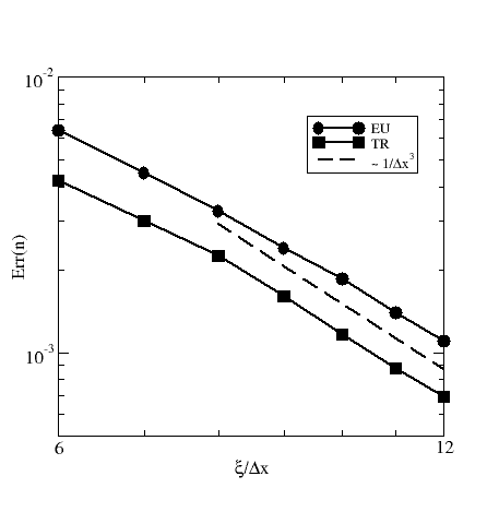
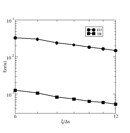
ABC

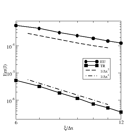
Figure 1: Numerical error in the density (panel A), velocity (panel B) and current (panel C) for the ideal gas system in presence of the central potential well. See text for details. The dashed and dot-dashed lines represent the power law dependence of the numerical error, as reported in the legends.

IV.2 Hard sphere fluid mixture in a potential well

We now consider a non ideal fluid mixture of hard spheres, and numerically solve the statics of the problem in the presence of the same central external potential of eq. (43), and integrate the dynamics with and without the auxiliary distribution method.

The trapezoidal integration for the two distributions generalizes eq. (41) to

$$\tilde{f}_{p}^{\alpha}({\bf r}+{\bf c}_{p}h,t+h) = \tilde{f}_{p}^{\alpha}({\bf r},t)+h\,\Omega_{f,p}^{\alpha}(f_{p}^{\alpha},\{M\})({\bf r},t)$$ (47)

$$\tilde{g}_{p}^{\alpha}({\bf r}+{\bf c}_{p}h,t+h) = \tilde{g}_{p}^{\alpha}({\bf r},t)+h\,\Omega_{g,p}^{\alpha}(g_{p}^{\alpha},\{N\})({\bf r},t)$$ (48)

where

$$\Omega_{f,p}^{\alpha}(f_{p},\{M\}) = \omega(f_{p}^{\alpha,eq}-f_{p}^{\alpha})+S_{f,p}^{\alpha}$$ (49)

$$\Omega_{g,p}^{\alpha}(g_{p},\{N\}) = \omega(g_{p}^{\alpha,eq}-g_{p}^{\alpha})+S_{g,p}^{\alpha}$$ (50)

Here, $\{M\}$ and $\{N\}$ refer to the set of moments of the populations $f_{p}^{\alpha}$ and $g_{p}^{\alpha}$ respectively.

We compute the relevant moments, that is, densities, HS chemical potentials and currents as

$$\tilde{n}^{\alpha} = \sum_{p}\tilde{f}_{p}^{\alpha}$$ (51)

$$\tilde{\Pi}^{\alpha} = \sum_{p}\tilde{g}_{p}^{\alpha}$$ (52)

$$\tilde{{\bf J}}^{\alpha} = \tilde{n}\tilde{{\bf u}}^{\alpha}=\sum_{p}{\bf c}_{p}\tilde{g}_{p}^{\alpha}$$ (53)

then

$$n^{\alpha} = \sum_{p}f_{p}^{\alpha}$$ (54)

$$\Pi^{\alpha} = \sum_{p}g_{p}^{\alpha}=\tilde{\Pi}^{\alpha}-\frac{h}{2}{\bf C}^{\alpha,mf}\cdot{\bf u}^{\alpha}$$ (55)

$${\bf J}^{\alpha} = n^{\alpha}{\bf u}^{\alpha}=\sum_{p}{\bf c}_{p}g_{p}^{\alpha}=\tilde{{\bf J}^{\alpha}}+\frac{h}{2}\left[{\bf C}^{\alpha,mf}+{\bf C}^{\alpha,visc}+n^{\alpha}{\bf F}^{\alpha}\right]$$ (56)

The explicit form of the r.h.s. of eqs. (49)-(50) reads

$$f_{p}^{\alpha,eq} = w_{p}\left[n^{\alpha}+n^{\alpha}{\bf u}^{\alpha}\cdot{\cal H}_{p}^{(1)}+n^{\alpha}(2{\bf u}^{\alpha}{\bf u}-{\bf u}{\bf u}):{\cal H}_{p}^{(2)}\right]$$ (57)

$$g_{p}^{\alpha,eq} = w_{p}\left[\Pi^{\alpha}+n^{\alpha}{\bf u}^{\alpha}\cdot{\cal H}_{p}^{(1)}+n^{\alpha}(2{\bf u}^{\alpha}{\bf u}-{\bf u}{\bf u}):{\cal H}_{p}^{(2)}\right]$$ (58)

$$S_{f,p}^{\alpha} = w_{p}\left\{\left({\bf C}^{\alpha,mf}+{\bf C}^{\alpha,visc}+n^{\alpha}{\bf F}^{\alpha}\right)\cdot\left[{\cal H}_{p}^{(1)}+2{\cal H}_{p}^{(2)}\cdot{\bf u}^{\alpha}\right]\right\}$$ (59)

$$S_{g,p}^{\alpha} = w_{p}\left\{{\bf C}^{\alpha,mf}\cdot\left[\frac{{\bf u}^{\alpha}}{v_{T}^{2}}+4{\cal H}_{p}^{(2)}\cdot{\bf u}^{\alpha}\right]+\left({\bf C}^{\alpha,visc}+n^{\alpha}{\bf F}^{\alpha}\right)\cdot\left[{\cal H}_{p}^{(1)}+2{\cal H}_{p}^{(2)}\cdot{\bf u}^{\alpha}\right]\right\}$$ (60)

In Fig. 2, the numerical error in the computed velocity profiles is reported for the one component and the two component fluids. The error decreases with increasing resolution and is smaller by respectively a factor $10$ and $50$ for the case of SD-TR and DD-TR simulations as compared to the SD-EU method. The data are similar for the one and two-component systems, follow the same behavior observed for the ideal gas, and the error in velocity decreases steadily with increasing resolution. The spurious velocities are about 50 times smaller for the DD-TR case as compared to the SD-EU integration.

A major advantage of the trapezoidal integration alone is the possibility to work at high packing fractions, up to about $0.35$, whereas with standard Euler integration, the maximal packing fraction before numerical instabilities develop is $0.27$.

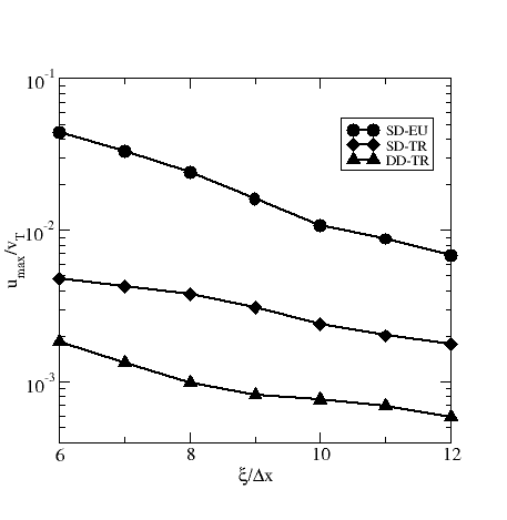
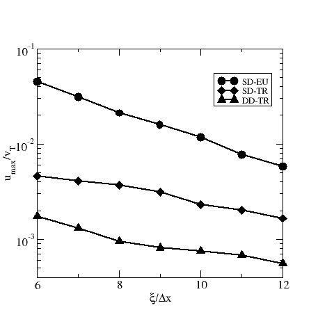
Figure 2: Numerical error in the fluid velocity in the presence of the central potential well for the one component fluid (left panel) and the binary mixture with diameters of $\sigma_{A}=4$ and $\sigma_{B}=8$ (right panel).

IV.3 Channel flow with a bottleneck

We now consider the flow of a one-component HS fluid and a binary mixture in a channel flow, in the presence of a bottleneck, as depicted in Fig. 3. Flows in the presence of a sharp obstacle represent a critical test to the numerical methodology due to the harsh collisions that the particles experience with the corners of the obstacle. In particular, we choose a rather strong forcing term, being equal to $10^{-3}$ in lattice units, in order to obtain large impinging velocities against the obstacle. We further impose no-slip boundary conditions on the fluid populations at the solid wall for both the $f$ and the $g$ distributions. For this we employ the mid-point bounce-back rule on the populations LBgeneral . We initially simulate a one-component system composed of hard spheres of diameter $\sigma=8$ and make complementary simulations with a two-component mixture with hard spheres diameters of $\sigma_{A}=4$ and $\sigma_{B}=8$.

As Fig. 4 demonstrates, the naive SD-EU method provides strong spurious velocities arising from the presence of the wall. In fact, away from the obstacle, the streamlines are expected to be parallel to the wall, whereas we observe strong non-parallel streamlines near the wall that confirm the low quality of this type of simulations. Conversely, the DD-TR method provides well aligned streamlines near the wall and far away from the bottleneck. From these observations, we decided to consider further benchmarks by looking at the results obtained with the DD-TR methodology alone.

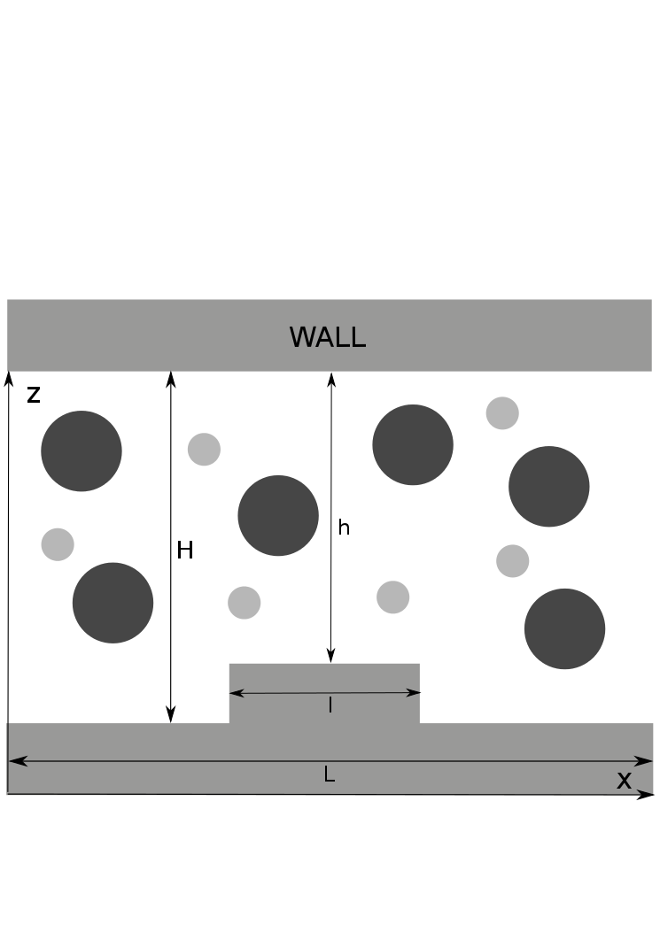
Figure 3: Sketch of the channel flow system in presence of an obstacle. The channel is filled with either a one-component fluid or a binary mixture. For the simulations we have set the geometry to $L=120$, $l=30$, $H=35$ and $h=28$ in lattice units. The diameters of the large and small particles are denoted $\sigma_{A}$ and $\sigma_{B}$, respectively.

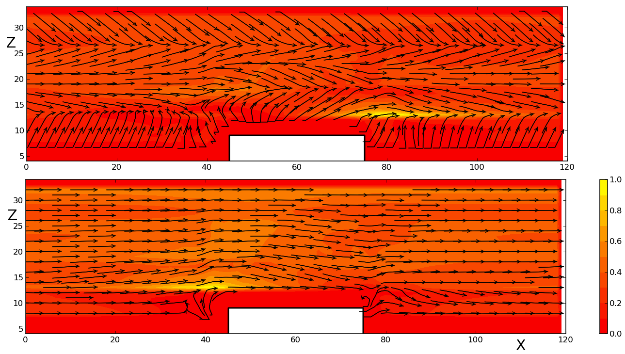
Figure 4: (Color online) One component system: comparison of streamlines for packing fractions of 0.13 as obtained with the SD-EU (upper panel) and with the DD-TR (lower panel) methods.

Hard spheres in proximity to an irregular surface present an interesting phenomenology in itself. In fact, in proximity to the obstacle, the fluid particles go around the obstacle with non-trivial patterns. In particular, as the flow lines in Fig. 5 reveal, a first bounce back is found near the convex corner. Entropic forces have a strong influence on the spatial distribution of the particles and, as previous studies demonstrate Dietrich , the concave corners effectively attract particles, while convex corners exert repulsive forces. Such dual behavior is recovered by our simulations, as revealed by the density profiles in Fig. 5 where the accumulation of particles toward the edges of the obstacle is clearly visible. In addition, we observe that the density profiles have a very weak dependence on the forcing term, with a somehow stronger variation in proximity of the corners for the incoming particles, as compared to the static case. A further validation of the method is given by the computation of the divergence of velocity, as reported in Fig. 6. For the compressible system considered here, the quantity $\nabla\cdot{\bf u}$ should be zero everywhere, while spurious compressibility effects are clearly visible when employing the SD-EU method. The DD-TR method minimizes such error up to three order of magnitudes.

For the system at hand, the simulations provide new interesting information about the fluid velocity in this geometry, as shown in the following.

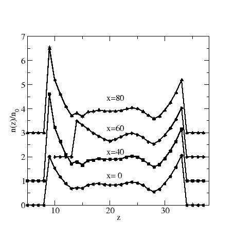
Figure 5: One component system: density profiles for different values of the x coordinate as obtained with and without forcing. The profiles for $x=40$ and $x=80$ correspond to positions right before and right after the corners of the obstacle. For all $x$ values, the profiles with and without forcing are basically indistinguishable. Profiles have been shifted upward for the sake of clarity.

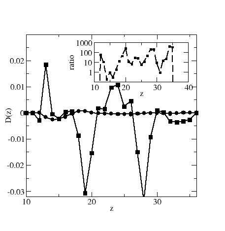
Figure 6: One component system: divergence of velocity $D\equiv\nabla\cdot{\bf u}/(v_{T}/\Delta x)$ computed at mid channel ($x=60$) for the system in flow condition. The two profiles correspond to the DD-TR (circle symbols) and SD-EU (square symbols) methods. The inset displays the ratio $|D^{DD-TR}/D^{SD-EU}|$.

The simulations provide the fine details of flow pattern for the one-component system at varying packing fraction, as illustrated in Fig. 7. For increasing packing fraction, the streamlines become more and more disordered in proximity to the convex corners of the bottleneck. A quite disordered pattern is observed already at a packing fraction of $0.26$, with flow separation appearing in correspondence with the impinged corner. The dynamical disorder appears to initiate at the far away edge of the obstacle with respect to the incoming flow direction. At a packing fraction of $0.34$, the disorder has propagated to the whole region of the bottleneck with rough recirculation patterns. It should be noticed that, for increasing packing fraction, the modulus of velocity is reduced overall, with strong peaks localized near the corners.

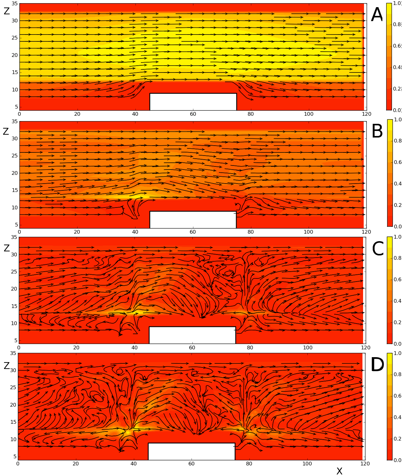
Figure 7: (Color online) One component system: streamlines for packing fractions of 0 (A panel), 0.13 (B panel), 0.26 (C panel) and 0.34 (D panel). The color map represents the modulus of the flow velocity, normalized by its maximum.

We have next considered a binary mixture of hard spheres of diameters $\sigma_{A}$ and $\sigma_{B}$, flowing in the same channel with the bottleneck. An important aspect of the binary mixture is that entropic forces play different roles on the species with different diameters. For particles of smaller diameter, entropic forces are smaller, and these particles can distribute more uniformly between the concave and convex corners. Consequently, the flow pattern is expected to be more ordered. This behavior is shown in Fig. 8, for a binary mixture with $\sigma_{A}=8$ and $\sigma_{B}=4$. The streamlines of both the large and small particles have a smoother behavior as compared to the one-component case. The modulus of velocity of both species is more uniform as compared to the one-component system, with a smoother distribution around the obstacle. In Fig. 9, the binary mixture with particles of size $\sigma_{A}=8$ and $\sigma_{B}=2$ presents even smoother flow lines and smoother distribution of the velocity moduli, as compared to simulations at smaller size ratio and at the corresponding packing fractions. Overall, we conclude that in the binary mixture, the component with particles of smaller size acts as a powerful lubricant that regularizes the flow pattern and distributes evenly the flow velocity over the whole system.

V Conclusions

In this paper, we have illustrated a numerical version of the Lattice Boltzmann method for the simulation of hard-sphere one-component and binary mixtures, that can deal with rapid spatial variations in the number density. As well-recognized in the Lattice Boltzmann community, strong inhomogeneities in the density induce strong parasitic currents that need to be handled with great care.

In our method, we have extended the previous ideas of He et al. He and T. Lee Lee but with some important modifications. In particular, we compute the excess chemical potential arising from the hard sphere collisions on-the-fly, without resorting to an educated guess of its functional form. In addition, we have adapted the trapezoidal integration rule for the time evolution of the populations, written as an explicit time-stepping algorithm.

The numerical results showed that, at all packing fractions considered in the benchmarks, the method provides robust results and stable numerical behavior.

We conclude by mentioning that the presented method can be applied without major modifications to nanofluids in presence of electrostatic interactions, as presented in ref. NOIEPL . For these systems, internal electrostatic forces exerted between charged species arise from the solution of a Poisson problem treated at mean-field, Vlasov level. Also in this case, the trapezoidal and double distribution methodology can be applied straightforwardly since electrostatic forces are treated at the same level of external forces.

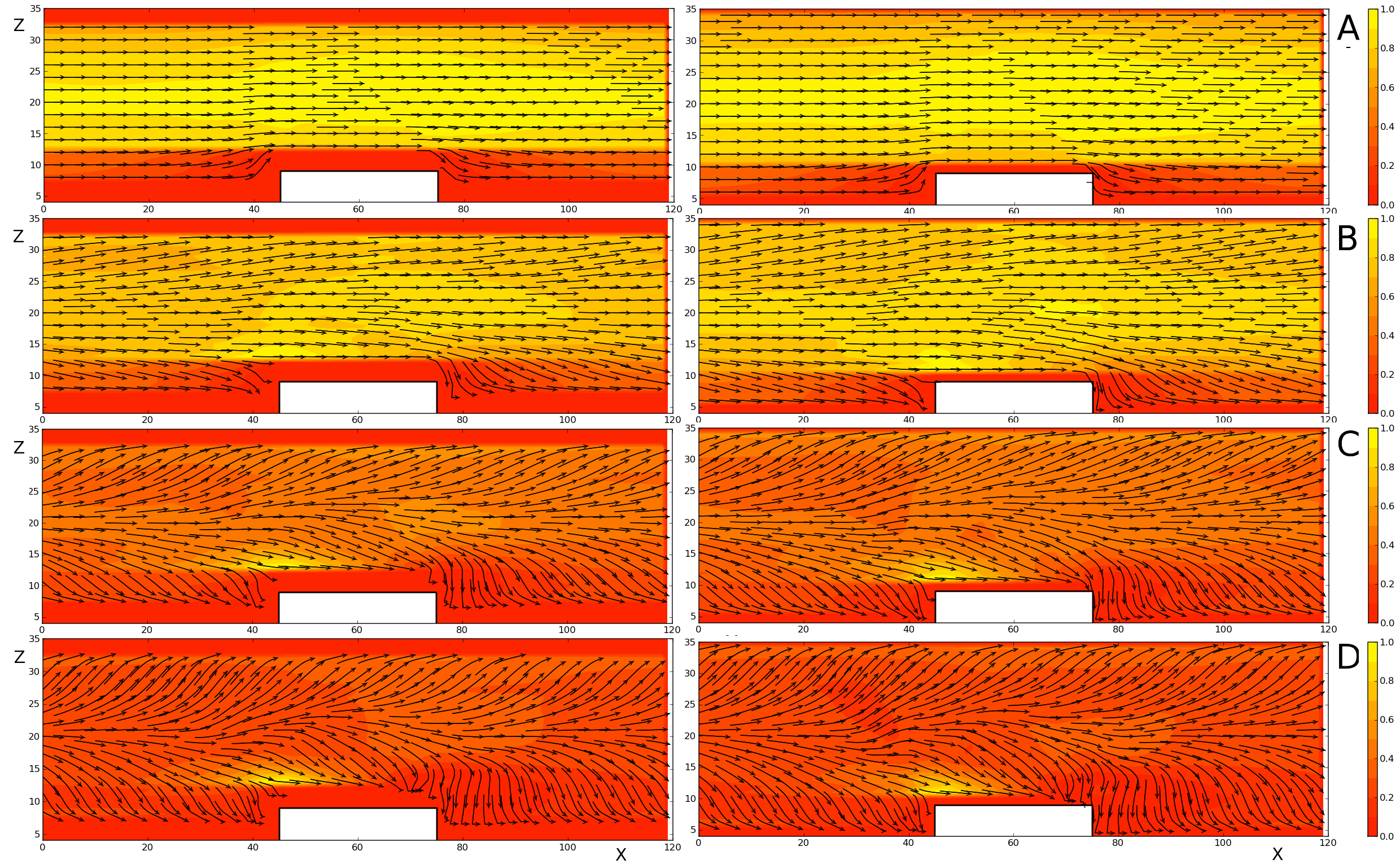
Figure 8: (Color online) Binary mixture with $\sigma_{A}=8$ (left column) and $\sigma_{B}=4$ (right column): streamlines for packing fractions of 0.0 (panel A), 0.13 (panel B), 0.26 (panel C) and 0.34 (panel D) and for 50% composition.

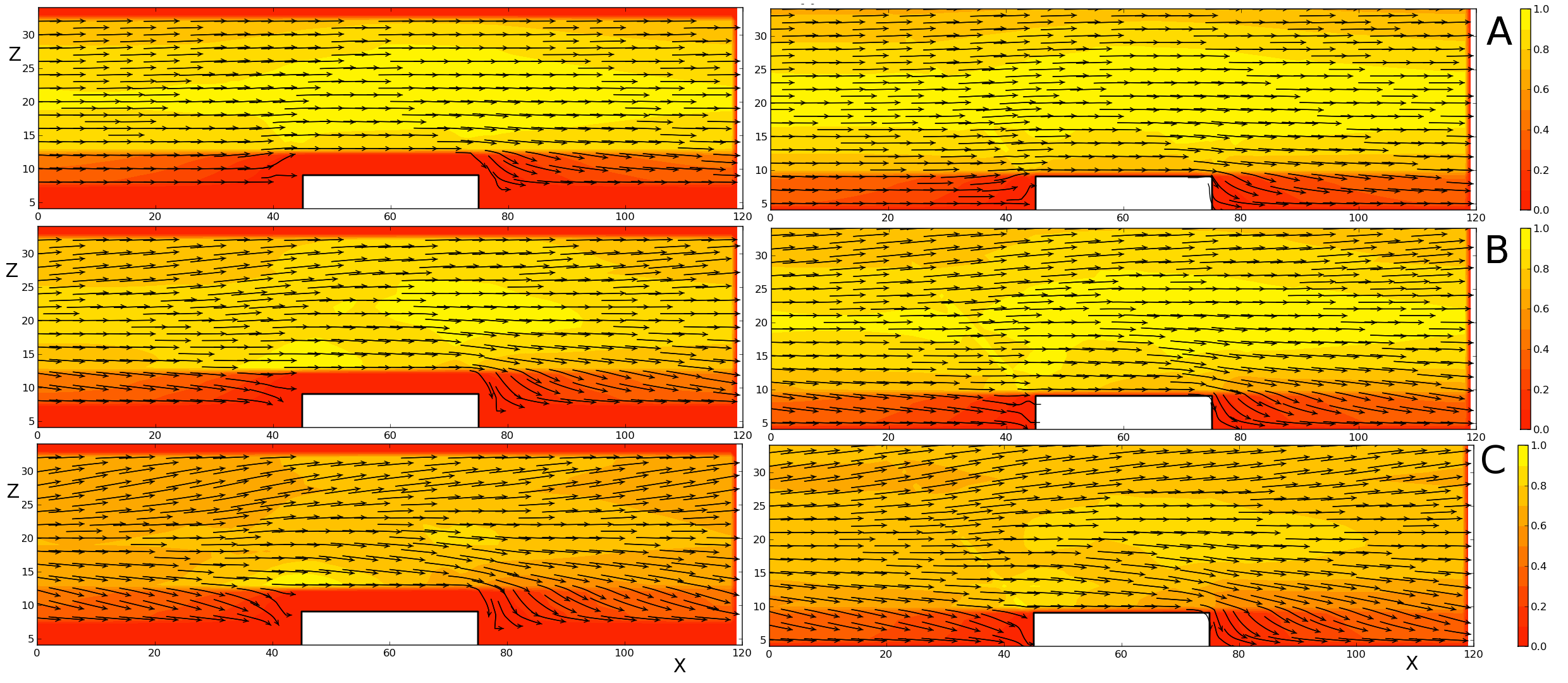
Figure 9: (Color online) Binary mixture with $\sigma_{A}=8$ (left column) and $\sigma_{B}=2$ (right column): streamlines for packing fractions of 0.13 (panel A), 0.26 (panel B) and 0.34 (panel C) and for 50% composition.

VI Appendix

We report the formulae given elsewhere which have been used to compute the various terms of the effective field. The details have been reported in a previous publication JCP2011 . In eq. (19) we can identify a force acting on the $\alpha$ particle at ${\bf r}$ due to the influence of all remaining particles in the system, the so called potential of mean force. For a hard-sphere mixture we have:

$${\bf C}^{\alpha,mf}({\bf r},t)=-k_{B}Tn^{\alpha}({\bf r},t)\sum_{\beta}\sigma_{\alpha\beta}^{2}\int d{\bf k}{\bf k}g_{\alpha\beta}({\bf r},{\bf r}+{\bf\sigma}_{\alpha\beta}{\bf k},t)n_{\beta}({\bf r}+{\bf\sigma}_{\alpha\beta}{\bf k},t)+n^{\alpha}({\bf r},t)\sum_{\beta}{\bf G}^{\alpha\beta}({\bf r},t)$$ (61)

with $\sigma_{\alpha\beta}=(\sigma_{\alpha\alpha}+\sigma_{\beta\beta})/2$, while the last term represents the molecular fields associated with the attractive forces:

$${\bf G}^{\alpha\beta}({\bf r},t)=-\int dr^{\prime}n^{\beta}({\bf r}^{\prime},t)g_{\alpha\beta}({\bf r},{\bf r}^{\prime})\nabla U^{\alpha\beta}({\bf r}-{\bf r}^{\prime})$$ (62)

with $U^{\alpha\beta}(r)$ a long range attractive potential. The drag term is:

$${\bf C}^{\alpha,drag}({\bf r},t)\simeq-n^{\alpha}({\bf r},t)\sum_{\beta}2\sigma_{\alpha\beta}^{2}\sqrt{\frac{k_{B}T}{\pi}}\frac{4\pi}{3}g_{\alpha\beta}(\{n^{\alpha}({\bf r},t)\})n^{\beta}({\bf r},t)({\bf u}^{\alpha}({\bf r},t)-{\bf u}^{\beta}({\bf r},t))$$ (63)

and for the viscous part

$${\bf C}^{\alpha,visc}({\bf r},t)=n^{\alpha}({\bf r},t)\sum_{\beta}2\sigma_{\alpha\beta}^{2}\sqrt{\frac{mk_{B}T}{\pi}}\int d{\bf k}{\bf k}g_{\alpha\beta}({\bf r},{\bf r}+{\bf\sigma}_{\alpha\beta}{\bf k},t)n^{\beta}({\bf r}+{\bf\sigma}_{\alpha\beta}{\bf k},t){\bf k}\cdot({\bf u}^{\beta}({\bf r}+{\bf\sigma}_{\alpha\beta}{\bf k})-{\bf u}^{\beta}({\bf r}))$$ (64)

where $g_{\alpha\beta}$ is the pair correlation function evaluated at contact ($r=\sigma_{\alpha\beta}$) As shown in Ref. JCP2011 one can derive the following expressions in the limit of a uniform system for the viscosity:

$$\eta^{\alpha\beta}=\frac{4\pi}{15}\sigma_{\alpha\beta}^{4}\sqrt{\frac{mk_{B}T}{\pi}}g_{\alpha\beta}n^{\beta}$$ (65)

and

$$\eta_{b}^{\alpha\beta}=\frac{5}{3}\eta^{\alpha\beta}$$ (66)

VI.1 Acknowledgments

We thank Jonas Lätt for drawing to our attention to ref. Lee and Benjamin Rotenberg for suggesting the use of the trapezoidal rule.

References

- (1) R. Evans, Adv. Phys. 28, 143 (1979).
- (2) J.P. Hansen and I.R. McDonald, Theory of Simple Liquids Academic Press, Oxford, (1990).
- (3) J. Wu and Z. Li, Annu. Rev. Phys. Chem. 58, 85, (2007).
- (4) Gad-el-Hak,J. Fluids Eng., 121, 5, (1999).
- (5) H. Bruus, Theoretical Microfluidics, Oxford University Pres., New York, 2008 .
- (6) U. Marini Bettolo Marconi, Mol. Phys., 109, 1265 (2011).
- (7) S. Succi, The Lattice Boltzmann equation for fluid dynamics and beyond, 1th edition , Oxford University Press, (2001).
- (8) J. Zhang, Microfluid Nanofluid 10, 1 (2001).
- (9) S. Ansumali, Commun. Comput. Phys. 9, 1106 (2011).
- (10) X. He, L.S. Luo, Phys. Rev. E 55, 6333 (1997).
- (11) X. He and L.S. Luo, J. Stat. Phys. 88, 927 (1997).
- (12) T. Abe, J. Comp. Phys 131, 241 (1997).
- (13) A.J. Wagner, International Journal of Modern Physics B, Volume 17, 193,(2003).
- (14) X. Shan, Phys. Rev. E 73, 047701 (2006).
- (15) M. Sbragaglia, R. Benzi, L. Biferale, S. Succi, K. Sugiyama and F. Toschi, Phys. Rev. E 75, 026702 (2007)
- (16) Z. Guo, C. Zheng and B. Shi, Phys. Rev. E 83, 036707 (2011).
- (17) C.M. Pooley and K. Furtado, Phys. Rev. E 77, 046702 (2008).
- (18) J. Zhang and F. Tian EPL 81 66005 (2008).
- (19) E.S.Kikkinides, A.G. Yiotis, M.E. Kainourgiakis and A.K. Stubos, Phys. Rev. E, 78, 036702 (2008).
- (20) E.S. Kikkinides, M.E. Kainourgiakis, A.G. Yiotis and A.K. Stubos, Phys. Rev.E, 82, 056705 (2010).
- (21) H. van Beijeren and M.H. Ernst, Physica A, 68, 437 (1973), 70, 225 (1973).
- (22) J. W. Dufty, A. Santos, and J.J. Brey, Phys. Rev. Lett. 77, 1270 (1996)
- (23) A.Santos, J.M. Montanero, J.W. Dufty and J.J. Brey, Phys.Rev. E 57, 1644 (1998).
- (24) J.F. Lutsko, Phys. Rev. Lett. 78, 243 (1997).
- (25) J. G. Anero and P. Espanol Europhysics. Lett. 78, 50005 (2007).
- (26) X. He, S. Chen and R. Zhang, J. Comp. Phys. 152, 642 (1999).
- (27) T. Lee and C.L. Lin, J. Comp. Phys. 206, 16 (2005) and Phys. Rev. E 67, 056703 (2003).
- (28) T. Lee and P. F. Fischer, Phys. Rev. E 74, 046709 (2006).
- (29) T. Lee, Computers and Mathematics with Applications 58, 987 (2009).
- (30) S. Karni, SIAM J. Sci. Comput. 17, 1019 (1996)
- (31) R. Abgrall and S. Karni, J. Comput. Phys. 169, 594 (2001).
- (32) S. Melchionna and U. Marini Bettolo Marconi, Europhys.Lett. 81, 34001 (2008).
- (33) U. Marini Bettolo Marconi and S.Melchionna, J.Phys.: Condens. Matter 36, 364110 (2010).
- (34) U. Marini Bettolo Marconi and S.Melchionna, J. Chem. Phys. 126, 184109 (2007).
- (35) U. Marini Bettolo Marconi and S.Melchionna, J. Chem. Phys. 131, 014105 (2009).
- (36) U. Marini Bettolo Marconi and S.Melchionna, J. Chem. Phys. 134, 064118 (2011).
- (37) P.L. Bhatnagar, E.P. Gross, and M. Krook, Phys. Rev. 94, 511 (1954).
- (38) U. Marini Bettolo Marconi and S.Melchionna, J. Chem. Phys. 135, 044104 (2011) .
- (39) D. Moroni, B. Rotenberg, J.-P. Hansen, S. Succi, S. Melchionna, Phys. Rev. E, 73, 066707 (2006).
- (40) X. Shan, X.-F. Yuan and H. Chen J.Fluid.Mech. 550, 413 (2006).
- (41) B. Rotenberg, D. Moroni, Phys. Rev. E, 74, 037701 (2006).
- (42) Z. Guo, C. Zheng, B. Shi, Phys. Rev. E, 65, 046308 (2002).
- (43) P. Bryk, R. Roth, M. Schoen and S. Dietrich, EPL 63 233 (2003).
- (44) S. Melchionna and U. Marini Bettolo Marconi, EPL 95 44002 ((2011).