Space-Constrained Interval Selection

Abstract

We study streaming algorithms for the interval selection problem: finding a maximum cardinality subset of disjoint intervals on the line. A deterministic $2$-approximation streaming algorithm for this problem is developed, together with an algorithm for the special case of proper intervals, achieving improved approximation ratio of $3/2$. We complement these upper bounds by proving that they are essentially best possible in the streaming setting: it is shown that an approximation ratio of $2-\epsilon$ (or $3/2-\epsilon$ for proper intervals) cannot be achieved unless the space is linear in the input size. In passing, we also answer an open question of Adler and Azar (J. Scheduling 2003) regarding the space complexity of constant-competitive randomized preemptive online algorithms for the same problem.

1 Introduction

In this paper we consider the interval selection problem, namely, finding a maximum cardinality subset of disjoint intervals from a given collection of intervals on the real line. It is well known that this problem has a simple optimal algorithm in the classical setting when the complete set of intervals is given to the algorithm [16]. Here we study this problem in the streaming model [18, 24], where the input is given to the algorithm as a stream of items (intervals in our case), one at a time, and the algorithm has a limited memory that precludes storing the whole input. Yet, the algorithm is still required to output a feasible solution, with a good approximation ratio.

The motivation for the streaming model stems from applications of managing very large data sets, such as biological data (DNA sequencing), network traffic data, and more. Although some function of the whole data set is to be computed, it is impossible to store the whole input. Depending on the setting, different variants of the streaming model have been considered in the literature, such as the classical streaming model [18] or the so-called semi-streaming model [13]. Common to all of them is the fact that the space used by the streaming algorithm is linear in some natural upper bound on the size of the output it returns (sometimes, a multiplicative polylogarithmic overhead is allowed).

In many problems considered in the streaming literature, the size of the output is fully determined by some parameter of the input, and thus, one would typically express the space complexity as a function of this parameter (cf. [4, 14]). However, in other problems, the size of the output cannot be a priori expressed that way as it depends on the given instance; in such settings it is natural to seek a streaming algorithm whose space complexity is not much larger than the output size of the given instance (cf. [17]). Clearly, as long as the computational model of the streaming algorithm is based on a Turing machine with no distinction between the working tape and the output tape, the size of the output is an inherent lower bound on the required space.

In this paper, we consider a setting where the algorithm is given a stream of real-line intervals, each one defined by its two endpoints, and the goal is to compute a maximum cardinality subset of disjoint intervals (or an approximation thereof). This problem finds many applications, e.g., in resource allocation problems, and it has been extensively studied in the online and offline settings in many variants. We seek algorithms with a good upper bound on the space they use for a given instance, expressed in terms of the size of the output for that specific instance. Typically, we seek algorithms that use space which is at most linear in the size of the output and yet guarantee a good approximation ratio.

Related Work.

The offline interval selection problem corresponds to finding a maximum independent set in an interval graph. An optimal greedy algorithm was discovered early [16] and has since been a staple of algorithms textbooks [9, 19]. It should be noted that the input can be given in (at least) two different ways: as an intersection graph with the nodes corresponding to the intervals, or as a set of intervals given by their endpoints. This distinction makes little difference in the traditional offline setting, where switching between these representations can be done efficiently, but, it can be important in access- or resource-constrained settings. We choose to study the interval selection problem assuming the latter representation — that is, the input is given as a set of intervals — since we believe that it makes more sense in applications related to the online and streaming settings (most previous works on online interval selection make the same choice).

The study of space-constrained algorithms goes back at least to the 1980 work of Munro and Paterson on selection and sorting [23]. More recently, the streaming model was developed to capture the processing of massive data-sets that arise in practice [24]. Most streaming algorithms deal with the approximate computation of various statistics, or “heavy hitters”, as exemplified by the celebrated paper of Alon, Matias, and Szegedy [4].

A number of classic graph theoretic problems have been treated in the streaming setting, for example, matching problems [22, 12], diameter and shortest paths [13, 14], min-cut [3], and graph spanners [14]. These were mostly studied under the semi-streaming model, introduced by Feigenbaum et al. [13]; in this model, the algorithm is allowed to use $n\log^{O(1)}(n)$ space on an $n$-vertex graph (i.e., $\log^{O(1)}(n)$ bits per vertex). Closest to our problem, the independent set problem in general sparse graphs (and hypergraphs) was studied in the streaming setting by Halldórsson et al. [17]. Geometric streaming algorithms have also appeared in recent years, especially dealing with extent and ranges, such as [2].

There is a plethora of literature on interval selection in the online setting. Some papers capture the problem as a call admission problem on a linear network, with the objective of maximizing the number (or weight) of accepted calls. Awerbuch et al. [5] present a strongly $\lceil\log N\rceil$-competitive algorithm for the problem, where $N$ is the number of nodes on the line (corresponding to the number of possible interval endpoints). This yields an $O(\log\Delta)$-competitive algorithm for the weighted case, where $\Delta$ is the ratio between the longest to the shortest interval. On the negative side, they establish a lower bound of $\Omega(\log N)$ on the competitive ratio of randomized non-preemptive online interval selection algorithms. In the context of the real line, this immediately implies that such algorithms cannot have a competitive ratio that is independent of the length of the input. In fact, Bachmann et al. [6] recently showed that the competitive ratio of randomized non-preemptive online algorithms for interval selection on the real line must be linear in the number of intervals in the input. Preemptive online scheduling has a lower bound of $\Omega(\log\Delta/\log\log\Delta)$ in the weighted case [8]. In comparison, much better results are possible for preemptive online algorithms in the unweighted setting: Adler and Azar [1] devise a $16$-competitive algorithm. One way of easing the task of the algorithm is to assume arrival by time, i.e., the intervals arrive in order of left endpoints. This has been treated for different weighted problems [25, 21, 11, 15].

Subsequent to the initial publication of the present results [10], Cabello and Pérez-Lanterno [7] gave streaming algorithms that estimate the size of the maximum independent set out of a set of intervals. Their algorithms give for a general instance a $(2+\epsilon)$ approximation, and for unit intervals a $(3/2+\epsilon)$ approximation, using space polynomial in $\frac{1}{\epsilon}$ and in $\log n$. They also gave new, simpler than ours, algorithms for finding the approximated independent set, which in some cases match our bounds as to the approximation ratio and the space used.

Our results.

We give tight results for the interval selection problem in the streaming setting. Our main positive result is a deterministic $2$-approximation streaming algorithm that uses space linear in the size of the output (Sec. 3). This is complemented by a matching lower bound (Sec. 5), stating that an approximation ratio of $2-\epsilon$ cannot be obtained by any randomized streaming algorithm with space significantly smaller than the size of the input (which can be much larger than the size of the output). The special case of proper interval collections (i.e., collections of intervals with no proper containments) is also considered, for which a deterministic $3/2$-approximation streaming algorithm that uses space linear in the output size is presented (Sec. 4) and a matching lower bound on the approximation ratio is established (Sec. 5) for streams of unit intervals (a special case of proper intervals). The upper bounds are extended to multiple-pass streaming algorithms: we show that an approximation ratio $1+1/(2p-1)$ can be obtained in $p$ passes over the input (Sec. 6).

In passing, we also answer an open question posed by Adler and Azar [1] in the context of randomized preemptive online algorithms for the interval selection problem. Adler and Azar point out that the decisions made by their online algorithm depend on the whole history (i.e., the input seen so far) and that natural attempts to remove this dependency seem to fail. Consequently, they write (using the term “active call” for an interval in the solution maintained by the online algorithm) that “it seems very interesting to find out whether there exist constant-competitive algorithms where each decision depends only on the currently active calls and maybe on additional bounded information”. We answer this question in the affirmative by slightly modifying our main algorithm to achieve a randomized preemptive online algorithm that admits constant competitive ratio and uses space linear in the size of the optimal solution, rather than the size of the input, as the algorithm of Adler and Azar does (Sec. 7).

2 Preliminaries

We think of the real line $\mathbb{R}$ as stretching from left to right so that an interval $I$ contains all points between its left endpoint $\mathrm{left}(I)$ and its right endpoint $\mathrm{right}(I)$, where $\mathrm{left}(I)<\mathrm{right}(I)$. Each endpoint can be either open (exclusive) or closed (inclusive). A half-open interval has a closed left endpoint and an open right endpoint. (This is, perhaps, the natural interval type to use in most resource allocation applications.) Observe that the assumption that $\mathrm{left}(I)<\mathrm{right}(I)$ implies that every interval contains an open set (in the topological sense) and that half-open intervals are always well defined.

The interval related notions of intersection, disjointness, and containment follow the standard view of an interval as a set of points. Two intervals $I,J$ properly intersect if they intersect without containment; $I$ properly contains $J$ if $I$ contains $J$ and $J$ does not contain $I$. An interval collection $\mathcal{I}$ is said to be proper (and the intervals in the collection, proper intervals) if no two intervals in $\mathcal{I}$ exhibit proper containment. The load of $\mathcal{I}$ is defined to be $\max_{p\in\mathbb{R}}|\{I\in\mathcal{I}\mid p\in I\}|$.

The interval selection problem asks for a maximum cardinality subset of pairwise disjoint intervals out of a given set $S$ of intervals. In the streaming model, the input interval set $S$ is considered to be an ordered set (a.k.a. a stream) and the intervals arrive one by one according to that order. The intervals are specified by their endpoints, where each endpoint is represented by a bit string of length $b$ (the same $b$ for all endpoints). This may potentially provide a streaming algorithm with the edge of knowing in advance some bounds on the number of intervals that will arrive and on the number of intervals that can be placed between two existing intervals. However, our algorithms do not take advantage of this extra information and our lower bounds show that it is essentially useless. An optimal solution to a given instance $S$ of the interval selection problem is denoted by $\mathtt{Opt}(S)$.

We may sometimes talk about segments, rather than intervals, when we want to emphasize that the entities under consideration are not necessarily part of the input. Given a set $\mathcal{I}$ of intervals, a component (or connected component) of $\mathcal{I}$ is a maximal continuous segment in $\bigcup_{I\in\mathcal{I}}I$.

3 The Main Algorithm

3.1 Overview

Given a stream $S$ of intervals, our algorithm maintains a (proper interval) collection $A\subseteq S$, referred to as the actual intervals, from which the output $\mathtt{Alg}(S)=\mathtt{Opt}(A)$ is taken. It also maintains a collection $V$ of virtual intervals, where each virtual interval is the intersection of two actual intervals that existed in $A$ at some point. The role of the virtual intervals is to prevent undesired intervals from joining $A$: an arriving interval $I\in S$ joins $A$ if and only if it does not contain any currently maintained virtual or actual interval.

Our algorithm is designed to guarantee that each interval $I\in S$ leaves a trace in either $A$ or $V$, namely, there exists some $J\in A\cup V$ such that $J\subseteq I$. Moreover, if $I,I^{\prime}\in A$ properly intersect, then $I\cap I^{\prime}\in V$. This essentially means that an arriving interval is rejected if and only if it contains some previous interval of $S$ or the intersection of two properly intersecting previous intervals in $S$ that have belonged to $A$.

Following that, it is not too difficult to show that the load of the interval collection $A$ is at most $2$. Based on a careful analysis of the structure of the (connected) components in $A$ and the locations of the virtual intervals within these components and between them, we can argue that $|V|\leq|A|$. This immediately yields the desired upper bound on the space of our algorithm as $|A|\leq 2\cdot|\mathtt{Opt}(A)|$. The bound on the approximation ratio essentially stems from the observation that $|\mathtt{Opt}(S)|\leq|\mathtt{Opt}(A\cup V)|$ (a direct corollary of the fact that each interval in $S$ leaves a trace in $A\cup V$) and from the invariant that each actual interval contains at most $2$ virtual intervals.

It is interesting to point out that our algorithm is in fact a deterministic preemptive online algorithm that maintains a load-$2$ interval collection (the collection $A$). Since the main result of Adler and Azar [1] also relies on such an algorithm, one may wonder if the two algorithms can be compared. Actually, the algorithm of Adler and Azar bases its rejection (and preemption) decisions on similar conditions: an arriving interval is rejected if and only if it contains some previous interval of $S$ or the intersection of two properly intersecting intervals in $A$. (Adler and Azar use a different terminology, but the essence is very similar.) The difference lies in the latter condition: Whereas the algorithm of Adler and Azar considers only the properly intersecting intervals that are currently in $A$, our algorithm also (implicitly) considers properly intersecting intervals that belonged to $A$ in the past and were preempted since. This seemingly small difference turns out to be crucial as it allows our algorithm to use much less memory, thus giving rise to an interesting phenomena: by remembering extra information (i.e., intersecting intervals that belonged to $A$ in the past and are not in $A$ anymore), we actually end up using less memory.

3.2 The algorithm

Consider a stream $S=(I_{1},\dots,I_{n})$ of intervals on the real line. It will be convenient to assume that all endpoints are distinct, i.e., $\{\mathrm{left}(I),\mathrm{right}(I)\}\cap\{\mathrm{left}(J),\mathrm{right}(J)\}=\emptyset$ for every two intervals $I,J\in S$. Unless stated otherwise, we will also assume that the intervals mentioned in this section are closed on both endpoints. These two assumptions are lifted in Appendix A.

Our algorithm, denoted $\mathtt{Alg}$, maintains a collection $A\subseteq S$ of actual intervals and a collection $V$ of virtual intervals, where each virtual interval is realized by endpoints of intervals in $S$. That is, the virtual interval $I\in V$ satisfies $\{\mathrm{left}(I),\mathrm{right}(I)\}\subseteq\{\mathrm{left}(J),\mathrm{right}(J)\mid J\in S\}$. The algorithm initially sets $A,V\leftarrow\emptyset$. Then, upon arrival of a new interval $I\in S$, $\mathtt{Alg}$ proceeds according to the policy presented in Algorithm 1.

Algorithm 1 The policy of $\mathtt{Alg}$ upon arrival of an interval $I\in S$.

1:  if $\exists J\in A\cup V$ s.t. $J\subseteq I$ then

2:     reject $I$ and halt

3:  $A\leftarrow A\cup\{I\}$

4:  for all $J\in A-\{I\}$ s.t. $J\supseteq I$ do

5:     $A\leftarrow A-\{J\}$

6:  for all $J\in V$ s.t. $J\supseteq I$ do

7:     $V\leftarrow V-\{J\}$

8:  for $p\in\{\mathrm{left}(I),\mathrm{right}(I)\}$ do

9:     if $\exists J\in V$ s.t. $p\in J$ then

10:        $V\leftarrow V-\{J\}\cup\{I\cap J\}$

11:     else if $\exists J\in A$ s.t. $p\in J$ then

12:        $V\leftarrow V\cup\{I\cap J\}$

13:  for all $J\in A$ and $K\in V$ do

14:     if $\mathrm{left}(J)<\mathrm{left}(K)<\mathrm{right}(K)<\mathrm{right}(J)$ then

15:        $A\leftarrow A-\{J\}$

The algorithm first verifies that the new interval $I$ does not contain any currently stored (actual or virtual) interval; if it does, then the new interval is ignored (rejected). Therefore, if $\mathtt{Alg}$ reaches line 3, then we can assume that $I\nsupseteq J$ for any interval $J\in A\cup V$. Next, in lines 4–7 $\mathtt{Alg}$ removes all the actual and virtual intervals that contain $I$. Lines 8–12 form the heart of the algorithm: updating the virtual intervals that remain in $V$. The idea here is that a virtual interval that intersects with $I$ is “trimmed” until it is contained in $I$; if an actual interval intersects with $I$, then the intersection is introduced as a new virtual interval. Finally, any actual interval $J$ that exclusively contains some virtual interval $K$ (that is, $J$ contains $K$ even if we remove $J$’s endpoints) is removed from the actual interval collection $A$ in lines 13–15.

After the last interval $I_{n}$ is processed, $\mathtt{Alg}$ outputs $\mathtt{Alg}(S)=\mathtt{Opt}(A)$, that is, an optimal subset of the interval collection $A$ (computed, say, by the greedy left-to-right algorithm). In the remainder of this section we prove that: (a) at all times, $|V|\leq|A|\leq 2\cdot|\mathtt{Alg}(S)|$; and (b) $|\mathtt{Alg}(S)|\geq|\mathtt{Opt}(S)|/2$. Together, we obtain the desired approximation, using space at most constant times larger than the size of the optimal output.

3.3 Analysis

Throughout the analysis, we let $1\leq t\leq n$ denote the time at which $\mathtt{Alg}$ completed processing interval $I_{t}\in S$; time $t=0$ denotes the beginning of the execution. We refer to the period between time $t-1$ and time $t$ as round $t$. The stream prefix $(I_{1},\dots,I_{t})$ is denoted by $S_{t}$. The collections $A$ and $V$ at time $t$ are denoted by $A_{t}$ and $V_{t}$, respectively, although, when $t$ is clear from the context, we may omit the subscript. We begin by showing that each virtual interval is indeed realized by (at most) two actual intervals and that the new interval $I$ is not removed immediately after joining $A$.

Proposition 3.1.

At any time $t$, we have $\{\mathrm{left}(\rho),\mathrm{right}(\rho)\mid\rho\in V_{t}\}\subseteq\{\mathrm{left}(\sigma),\mathrm{right}(\sigma)\mid\sigma\in S_{t}\}$.

Proof.

By induction on $t$. The case $t=0$ is trivial as $V_{0}=\emptyset$. For time $t>0$, we observe that any new virtual interval $\rho$ added to $V$ in round $t$ is either the intersection of two actual intervals (line 12) or the intersection of an actual interval and a virtual interval in $V_{t-1}$ (line 10). In the former case, the assertion follows immediately; in the latter case, the assertion follows by the inductive hypothesis. ∎

Proposition 3.2.

For every $1\leq t\leq n$, if $\mathtt{Alg}$ reaches line 3 when processing $I_{t}=I$, then $I\in A_{t}$.

Proof.

In line 3, $I$ is added to $A$ and subsequently, it can only be removed from $A$ if a virtual interval $\rho$ that is contained in $I$ but does not have an endpoint in common with $V$ is found (line 15). Such an interval $\rho$ cannot be in $V_{t-1}$ since otherwise, $I$ would have been rejected in line 2. The assertion follows since every virtual interval added to $V$ in round $t$ has a common endpoint with $I$. ∎

Lemma 3.3 lies at the core of our analysis: it states that each interval in $S$ leaves some trace in either $A$ or $V$. This will be employed later on to argue that $\mathtt{Alg}(S)$ is not much smaller than $\mathtt{Opt}(S)$.

Lemma 3.3.

For every interval $I_{t}\in S$ and for every time $t^{\prime}\geq t$, there exists some interval $\rho\in A_{t^{\prime}}\cup V_{t^{\prime}}$ such that $\rho\subseteq I_{t}$.

Proof.

A new coming interval $I$ is added to $A$ in line 3 unless some interval $\rho\subseteq I$ is found in $A\cup V$. An actual interval $\rho\in A$ is removed from $A$ only if another actual interval $I\subseteq\rho$ has just joined $A$ (line:5) or if a virtual interval $\sigma\subset\rho$ is found in $V$ (line:15). A virtual interval $\rho\in V$ is removed from $V$ only if an actual interval $I\subseteq\rho$ has just joined $A$ (line:7) or if it is replaced in $V$ by another virtual interval $\sigma\subseteq\rho$ (line 10). The assertion follows. ∎

3.3.1 The structural lemma

We now turn to establish our main lemma regarding the updating phase in lines 8–12 and the resulting structure of the interval collections $A$ and $V$. Lemma 3.4 states seven invariants maintained by our algorithm; these invariants are then proved simultaneously by induction on $t$, essentially by straightforward analysis of the policy presented in Algorithm 1.

Lemma 3.4.

For any round $1\leq t\leq n$, the updating phase satisfies the following two properties:
(P1) If $\rho$ is added to $V$ in round $t$, then $\rho\in V_{t}$.
(P2) If $\rho$ and $\sigma$ are added to $V$ in round $t$, then $\rho\cap\sigma=\emptyset$.
Moreover, for any time $0\leq t\leq n$, the interval collections $A$ and $V$ satisfy the following five properties:
(P3) For every $\rho\in A$ and $\sigma\in V$, if $\rho\cap\sigma\neq\emptyset$, then $\sigma\subset\rho$ with a common endpoint.
(P4) For every $\rho,\sigma\in A$, if $\rho\cap\sigma\neq\emptyset$, then $\rho\cap\sigma\in V$.
(P5) Every point $p\in\mathbb{R}$ is contained in at most $1$ virtual interval.
(P6) Every point $p\in\mathbb{R}$ is contained in at most $2$ actual intervals.
(P7) There do not exist two actual intervals $\rho,\sigma\in A$ such that $\rho\subseteq\sigma$.

Proof.

We first establish (P1) regardless of the other six properties.

Establishing (P1). It is sufficient to show that if $\rho$ is added to $V$ in line 10 or line 12 of the execution for $p=\mathrm{left}(I)$, then it is not removed from $V$ in line 10 of the execution for $p=\mathrm{right}(I)$. Indeed, if $\rho$ is added to $V$ in the execution for $p=\mathrm{left}(I)$, then $\rho=I\cap\sigma$ for some interval $\sigma\in A_{t-1}\cup V_{t-1}$ such that $\mathrm{left}(I)\in\sigma$. Since $\sigma$ cannot contain $I$ (as otherwise, it would have been removed in line 5 or line 7), it follows that $\mathrm{left}(\sigma)<\mathrm{left}(I)<\mathrm{right}(\sigma)<\mathrm{right}(I)$, so $\rho=[\mathrm{left}(I),\mathrm{right}(\sigma)]$. Therefore, $\mathrm{right}(I)\notin\rho$ and $\rho$ is not removed from $V$ in line 10 of the execution for $p=\mathrm{right}(I)$.

Next, we establish (P2), (P3), (P4), and (P5) simultaneously by induction on $t$. The case $t=0$ is trivial: (P2) holds vacuously, while (P3), (P4), and (P5) hold as $A_{0}=V_{0}=\emptyset$. Assume that the four properties hold for $t-1$ and consider the execution of $\mathtt{Alg}$ upon arrival of interval $I=I_{t}$ for some $1\leq t\leq n$.

Establishing (P2). As each iteration of the for loop in lines 8–12 adds at most one virtual interval to $V$, we may assume that $\rho$ is added in the execution for $p=\mathrm{left}(I)$ and $\sigma$ is added in the execution for $p=\mathrm{right}(I)$. This means that $\rho=I\cap\tau_{\ell}$ and $\sigma=I\cap\tau_{r}$ for some intervals $\tau_{\ell},\tau_{r}\in A_{t-1}\cup V_{t-1}$ such that $\mathrm{left}(I)\in\tau_{\ell}$ and $\mathrm{right}(I)\in\tau_{r}$. We argue that $\tau_{\ell}$ and $\tau_{r}$ do not intersect, which implies that $\rho$ and $\sigma$ do not intersect.

To that end, assume by way of contradiction that they do, and let $\tau_{\cap}=\tau_{\ell}\cap\tau_{r}$. If both $\tau_{\ell}$ and $\tau_{r}$ are virtual intervals, then we immediately reach a contradiction due the inductive hypothesis on (P5). If both $\tau_{\ell}$ and $\tau_{r}$ are actual intervals, which means that $\rho$ and $\sigma$ are added to $V$ in line 12, then by the inductive hypothesis on (P4), $\tau_{\cap}\in V_{t-1}$. By definition, $\tau_{\cap}$ must intersect with $I$. On the other hand, neither $\mathrm{left}(I)$ nor $\mathrm{right}(I)$ can belong to $\tau_{\cap}$ as otherwise, the else condition in line 11 would not have passed, thus $\tau_{\cap}\subset I$. But this means that $\mathtt{Alg}$ should not have reached line 3 and in particular, $\rho$ and $\sigma$ would not have been added to $V$.

So, assume that $\tau_{\ell}$ is actual and $\tau_{r}$ is virtual (the proof of the converse possibility is identical). By the inductive hypothesis on (P3), we know that $\tau_{r}\subset\tau_{\ell}$. But this implies that both endpoints of $I$ belong to $\tau_{\ell}$, namely, $I\subseteq\tau_{\ell}$, and $\tau_{\ell}$ should have been removed from $A$ in line 5.

Establishing (P3). Consider some $\rho\in A_{t}$ and $\sigma\in V_{t}$ such that $\rho\cap\sigma\neq\emptyset$. If $\rho\in A_{t-1}$ and $\sigma\in V_{t-1}$, then the property holds by the inductive hypothesis. Assume first that $\rho$ is added to $A$ in round $t$, so $\rho$ is the last arriving interval $I$. Notice that $\sigma$ cannot be in $V_{t-1}$ as this implies that either (i) $\sigma\subseteq I$, in which case $I$ would have been rejected in line 2; (ii) $\sigma\supseteq I$, in which case $\sigma$ would have been removed from $V$ in line 7; or (iii) $\sigma$ and $I$ properly intersect, in which case $\sigma$ is removed from $V$ in line 10. Thus, $\sigma$ is added to $V$ in round $t$ either in line 10 or in line 12. In both cases, $\sigma$ is contained in $I$ with a common endpoint.

It remains to consider the case in which $\rho\in A_{t-1}$ and $\sigma$ is added to $V$ in round $t$. If $\sigma$ is added to $V$ in line 10, then it replaces in $V$ some interval $\tau\in V_{t-1}$ such that $\sigma\subseteq\tau$. Hence, $\tau$ must also intersect with $\rho$ and by the inductive hypothesis, $\tau\subset\rho$, so $\sigma$ must be contained in $\rho$. Since $\rho$ is not removed in line 15, $\rho$ and $\sigma$ must have a common endpoint. If $\sigma$ is added to $V$ in line 12, then $\sigma=I\cap\tau$ for some interval $\tau\in A_{t-1}$ such that an endpoint $p$ of $I$ is contained in $\tau$. The property is established by arguing that $\tau$ and $\rho$ must be the same interval.

To that end, suppose toward a contradiction that $\tau\neq\rho$. Assume without loss of generality that $p=\mathrm{left}(I)$, so $\mathrm{left}(\tau)<\mathrm{left}(I)<\mathrm{right}(\tau)<\mathrm{right}(I)$. Since $\sigma=I\cap\tau=[\mathrm{left}(I),\mathrm{right}(\tau)]$ intersects with $\rho$, both $I$ and $\tau$ must also intersect with $\rho$. By the inductive hypothesis on (P4), we know that $\sigma_{\cap}=\rho\cap\tau\in V_{t-1}$. We also know that $\sigma_{\cap}$ intersects with $I$ as both $\rho$ and $\tau$ intersect with $I$. Since $\tau\nsupseteq I$, it follows that $\sigma_{\cap}\nsupseteq I$, hence $\sigma_{\cap}$ must still be in $V$ when $\mathtt{Alg}$ reaches line 8. If $\mathrm{left}(I)\in\sigma_{\cap}$, then the else condition in line 11 would not have passed and $\sigma$ would not have been added to $V$ in line 12, so $\mathrm{left}(I)\notin\sigma_{\cap}$. But $\mathrm{right}(I)\notin\sigma_{\cap}$ as $\mathrm{right}(I)\notin\tau$, hence $\sigma_{\cap}\subseteq I$ and $I$ should have been rejected in line 2. In any case, we conclude that $\rho$ and $\tau$ are indeed the same interval.

Establishing (P4). Consider two intersecting intervals $\rho,\sigma\in A_{t}$. If both $\rho$ and $\sigma$ are also in $A_{t-1}$, then by the inductive hypothesis, $\tau=\rho\cap\sigma\in V_{t-1}$. If $\tau\notin V_{t}$, then it must have been removed from $V$ either in line 7 because $I\subseteq\tau$, in which case $I$ is also contained in both $\rho$ and $\sigma$ and they would have been removed from $A$ in line 5, or in line 10, where it is replaced in $V$ by some other virtual interval $\tau^{\prime}\subset\tau$ (the strict containment follows from the distinct endpoints assumption), in which case at least one of the intervals $\rho$ and $\sigma$ should have been removed in line 15. Therefore, $\tau\in V_{t}$ and the property holds in that case.

So, suppose that $\rho\in A_{t-1}$, while $\sigma=I$ is added to $A$ in round $t$. Since $\rho,I\in A_{t}$, both $\rho$ and $I$ are in $A$ when $\mathtt{Alg}$ reaches line 8, thus they cannot contain each other. Assume without loss of generality that $\mathrm{left}(\rho)<\mathrm{left}(I)<\mathrm{right}(\rho)<\mathrm{right}(I)$. If $\mathrm{left}(I)$ does not belong to any virtual interval in $V_{t-1}$, then in line 12 the virtual interval $\tau=\rho\cap I$ is added to $V$ and it must still be there at time $t$ due to (P1). So, assume that $\mathrm{left}(I)$ belongs to some virtual interval $\tau\in V_{t-1}$. Since $\tau$ intersects with $\rho$, the inductive hypothesis on (P3) implies that $\tau\subset\rho$ with a common endpoint. In line 10, $\tau$ is replaced in $V$ by the new virtual interval $\tau^{\prime}=\tau\cap I$, which, by (P1) remains in $V$ at time $t$. The interval $\tau^{\prime}$ intersects with both $\rho$ and $I$, hence, by (P3) (applied to time $t$), it is contained in both of them, having a common endpoint with each, thus $\tau^{\prime}=\rho\cap\sigma$ and the property holds.

Establishing (P5). Suppose toward a contradiction that there exists two distinct intervals $\rho,\sigma\in V_{t}$ such that $\rho\cap\sigma\neq\emptyset$. Assume without loss of generality that $\sigma$ was added to $V$ after $\rho$. By the inductive hypothesis, $\sigma$ is added to $V$ in round $t$, while (P2) guarantees that $\rho\in V_{t-1}$. If $\sigma$ is added to $V$ in line 10, then $\sigma=I\cap\tau$ for some virtual interval $\tau$ which is guaranteed to be in $V_{t-1}$ by (P2). But then the inductive hypothesis implies that $\rho\cap\tau=\emptyset$, thus $\rho\cap\sigma=\emptyset$.

So, assume that $\sigma$ is added to $V$ in line 12. In that case $\sigma=I\cap\tau$ for some $\tau\in A_{t-1}$. Assume without loss of generality that $\mathrm{left}(\tau)<\mathrm{left}(I)<\mathrm{right}(\tau)<\mathrm{right}(I)$ so that $\sigma=[\mathrm{left}(I),\mathrm{right}(\tau)]$ is added to $V$ for $p=\mathrm{left}(I)$. Since $\rho$ intersects with $\sigma$, it must also intersect with both $I$ and $\tau$. We know that $p$ cannot belong to $\rho$ as otherwise, the else condition in line 11 would not have passed. But, by the inductive hypothesis on (P3), $\rho\subset\tau$, thus $\rho\subseteq I$ and $I$ should have been rejected in line 2.

Properties (P6) and (P7) can now be established based on the other properties.

Establishing (P6). Consider some point $p\in\mathbb{R}$ and suppose toward a contradiction that there exist three distinct intervals $\rho_{1},\rho_{2},\rho_{3}\in A_{t}$ such that $p\in\rho_{i}$ for every $1\leq i\leq 3$. By (P4), the intersections $\sigma_{1,2}=\rho_{1}\cap\rho_{2}$, $\sigma_{1,3}=\rho_{1}\cap\rho_{3}$, and $\sigma_{2,3}=\rho_{2}\cap\rho_{3}$ are all in $V_{t}$. But (P5) implies that $\sigma_{1,2}$, $\sigma_{1,3}$, and $\sigma_{2,3}$ are pairwise disjoint, in contradiction to their definition.

Establishing (P7). Consider any two intervals $\rho,\sigma\in A_{t}$. If $\rho\cap\sigma\neq\emptyset$, then (P4) implies that $\rho\cap\sigma\in V_{t}$. By (P3), $\rho\cap\sigma$ is strictly contained in both $\rho$ and $\sigma$, hence $\rho$ cannot be a subset of $\sigma$ (nor can $\sigma$ be a subset of $\rho$). ∎

3.3.2 The components

We employ Lemma 3.4 in order to understand the structure of the components of $A$ and their relations with the intervals in $V$. To that end, fix some time $t$ and consider an arbitrary component $C$ formed as the union of the actual intervals $\rho_{1},\dots,\rho_{k}\in A_{t}$. We denote the leftmost and rightmost points in (the segment) $C$ by $\mathrm{left}(C)$ and $\mathrm{right}(C)$, respectively.

Assume without loss of generality that $\mathrm{left}(\rho_{i})<\mathrm{left}(\rho_{i+1})$ for every $1\leq i\leq k-1$. Lemma 3.4(P6) and (P7) then guarantee that

$$\mathrm{left}(\rho_{i-1})<\mathrm{left}(\rho_{i})<\mathrm{right}(\rho_{i-1})<\mathrm{left}(\rho_{i+1})<\mathrm{right}(\rho_{i})<\mathrm{right}(\rho_{i+1})$$

for every $2\leq i\leq k-1$. By Lemma 3.4(P4), we conclude that $\rho_{i}\cap\rho_{i+1}\in V_{t}$ for every $1\leq i\leq k-1$, while Lemma 3.4(P3) implies that the segment $[\mathrm{left}(\rho_{2}),\mathrm{right}(\rho_{k-1})]$ does not intersect with any other virtual interval in $V_{t}$. The segment $C$ possibly contains two more virtual intervals at time $t$: an interval $\sigma_{\ell}\subseteq[\mathrm{left}(\rho_{1}),\mathrm{left}(\rho_{2}))$ and an interval $\sigma_{r}\subseteq(\mathrm{right}(\rho_{k-1}),\mathrm{right}(\rho_{k})]$, but then Lemma 3.4(P3) guarantees that $\mathrm{left}(\sigma_{\ell})=\mathrm{left}(\rho_{1})=\mathrm{left}(C)$ and $\mathrm{right}(\sigma_{r})=\mathrm{right}(\rho_{k})=\mathrm{right}(C)$. An illustration of a component is provided in Figure 1. There may also exist virtual intervals in between the components of $A$, but we will soon show that their number and structure are fairly limited. This requires the definition of the following notions.

Figure 1: A component $C$ of $A$. The solid lines depict the actual interval $\rho_{i}$, $i=1,\dots,5$; the dashed lines depict the virtual intervals that intersect with $C$ (all of them must be contained in $C$).

Partition into portions.

Point $p\in\mathbb{R}$ is said to be an $\langle{x,y}\rangle$-point at time $t$ if there exist exactly $x$ actual intervals in $A_{t}$ and $y$ virtual intervals in $V_{t}$ that contain $p$. By Lemma 3.4, it suffices to consider $\langle{x,y}\rangle$-points for $\langle{x,y}\rangle$ pairs in the set $\mathcal{F}=\{\langle{0,0}\rangle,\langle{1,0}\rangle,\langle{0,1}\rangle,\langle{1,1}\rangle,\langle{2,1}\rangle\}$, referred to as feasible pairs. Fixing some feasible pair $\langle{x,y}\rangle\in\mathcal{F}$, a maximal connected set of $\langle{x,y}\rangle$-points is referred to as an $\langle{x,y}\rangle$-portion. Given some segment $G\subseteq\mathbb{R}$, let $\varphi(G)$ be the string of feasible pairs that encodes the types of portions encountered in a left-to-right scan of $G$; e.g., if $C$ is the component illustrated in Figure 1, then $\varphi(C)=\langle{1,0}\rangle\,\langle{2,1}\rangle\,\langle{1,0}\rangle\,\langle{2,1}\rangle\,\langle{1,0}\rangle\,\langle{2,1}\rangle\,\langle{1,0}\rangle\,\langle{2,1}\rangle\,\langle{1,0}\rangle\,\langle{1,1}\rangle$.

More generally, it follows from Lemma 3.4 and the discussion above that for every component $C$ of $A$ it holds that

$$\varphi(C)\in\langle{1,1}\rangle^{?}\,\langle{1,0}\rangle\,(\langle{2,1}\rangle\,\langle{1,0}\rangle)^{*}\,\langle{1,1}\rangle^{?}\,,$$

where following the common notation in regular expressions, we use a superscript question mark to denote $0$ or $1$ occurrences and superscript asterisk to denote zero or more occurrences (cf. the Kleene star). Notice that by the distinct endpoints assumption, given $\varphi(C)$, it is easy to determine (uniquely) the numbers of actual and virtual intervals that $C$ contains and the relative (total) order of their endpoints. Thus the string $\varphi(C)$ gives the so-called topological structure of component $C$.

Likewise, if $P$ is a segment between two adjacent components of $A$, or the segment to the left of the leftmost component of $A$, or the segment to the right of the rightmost component of $A$, then it holds that

$$\varphi(P)\in\langle{0,0}\rangle\,(\langle{0,1}\rangle\,\langle{0,0}\rangle)^{*}\,.$$

We refer to the $\langle{0,1}\rangle$-portions as the isolated virtual intervals. The following lemma imposes a crucial restriction on the topological structure of $\varphi(P)$ (and also on $\varphi(C)$).

Lemma 3.5.

Let $\varphi_{t}=\varphi(\mathbb{R})$ be the string of feasible pairs that encodes the types of portions encountered in a left-to-right scan of the real line at time $1\leq t\leq n$. Then, every $\langle{0,0}\rangle$ entry in $\varphi_{t}$ is immediately preceded or immediately followed by a $\langle{1,0}\rangle$ entry.

Proof.

By induction on $t$. The assertion holds trivially for $t=1$ as $\varphi_{1}=\langle{0,0}\rangle\,\langle{1,0}\rangle\,\langle{0,0}\rangle$. Suppose that the assertion holds at time $t-1$ and consider time $t$. If $\mathtt{Alg}$ does not reach line 3 when processing $I=I_{t}$, then $\varphi_{t}=\varphi_{t-1}$ and the assertion holds by the inductive hypothesis, so assume hereafter that $\mathtt{Alg}$ does reach line 3 when processing $I$ which means that $I\nsupseteq J$ for any $J\in A_{t-1}\cup V_{t-1}$.

The proof continues by case analysis that considers the different types of possible intersections between $I$ and the portions corresponding to $\varphi_{t-1}$. Specifically, in Table 1 we identify a total of 27 types of intersections (up to symmetry) and address each one of them by depicting the string $\varphi_{t-1}$ together with a solid line stretched above the entries corresponding to the portions with which interval $I$ intersects. The resulting string $\varphi_{t}$ is given on the right column. The strings $\alpha,\beta\in\mathcal{F}^{*}$ are used to denote the substrings of $\varphi_{t-1}$ encoding the portions in segments of $\mathbb{R}$ which are (almost always) not affected by the newcoming interval $I$. We also use the notation

$$\alpha^{\prime}=\left\{\begin{array}[]{ll}\gamma,&\alpha=\gamma\,\langle{0,0}\rangle\\ \gamma\,\langle{x-1,y}\rangle,&\alpha=\gamma\,\langle{x,y}\rangle,\,x>0\end{array}\right.\qquad\beta^{\prime}=\left\{\begin{array}[]{ll}\gamma,&\beta=\langle{0,0}\rangle\,\gamma\\ \langle{x-1,y}\rangle\,\gamma,&\beta=\langle{x,y}\rangle\,\gamma,\,x>0\end{array}\right.$$

which facilitates a reduction in the number of cases we have to consider.

Observe that $I$ can interest at most $2$ elements of $A\cup V$, since otherwise $\exists J\in A\cup V$ s.t. $J\subseteq I$, and $I$ would not reach line 3 of the algorithm. Therefore, to cover all cases of the different types of possible intersections between $I$ and the portions corresponding to $\varphi_{t-1}$, Table 1 is divided into the following 5 main categories:

• C1: $I$ intersects with $0$ components of $A$ and with $0$ isolated virtual intervals.

• C2: $I$ intersects with $0$ components of $A$ and with $1$ isolated virtual interval.

• C3: $I$ intersects with $1$ component of $A$ and with $0$ isolated virtual intervals.

• C4: $I$ intersects with $1$ component of $A$ and with $1$ isolated virtual interval.

• C5: $I$ intersects with $2$ components of $A$ and with $0$ isolated virtual intervals.

For convenience, Category C3 is further divided into two parts, where the bottom part includes the cases where $I$ is included in the component $C$ of $A$ that $I$ intersects (i.e $I-C=\phi$,) and the top part includes the cases where $I-C\neq\phi$.

The assertion follows since in all cases, every $\langle{0,0}\rangle$ entry in $\varphi_{t}$ is immediately preceded or immediately followed by a $\langle{1,0}\rangle$ entry (taking into consideration the constraints imposed on $\alpha$ and $\beta$ due to the inductive hypothesis). ∎

category	$\varphi_{t-1}$	$\varphi_{t}$
C1	$\alpha\,\overline{\langle{0,0}\rangle}\,\beta$	$\alpha\,\langle{0,0}\rangle\,\langle{1,0}\rangle\,\langle{0,0}\rangle\,\beta$
C2	$\alpha\,\overline{\langle{0,0}\rangle\,\langle{0,1}\rangle}\,\langle{0,0}\rangle\,\beta$	$\alpha\,\langle{0,0}\rangle\,\langle{1,0}\rangle\,\langle{1,1}\rangle\,\langle{0,0}\rangle\,\beta$
	$\alpha\,\langle{0,0}\rangle\,\overline{\langle{0,1}\rangle}\,\langle{0,0}\rangle\,\beta$	$\alpha\,\langle{0,0}\rangle\,\langle{1,0}\rangle\,\langle{0,0}\rangle\,\beta$
C3	$\alpha\,\overline{\langle{1,0}\rangle\,\langle{0,0}\rangle}\,\beta$	$\alpha\,\langle{1,0}\rangle\,\langle{2,1}\rangle\,\langle{1,0}\rangle\,\langle{0,0}\rangle\,\beta$
	$\alpha\,\langle{1,0}\rangle\,\overline{\langle{1,1}\rangle\,\langle{0,0}\rangle}\,\beta$	$\alpha\,\langle{1,0}\rangle\,\langle{2,1}\rangle\,\langle{1,0}\rangle\,\langle{0,0}\rangle\,\beta$
	$\alpha\,\langle{0,0}\rangle\,\overline{\langle{1,1}\rangle\,\langle{1,0}\rangle\,\langle{0,0}\rangle}\,\beta$	$\alpha\,\langle{0,0}\rangle\,\langle{1,1}\rangle\,\langle{1,0}\rangle\,\langle{0,0}\rangle\,\beta$
	$\alpha\,\langle{1,0}\rangle\,\overline{\langle{2,1}\rangle\,\langle{1,0}\rangle\,\langle{0,0}\rangle}\,\beta$	$\alpha\,\langle{0,0}\rangle\,\langle{1,0}\rangle\,\langle{2,1}\rangle\,\langle{1,0}\rangle\,\langle{0,0}\rangle\,\beta$
	……………………………………	…………………………
	$\alpha\,\overline{\langle{1,0}\rangle}\,\beta$	$\alpha^{\prime}\,\langle{0,0}\rangle\,\langle{1,0}\rangle\,\langle{0,0}\rangle\,\beta^{\prime}$
	$\alpha\,\langle{1,0}\rangle\,\overline{\langle{1,1}\rangle}\,\langle{0,0}\rangle\,\beta$	$\alpha^{\prime}\,\langle{0,0}\rangle\,\langle{1,0}\rangle\,\langle{0,0}\rangle\,\beta$
	$\alpha\,\langle{1,0}\rangle\,\overline{\langle{2,1}\rangle}\,\langle{1,0}\rangle\,\beta$	$\alpha^{\prime}\,\langle{0,0}\rangle\,\langle{1,0}\rangle\,\langle{0,0}\rangle\,\beta^{\prime}$
	$\alpha\,\overline{\langle{1,0}\rangle\,\langle{1,1}\rangle}\,\langle{0,0}\rangle\,\beta$	$\alpha^{\prime}\,\langle{0,0}\rangle\,\langle{1,0}\rangle\,\langle{1,1}\rangle\,\langle{0,0}\rangle\,\beta$
	$\alpha\,\overline{\langle{1,0}\rangle\,\langle{2,1}\rangle}\,\langle{1,0}\rangle\,\beta$	$\alpha^{\prime}\,\langle{0,0}\rangle\,\langle{1,0}\rangle\,\langle{2,1}\rangle\,\langle{1,0}\rangle\,\beta$
	$\alpha\,\langle{0,0}\rangle\,\overline{\langle{1,1}\rangle\,\langle{1,0}\rangle\,\langle{1,1}\rangle}\,\langle{0,0}\rangle\,\beta$	$\alpha\,\langle{0,0}\rangle\,\langle{1,1}\rangle\,\langle{1,0}\rangle\,\langle{1,1}\rangle\,\langle{0,0}\rangle\,\beta$
	$\alpha\,\langle{1,0}\rangle\,\overline{\langle{2,1}\rangle\,\langle{1,0}\rangle\,\langle{1,1}\rangle}\,\langle{0,0}\rangle\,\beta$	$\alpha\,\langle{1,0}\rangle\,\langle{2,1}\rangle\,\langle{1,0}\rangle\,\langle{1,1}\rangle\,\langle{0,0}\rangle\,\beta$
	$\alpha\,\langle{1,0}\rangle\,\overline{\langle{2,1}\rangle\,\langle{1,0}\rangle\,\langle{2,1}\rangle}\,\langle{1,0}\rangle\,\beta$	$\alpha\,\langle{1,0}\rangle\,\langle{2,1}\rangle\,\langle{1,0}\rangle\,\langle{2,1}\rangle\,\langle{1,0}\rangle\,\beta$
C4	$\alpha\,\overline{\langle{1,0}\rangle\,\langle{0,0}\rangle\,\langle{0,1}\rangle}\,\langle{0,0}\rangle\,\beta$	$\alpha\,\langle{1,0}\rangle\,\langle{2,1}\rangle\,\langle{1,0}\rangle\,\langle{1,1}\rangle\,\langle{0,0}\rangle\,\beta$
	$\alpha\,\langle{0,0}\rangle\,\overline{\langle{1,1}\rangle\,\langle{1,0}\rangle\,\langle{0,0}\rangle\,\langle{0,1}\rangle}\,\langle{0,0}\rangle\,\beta$	$\alpha\,\langle{0,0}\rangle\,\langle{1,1}\rangle\,\langle{1,0}\rangle\,\langle{1,1}\rangle\,\langle{0,0}\rangle\,\beta$
	$\alpha\,\langle{1,0}\rangle\,\overline{\langle{2,1}\rangle\,\langle{1,0}\rangle\,\langle{0,0}\rangle\,\langle{0,1}\rangle}\,\langle{0,0}\rangle\,\beta$	$\alpha\,\langle{1,0}\rangle\,\langle{2,1}\rangle\,\langle{1,0}\rangle\,\langle{1,1}\rangle\,\langle{0,0}\rangle\,\beta$
C5	$\alpha\,\overline{\langle{1,0}\rangle\,\langle{0,0}\rangle\,\langle{1,0}\rangle}\,\beta$	$\alpha\,\langle{1,0}\rangle\,\langle{2,1}\rangle\,\langle{1,0}\rangle\,\langle{2,1}\rangle\,\langle{1,0}\rangle\,\beta$
	$\alpha\,\langle{1,0}\rangle\,\overline{\langle{1,1}\rangle\,\langle{0,0}\rangle\,\langle{1,0}\rangle}\,\beta$	$\alpha\,\langle{1,0}\rangle\,\langle{2,1}\rangle\,\langle{1,0}\rangle\,\langle{2,1}\rangle\,\langle{1,0}\rangle\,\beta$
	$\alpha\,\langle{0,0}\rangle\,\overline{\langle{1,1}\rangle\,\langle{1,0}\rangle\,\langle{0,0}\rangle\,\langle{1,0}\rangle}\,\beta$	$\alpha\,\langle{0,0}\rangle\,\langle{1,1}\rangle\,\langle{1,0}\rangle\,\langle{2,1}\rangle\,\langle{1,0}\rangle\,\beta$
	$\alpha\,\langle{0,0}\rangle\,\overline{\langle{1,1}\rangle\,\langle{1,0}\rangle\,\langle{0,0}\rangle\,\langle{1,1}\rangle}\,\langle{1,0}\rangle\,\beta$	$\alpha\,\langle{0,0}\rangle\,\langle{1,1}\rangle\,\langle{1,0}\rangle\,\langle{2,1}\rangle\,\langle{1,0}\rangle\,\beta$
	$\alpha\,\langle{0,0}\rangle\,\overline{\langle{1,1}\rangle\,\langle{1,0}\rangle\,\langle{0,0}\rangle\,\langle{1,0}\rangle\,\langle{1,1}\rangle}\,\langle{0,0}\rangle\,\beta$	$\alpha\,\langle{0,0}\rangle\,\langle{1,1}\rangle\,\langle{1,0}\rangle\,\langle{1,1}\rangle\,\langle{0,0}\rangle\,\beta$
	$\alpha\,\langle{1,0}\rangle\,\overline{\langle{2,1}\rangle\,\langle{1,0}\rangle\,\langle{0,0}\rangle\,\langle{1,0}\rangle}\,\beta$	$\alpha\,\langle{1,0}\rangle\,\langle{2,1}\rangle\,\langle{1,0}\rangle\,\langle{2,1}\rangle\,\langle{1,0}\rangle\,\beta$
	$\alpha\,\langle{1,0}\rangle\,\overline{\langle{2,1}\rangle\,\langle{1,0}\rangle\,\langle{0,0}\rangle\,\langle{1,1}\rangle}\,\langle{1,0}\rangle\,\beta$	$\alpha\,\langle{1,0}\rangle\,\langle{2,1}\rangle\,\langle{1,0}\rangle\,\langle{2,1}\rangle\,\langle{1,0}\rangle\,\beta$
	$\alpha\,\langle{1,0}\rangle\,\overline{\langle{2,1}\rangle\,\langle{1,0}\rangle\,\langle{0,0}\rangle\,\langle{1,0}\rangle\,\langle{1,1}\rangle}\,\langle{0,0}\rangle\,\beta$	$\alpha\,\langle{1,0}\rangle\,\langle{2,1}\rangle\,\langle{1,0}\rangle\,\langle{1,1}\rangle\,\langle{0,0}\rangle\,\beta$
	$\alpha\,\langle{1,0}\rangle\,\overline{\langle{2,1}\rangle\,\langle{1,0}\rangle\,\langle{0,0}\rangle\,\langle{1,0}\rangle\,\langle{2,1}\rangle}\,\langle{1,0}\rangle\,\beta$	$\alpha\,\langle{1,0}\rangle\,\langle{2,1}\rangle\,\langle{1,0}\rangle\,\langle{2,1}\rangle\,\langle{1,0}\rangle\,\beta$

Table 1: The different types of intersections of interval $I$ with the portions corresponding to $\varphi_{t-1}$ and the resulting $\varphi_{t}$.

3.3.3 Accounting

We are now ready to establish the following lemma.

Lemma 3.6.

$|\mathtt{Alg}(S_{t})|\geq|\mathtt{Opt}(S_{t})|/2$ at every time $0\leq t\leq n$.

Proof.

Lemma 3.3 guarantees that $|\mathtt{Opt}(S_{t})|\leq|\mathtt{Opt}(A_{t}\cup V_{t})|$. As $|\mathtt{Alg}(S_{t})|=|\mathtt{Opt}(A_{t})|$, it is sufficient to bound the ratio $R=\frac{|\mathtt{Opt}(A_{t}\cup V_{t})|}{|\mathtt{Opt}(A_{t})|}$, showing that it is at most $2$.

Let $C_{1},\dots,C_{m}$ be the components of $A_{t}$ indexed from left to right. Lemma 3.5 implies that for every $1\leq i\leq m-1$, at most one of the following three events occur: (a) $\varphi(C_{i})\in\mathcal{F}^{*}\,\langle{1,1}\rangle$; (b) $\varphi(C_{i+1})\in\langle{1,1}\rangle\,\mathcal{F}^{*}$; or (c) the segment $P$ between $C_{i}$ and $C_{i+1}$ satisfies $\varphi(P)=\langle{0,0}\rangle\,\langle{0,1}\rangle\,\langle{0,0}\rangle$ (i.e., there is an isolated virtual interval between $C_{i}$ and $C_{i+1}$). Moreover, there is no isolated virtual interval to the left of $C_{1}$ or to the right of $C_{m}$. Clearly, the ratio $R$ can only increase if event (c) always occurs, so we subsequently assume that this is indeed the case. We will increase $R$ even further by assuming that there exists an isolated virtual interval to the right of $C_{m}$.

Consider some component $C=C_{i}$, $1\leq i\leq m$, and let $A(C)=\{\rho\in A_{t}\mid\rho\subseteq C\}$ and $V(C)=\{\sigma\in V_{t}\mid\sigma\subseteq C\}$. It is easy to verify that $|V(C)|=|A(C)|-1$ and that $|\mathtt{Opt}(A(C))|=\lceil|A(C)|/2\rceil$, whereas

$$|\mathtt{Opt}(A(C)\cup V(C))|~{}=~{}\left\{\begin{array}[]{ll}|V(C)|&\text{ if }V(C)\neq\emptyset\\ 1&\text{ otherwise.}\end{array}\right.$$

Accounting for the isolated virtual interval to the right of $C_{i}$, we conclude that each component $C_{i}$, $1\leq i\leq m$, contributes:
(i) $1$ to the denominator of $R$ and $2$ to the numerator of $R$, if $V(C_{i})=\emptyset$; and
(ii) $\lceil|A(C_{i})|/2\rceil$ to the denominator of $R$ and $|A(C_{i})|-1+1=|A(C_{i})|$ to the numerator of $R$, if $V(C_{i})\neq\emptyset$.
The assertion follows. ∎

Corollary 3.7.

$|\mathtt{Alg}(S)|\geq|\mathtt{Opt}(S)|/2$.

It remains to bound the space of our algorithm, showing that it is linear in the length of the bit string representing $\mathtt{Alg}(S)$. At each time $t$, the space of $\mathtt{Alg}$ is linear in the length of the bit strings representing $A_{t}$ and $V_{t}$. As $\mathtt{Opt}(S_{t})/2\leq\mathtt{Alg}(S_{t})\leq\mathtt{Opt}(S_{t})$ for every $0\leq t\leq n$, and since $\mathtt{Opt}(S_{t})$ is non-decreasing with $t$, it is sufficient to show that $|A_{t}|+|V_{t}|=O(|\mathtt{Alg}(S_{t})|)=O(|\mathtt{Opt}(A_{t})|)$.

By Lemma 3.4(P6), we know that the actual intervals in $A_{t}$ can be colored in two colors such that if two intervals belong to the same color class, then they do not intersect. Thus, $|A_{t}|\leq 2\cdot|\mathtt{Opt}(A_{t})|$ at every time $t$. On the other hand, Lemma 3.5 combined with our understanding of the structure of the connected components imply that if we count the actual and virtual intervals by scanning the real line from left to right, then the number of virtual intervals never exceeds that of the actual intervals (this is also showed in the proof of Lemma 3.6). Therefore, $|V_{t}|\leq|A_{t}|$ which establishes the following corollary.

Corollary 3.8.

At every time $t$, the space of $\mathtt{Alg}$ is linear in the length of the bit string representing $\mathtt{Alg}(S)$.

4 Proper Intervals

In this section we consider the interval selection problem for proper intervals. There is an easy deterministic $2$-approximate streaming (and online) algorithm that uses no extra space in addition to storing the output: simply greedily add an interval whenever possible. We give here a streaming algorithm with an improved approximation ratio of $3/2$ that uses output-linear space. As we show in Sec. 5, that is optimal.

We first give an informal overview of the operation of the algorithm. It maintains a collection of disjoint segments, called zones, which partitions the subset of the real line covered by the intervals seen so far. For each zone, the algorithm keeps track of two intervals from the input stream: the one with the leftmost left endpoint (reps., rightmost right endpoint) among those with a left (resp., right) endpoint in the zone. The output of the algorithm is the maximum interval selection from this set of recorded intervals. The performance guarantee essentially follows from showing that this solution contains at least two intervals within any span of three intervals of the optimal solution.

We now define the zones. Define the support $supp(X)$ of a set $X$ of intervals to be the subset of the real line covered by all intervals in $X$, or $supp(X)=\cup_{I\in X}I$. Connected components of the support of $X$ are defined in a natural manner. The maximal segments on the real line that are outside connected components of the support of $X$ are called out-regions (with respect to $X$). The zones will be segments on the real line and the zone collection $Z_{t}$ at time $t$ will be a partition of $supp(S_{t})$. A zone may initially be flexible in that its endpoints might change, and in that it may be merged with other regions or zones into a single zone. Zones at the extreme ends of connected components are flexible, with the sole exception of the initial zone of a connected component; other zones are fixed and unchangeable, with permanent endpoints.

We now specify how the algorithm creates and maintains the zones. Initially, there are no zones and the whole line is considered one out-region. When an interval $I$ is received at time $t$, we consider the following cases depending on the positions of its endpoints:

1. Both endpoints of $I$ are in an out-region: Create a new fixed zone defined by the endpoints of $I$, in a connected component of its own.

2. Both endpoints of $I$ fall within the same connected component: Do nothing.

3. The endpoints of $I$ belong to zones in different connected components: First, for each of the two zones in which the endpoints fall, fix it, if it is not already fixed, without changing its endpoints. Then, create a new fixed zone which includes the out-region between the respective components; denote it $z$. If $I$ properly includes one or two flexible zones, then these zones are merged into $z$; the resulting zone $z$ is a fixed zone with right (reps., left) endpoint changed to be the right (resp., left) endpoint of the flexible zone to the right (reps., left) of $z$.

4. One endpoint of $I$ falls in a zone and the other in an out-region: Let $k$ be the zone, and $C$ be the connected component, in which one endpoint of $I$ falls. Without loss of generality assume that the right endpoint of $I$ falls in the out-region, i.e., the left endpoint of $I$ falls in $k$. Fix zone $k$ if it is not yet fixed, without changing its endpoints. Create a new flexible zone which covers $I\setminus supp(C)$; denote it $z$. If $I$ properly includes a flexible zone, denote it $k^{\prime}$, then $k^{\prime}$ is merged into $z$, where the resulting zone $z$ has as its left endpoint the left endpoint $k^{\prime}$.

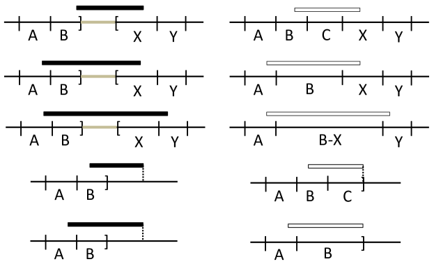
Figure 2: Illustration of the different cases in zone management, with three variations of Case 3 and two for Case 4. On the left, an incoming interval is shown in bold with the prior settings of the zones; the resulting zone configuration is shown on the right. Flexible ends of zones are shown with brackets and out-regions in grey.

This completes the specification of the zones. See Fig. 2 for illustration of the different cases.

It is clear from the definition of the zones and their endpoints that the zone collection partitions the support of the intervals seen so far. We shall assume a total order on the zones, from left to right. The following lemma is crucial for the correctness and performance guarantee of the algorithm.

Lemma 4.1.

The zone collection satisfies the following invariants:

(#)

Each zone is properly contained in an input interval, and

(*)

Each input interval properly contains at most one zone, except those intervals that when they arrive fall under Case 3 of the algorithm, which can contain two zones.

Proof.

The former invariant follows directly from the observation that in each case that a zone is created (cases 1, 3 and 4), the zone is properly contained in the input interval.

To prove the latter invariant by reductio ad absurdum, assume that there is an input sequence for which the invariant fails. Let time $t$ be the first time when the invariant does not hold on this input. Let $I_{t^{\prime\prime}}$, $t^{\prime\prime}\leq t$ be interval that contains three zones, and let these zones be (from left to right) $k_{1},k_{2}$, and $k_{3}$. Let $t^{\prime}$ be the time when zone $k_{2}$ achieved its extent as it is at time $t$.

We consider the four cases that can govern the treatment of $I_{t^{\prime}}$ by the algorithm.

In Case 1, the only zone that is created or changes its endpoint is the zone with endpoints equal to those of $I_{t^{\prime}}$. It follows that $I_{t^{\prime}}\subset I_{t^{\prime\prime}}$, which contradicts the assumption that the input intervals are proper intervals.

In Case 2, no zones are created or change their endpoints.

In Case 3, the only zone that is created or changes its endpoints is the zone $z$ that is created and includes the out-region contained in the input interval $I_{t^{\prime}}$. Furthermore, at the end of time $t^{\prime}$, zone $z$ has one adjacent zone to its right, and one adjacent zone to its left, which include the right endpoint and left endpoint or $I_{t^{\prime}}$, respectively. These zone must thus be zones $k_{1}$ and $k_{2}$. It follows that $I_{t^{\prime}}\subset I_{t^{\prime\prime}}$, a contradiction to the assumption that the input intervals are proper intervals.

Finally, consider Case 4. Without loss of generality assume that the right endpoint of $I_{t^{\prime}}$ fell in the out-region. The only zone that is created or changes its endpoint in this case is zone $z$, which has, at the end of time $t^{\prime}$, its right endpoint equal to the right endpoint of $I_{t^{\prime}}$. Furthermore, the left endpoint of $I_{t^{\prime}}$ falls in the zone adjacent to $z$ and to the left of $z$, i.e., in zone $k_{1}$. It follows again that $I_{t^{\prime}}\subset I_{t^{\prime\prime}}$, which contradicts the assumption that the input intervals are proper intervals. ∎

We next define the intervals maintained by the algorithm. For an interval $I$ and time $t$, let $\text{{bz}}(I)=\text{{bz}}_{t}(I)$ (resp. $\text{{fz}}(I)=\text{{fz}}_{t}(I)$) be the zone in which $\mathrm{left}(I)$ (resp. $\mathrm{right}(I)$) falls at time $t$. For each zone $k$, and time $t$, the algorithm keeps the endpoints of the intervals $L_{k}=\operatorname*{arg\,min}_{I\in S_{t},\text{{bz}}(I)=k,}\mathrm{left}(I)$, i.e., the one with the leftmost left endpoint in the zone, and $R_{k}=\operatorname*{arg\,max}_{I\in S_{t},\text{{fz}}(I)=k}\mathrm{right}(I)$, i.e., the one with the rightmost right endpoint in the zone. Note that $L_{k}$ (resp., $R_{k}$) will be undefined if no interval has its left (resp., right) endpoint in zone $k$.

The output of the algorithm is the maximum interval selection of the set $A=\cup_{k}\{L_{k},R_{k}\}$, obtained by, e.g., the classic left-right greedy algorithm.

We next detail how the algorithm maintains the intervals stored. When interval $I$ arrives at time $t$, we consider the four cases defined above.

If Case 1 applies, then $I$ defines a new zone $k$, and both $L_{k}$ and $R_{k}$ are permanently set to equal $I$.

If Case 2 applies, no zones change; the $L$- and $R$-intervals are updated for the zones in which the endpoints of $I$ fall. E.g., if $b(I)$ falls in zone $k$, and $b(I)<b(L_{k})$, then $L_{k}$ is updated as $I$.

If Case 3 applies, the $L$- and $R$-intervals are updated, for the zones in which the endpoints of $I$ fall. Then, a new zone is created, but all the endpoints, if any, that fall in that zone have already appeared, and thus we need only merge the information from the at most two previous flexible zones that are merged into the new zone.

If Case 4 applies, then one endpoint of $I$ falls in a zone $k$, which becomes fixed if it was not fixed before. Without loss of generality, assume it is the left endpoint of $I$ that falls in $k$. So, $L_{k}$ is updated appropriately. Then, a new zone is created; denote it $z$. If $I$ does not properly include any flexible zone, then $z$ covers $I\setminus supp(C)$, $R_{z}$ is defined to be $I$, and $L_{z}$ is undefined. If $I$ does properly include a flexible zone, denote to $k^{\prime}$, then $k^{\prime}$ is merged into $z$. $R_{z}$ is defined to be $I$, and $L_{z}$ is defined to be $L_{k^{\prime}}$.

We conclude that the algorithm can indeed maintain the intervals $L_{k}$ and $R_{k}$ for each zone $k$ as defined.

An immediate corollary of Lemma 4.1 is that the union of any five adjacent zones must properly contain an input interval. By induction, any $5t$ adjacent zones must include at least $t$ disjoint intervals. Hence, we obtain an upper bound on the space used by the algorithm by noting that for each zone $k$, only six values need to be recorded: the endpoints of $L_{k}$, of $R_{k}$ and of the zone $k$ itself. We thus have the following.

Lemma 4.2.

The number of zones is at most $5|OPT|+4$. The space used by the algorithm is at most $O(|OPT|)$.

Finally, we prove the performance guarantee of the algorithm. The following lemma captures the core of the argument. For two proper intervals $I$ and $J$, we write $I\leq J$ to denote that $\mathrm{left}(I)\leq\mathrm{left}(J)$ (and thus also $\mathrm{right}(I)\leq\mathrm{right}(J)$), and similarly $I<J$ if $\mathrm{left}(I)<\mathrm{left}(J)$.

Lemma 4.3.

Let $R\subseteq S_{t}$ be a collection of three disjoint input intervals. Then, at the end of round $t$, $A$ contains a pair of intervals of $S_{t}$ that are contained in the span of $R$.

Proof.

Let the three disjoint intervals be $O_{1}<O_{2}<O_{3}$. Our claim is that $A$ contains a pair of disjoint intervals $I,I^{\prime}\in S_{t}$, $I,I^{\prime}\subset[\mathrm{left}(O_{1}),\mathrm{right}(O_{3}))$.

Let $b_{i}=\text{{bz}}(O_{i})$ ($f_{i}=\text{{fz}}(O_{i})$) be the zone in which the left (right) endpoint of $O_{i}$ falls, for $i=1,2,3$, respectively. Clearly, $b_{1}\leq f_{1}\leq b_{2}\leq f_{2}\leq b_{3}\leq f_{3}$. We observe that $b_{1}<b_{2}<b_{3}$. Suppose, e.g., that $b_{1}=b_{2}$. Then, by Lemma 4.1(Invariant (#)), there is an interval that properly contains $O_{1}$, a contradiction. Therefore, $f_{1}<b_{3}$.

Consider $R_{f_{1}}$ and $L_{b_{3}}$, which are well-defined intervals since the right endpoint of $O_{1}$ falls in zone $f_{1}$ and the left endpoint of $O_{3}$ falls in zone $b_{3}$. By definition, $O_{1}\leq R_{f_{1}}$ and $L_{b_{3}}\leq O_{3}$, so $R_{f_{1}},L_{b_{3}}\subset[\mathrm{left}(O_{1}),\mathrm{right}(O_{3}))$. Since $f_{1}<b_{3}$, it follows that $R_{f_{1}}$ and $L_{b_{3}}$ are disjoint, establishing the claim. ∎

We conclude with the following theorem.

Theorem 4.4.

$|ALG|\geq 2|OPT|/3$.

Proof.

Let $|S|=n$, and let $O_{0},O_{1},\ldots,O_{p-1}$ be the intervals in the optimal solution in order of (left) endpoints, where $p=|OPT|$.

If $p\pmod{3}\equiv 0$, we have by Lemma 4.3 that the algorithm obtains at least two intervals within each of the segments $[\mathrm{left}(O_{3r}),\mathrm{right}(O_{3r+2)}))$, for $0\leq r\leq(p-3)/3$. Thus, we have that $|ALG|\geq 2((p-3)/3+1)=2p/3$.

If $p\pmod{3}\equiv 1$ we have by Lemma 4.3 that the algorithm obtains at least two intervals within each of the segments $[\mathrm{left}(O_{3r}),\mathrm{right}(O_{3r+2)}))$, for $0\leq r\leq(p-4)/3$. Now, if $k_{max}$ is the last zone at the end of round $n$ then $O_{p-1}\leq R_{k_{max}}$; thus the algorithm obtains an interval that intersects only $O_{p-1}$. Together we get that $|ALG|\geq 2((p-4)/3+1)+1>2p/3$.

If $p\pmod{3}\equiv 2$, we have by Lemma 4.3 that the algorithm obtains at least two intervals within each of the segments $[\mathrm{left}(O_{3r+1}),\mathrm{right}(O_{3r+3)}))$, for $0\leq r\leq(p-5)/3$. Now, if $k_{min}$ and $k_{max}$ are the first and last zones at the end of round $n$ then, $L_{k_{min}}\leq O_{0}$ and $O_{p-1}\leq R_{k_{max}}$; thus the algorithm obtains an interval that intersects only $O_{0}$ and another that intersects only $O_{p-1}$. Together we get that $|ALG|\geq 2((p-5)/3+1)+2>2p/3$. ∎

5 Lower Bounds

In this section we establish lower bounds on the approximation ratio of randomized streaming algorithms for the interval selection problem, establishing the following two theorems.

Theorem 5.1 (Lower bound for general intervals).

For every real $\epsilon>0$, integers $k_{0},n_{0}>0$, and subexponential (respectively, sublinear) function $s:\mathbb{N}\rightarrow\mathbb{N}$, there exist $k_{0}\leq k\leq c\cdot k_{0}$, where $c$ is a universal constant, $n>n_{0}$, and an interval stream $S$ such that
(1) $|S|=n$;
(2) $|\mathtt{Opt}(S)|=k$; and
(3) $\mathtt{Alg}(S)<k(1/2+\epsilon)$ for any randomized interval selection streaming algorithm $\mathtt{Alg}$ with space $s(kb)$ (resp., space $s(nb)$), where $b$ is the length of the bit strings representing the endpoints.

Theorem 5.2 (Lower bound for unit intervals).

For every real $\epsilon>0$, integers $k,n_{0}>0$, and subexponential (respectively, sublinear) function $s:\mathbb{N}\rightarrow\mathbb{N}$, there exist $n>n_{0}$, and a unit interval stream $S$ such that
(1) $|S|=n$;
(2) $|\mathtt{Opt}(S)|=k$; and
(3) $\mathtt{Alg}(S)<k(2/3+\epsilon)$ for any randomized proper interval selection streaming algorithm $\mathtt{Alg}$ with space $s(kb)$ (resp., space $s(nb)$), where $b$ is the length of the bit strings representing the endpoints.

Our lower bounds are proved by designing a random interval stream $S$ for which every deterministic algorithm performs badly on expectation; the assertion then follows by Yao’s principle. (Our construction uses half-open intervals, but this can be easily altered.) Note that under the setting used by our lower bounds, the algorithm is required to output a collection $\mathcal{C}$ of disjoint intervals, and the quality of the solution is then determined to be the cardinality of $\mathcal{C}\cap S$. In other words, the algorithm is allowed to output non-existing intervals (that is, intervals that never arrived in the input), but it will not be credited for them. This, obviously, can only increase the power of the algorithm.

The $(k,n)$-gadget.

Fix some positive integer $m$ whose role is to bound the space of the algorithm. Our lower bounds rely on the following framework, characterized by the parameters $k,n\in\mathbb{Z}_{>0}$, denoted a $(k,n)$-gadget. Consider an extensive form two-player zero-sum game played between the algorithm (MAX) and the adversary (MIN), depicted by a sequence of $k$ phases. Informally, in each phase $t$, the adversary chooses a permutation $\pi_{t}\in P_{n}$, where $P_{n}$ is the collection of all permutations on $n$ elements, and an index $i_{t}\in[n]$. The algorithm observes $\pi_{t}$ (but not $i_{t}$) and produces a memory image $M_{t}$, i.e., a bit string of length $m$. The index $i_{t}$ is handed to the algorithm after the memory image is produced. At the end of the last phase the algorithm tries to recover $\pi_{t}(i_{t})$ for $t=1,\dots,k$: it outputs some $i_{t}^{*}\in[n]$ based on the memory image $M_{t}$, index $i_{t}$, and all other memory images and indices. For each $t$ such that $i_{t}^{*}=\pi_{t}(i_{t})$, the algorithm scores a (positive) point.

More formally, the adversarial strategy is depicted by the choices of the permutations $\pi_{t}$ and the indices $i_{t}$ for $t=1,\dots,k$. We commit the adversary to make those choices uniformly at random (so, the adversary reveals its mixed strategy), namely, $\pi_{t}\in_{r}P_{n}$ and $i_{t}\in_{r}[n]$ for every $t$, where all the random choices are independent. The strategy of the algorithm is depicted by the function sequences $\{f_{t}\}_{t=1}^{k}$ and $\{g_{t}\}_{t=1}^{k}$, where

$$f_{t}:P_{n}\times\left(\{0,1\}^{m}\times[n]\right)^{t-1}\rightarrow\{0,1\}^{m}\qquad\text{and}\qquad g_{t}:\{0,1\}^{m}\times[n]\times\left(\{0,1\}^{m}\times[n]\right)^{k-1}\rightarrow[n]~{}.$$

Let $\Gamma_{0}$ be the empty string and recursively define $\Gamma_{t}=\Gamma_{t-1}\circ f_{t}\left(\pi_{t},\Gamma_{t-1}\right)\circ i_{t}$. The payoff of the algorithm is the number of $t$s, $1\leq t\leq k$, such that

$$g_{t}\left(f_{t}\left(\pi_{t},\Gamma_{t-1}\right),i_{t},\left\{f_{t^{\prime}}\left(\pi_{t^{\prime}},\Gamma_{t^{\prime}-1}\right),i_{t^{\prime}}\right\}_{t^{\prime}\neq t}\right)~{}=~{}\pi_{t}(i_{t})~{}.$$

In the language of the aforementioned informal description, the role of the function $f_{t}$ is to produce the memory image $M_{t}$ based on the permutation $\pi_{t}$ and all previous memory images and indices (whose concatenation is given by $\Gamma_{t-1}$). The role of the function $g_{t}$ is to recover $\pi_{t}(i_{t})$ based on the memory image $M_{t}$, index $i_{t}$, and all other memory images and indices.

Note that the memory images $M_{t^{\prime}}$ and indices $i_{t^{\prime}}$, $t^{\prime}\neq t$, do not contain any information on the permutation $\pi_{t}$ on top of that contained in $M_{t}$. In particular, the entropy in $\pi_{t}(i_{t})$ given $M_{t}$, $i_{t}$, and $\{M_{t^{\prime}},i_{t^{\prime}}\}_{t^{\prime}\neq t}$ is equal to the entropy in $\pi_{t}(i_{t})$ given $M_{t}$ and $i_{t}$. Therefore, it will be convenient to decompose the domain of the function $g_{t}:\{0,1\}^{m}\times[n]\times(\{0,1\}^{m}\times[n])^{k-1}\rightarrow[n]$ so that the $(\{0,1\}^{m}\times[n])^{k-1}$-part determines which function $\hat{g}_{t}:\{0,1\}^{m}\times[n]\rightarrow[n]$ is chosen, and then this function $\hat{g}_{t}$ is used to produce $i_{t}^{*}$ based on $M_{t}$ and $i_{t}$. Similarly, we decompose the domain of the function $f_{t}:P_{n}\times(\{0,1\}^{m}\times[n])^{t-1}\rightarrow\{0,1\}^{m}$ so that the $\left(\{0,1\}^{m}\times[n]\right)^{t-1}$-part determines which function $\hat{f}_{t}:P_{n}\rightarrow\{0,1\}^{m}$ is chosen, and then this function $\hat{f}_{t}$ is used to produce $M_{t}$ based on $\pi_{t}$.

We now turn to bound the expected payoff of the algorithm as a function of $k$, $m$, and $n$. The key ingredient in this context is the following lemma, which is essentially a well known fact in slightly different settings; a proof is provided in Appendix B for completeness.

Lemma 5.3.

For every real $\alpha>0$ and integer $n_{0}>0$, there exists an integer $n>n_{0}$ such that for every two functions $\hat{f}:P_{n}\rightarrow\{0,1\}^{m}$ and $\hat{g}:\{0,1\}^{m}\times[n]\rightarrow[n]$, where $m=\alpha n\log n$, we have $\mathbb{P}_{\pi\in_{r}P_{n},i\in_{r}[n]}\left(\hat{g}(\hat{f}(\pi),i)=\pi(i)\right)<2\alpha$.

Corollary 5.4.

For every real $\alpha>0$ and integers $k,n_{0}>0$, there exists an integer $n>n_{0}$ such that if $m\leq\alpha n\log n$, then the expected payoff of the algorithm player in a $(k,n)$-gadget is smaller than $2\alpha k$.

The $(n,\pi)$-stack.

We now turn to implement a $(k,n)$-gadget via a carefully designed interval stream. As a first step, we introduce the $(n,\pi)$-stack construction. Given an integer $n>0$ and a permutation $\pi\in P_{n}$, an $(n,\pi)$-stack deployed in the segment $[x,y)$, $x<y$, is a collection of $n$ intervals $J_{1},\dots,J_{n}$ satisfying:
(1) all intervals $J_{i}$ are half open;
(2) all intervals $J_{i}$ have the same length $\mathrm{right}(J_{i})-\mathrm{left}(J_{i})=\lambda n$, where $\lambda=\frac{y-x}{2n-1/2}$; and
(3) $\mathrm{left}(J_{i})=x+\lambda(i-1)+\epsilon\pi(i)$ for every $i\in[n]$, where $\epsilon=\lambda/(2n)$.
Note that this deployment ensures that $\mathrm{left}(J_{n})<\mathrm{right}(J_{1})$, hence the half open segment $[\mathrm{left}(J_{n}),\mathrm{right}(J_{1}))$ is contained in $J_{i}$ for every $i\in[n]$. Moreover, the union of the intervals in the stack does not necessarily cover the whole segment $[x,y)$; it is always contained in $[x,y)$, though. The structure of an $(n,\pi)$-stack is illustrated in Figure 3.

Figure 3: The relative locations of the intervals in an $(n,\pi)$-stack for $n=4$. The left and right endpoints of interval $J_{i}$ are located in the segments depicted by the bidirectional arrows whose length is $\lambda/2$. The exact location within this segment is determined by $\pi(i)$. In the construction of the $2$-lower bound for general intervals, the bold rectangles correspond to the segments $\sigma_{\ell}$ and $\sigma_{r}$ in which the stacks (or auxiliary intervals) identified with the left and right children, respectively, of the current node are deployed assuming that the good interval is interval $J_{2}$ (these segments do not intersect with the segments corresponding to the bidirectional arrows).

The $(k,n)$-gadget is implemented by introducing $k$ stacks, each corresponding to one phase, and some auxiliary intervals; the stack corresponding to phase $t$ is referred to as stack $t$. The permutation $\pi$ used in the construction of stack $t$ is $\pi_{t}$. The index $i_{t}$ will dictate the choice of one good interval out of the $n$ intervals in that stack. What exactly makes this interval good will be clarified soon; informally, the algorithm has no incentive to output an interval in a stack unless this interval is good.

The $k$ stacks are used both by the construction of the $2$-lower bound for general interval streams and by that of the $(3/2)$-lower bound for unit intervals. The difference between the two constructions lies in the manner in which these stacks are deployed in the real line, and in the addition of the auxiliary intervals.

A $(3/2)$-lower bound for unit intervals.

The interval stream that realizes the $(k,n)$-gadget for the $(3/2)$-lower bound for unit intervals is constructed as follows. It contains $k$ sufficiently spaced apart stacks, where the intervals in each stack are scaled to a unit length (so $\lambda=1/n$). Consider stack $t$ and suppose that it is deployed in the segment $[x,y)$, where $y=x+2-1/(2n)$. Recall that the permutation that determines the exact location of the intervals in the stack is $\pi_{t}$ and that the good interval is $J_{i_{t}}$.

After the arrival of the $n$ intervals in the stack, two more half open unit auxiliary intervals are presented:

$$L_{t}~{}=~{}\left[x+\frac{i_{t}-1}{n}-1,x+\frac{i_{t}-1}{n}\right)\qquad\text{and}\qquad R_{t}~{}=~{}\left[x+\frac{i_{t}-1/2}{n}+1,x+\frac{i_{t}-1/2}{n}+2\right)~{}.$$

In other words, the interval $L_{t}$ (respectively, $R_{t}$) is located to the left (resp., right) of the leftmost (resp., rightmost) point in which $\mathrm{left}(J_{i_{t}})$ (resp., $\mathrm{right}(J_{i_{t}})$) may be deployed. It is easy to verify that except for the good interval $J_{i_{t}}$ that does not intersect with $L_{t}$ and $R_{t}$, every interval in the stack intersects with exactly one of these two auxiliary intervals.

The best response of the algorithm would be to output the two auxiliary intervals and to try to recover the good interval $J_{i_{t}}$. (Note that the payoff guaranteed by this strategy is at least $2$ per stack, whereas any other strategy yields a payoff of at most $2$ per stack.) For that purpose, the algorithm has to recover the exact locations of the endpoints of $J_{i_{t}}$ that implicitly encode $\pi_{t}(i_{t})$. Observing that the endpoints in this construction can be represented by bit strings of length $\log(n)+\log(k)$, Theorem 5.2 follows by Corollary 5.4.

A $2$-lower bound for general intervals.

The interval stream that realizes the $(k,n)$-gadget for the $2$-lower bound for general intervals is constructed as follows. Assume that $k=2^{\kappa}-1$ for some positive integer $\kappa$ and consider a perfect binary tree $T$ of depth $\kappa$. The $k$ stacks are identified with the internal nodes of $T$ so that stack $t$ precedes stack $t+1$ in a pre-order traversal of $T$. (In other words, if stack $t$ is identified with node $u$ and stack $t^{\prime}$ is identified with a child of $u$, then $t<t^{\prime}$.) In addition to the intervals in the stacks, we also introduce $2^{\kappa}=k+1$ auxiliary intervals which are identified with the leaves of $T$; these auxiliary intervals arrive last in the stream. We say that an interval $J$ is assigned to node $u\in T$ if $J$ belongs to the stack identified with $u$ or if $u$ is a leaf and $J$ is the auxiliary interval identified with it.

The deployment of the stacks and the auxiliary intervals in $\mathbb{R}$ is performed as follows. Stack $1$ (identified with $T$’s root) is deployed in $[0,1)$. Given the deployment of stack $t$ identified with internal node $u\in T$ in the segment $[x,y)$, we deploy the stacks identified with the left and right children of $u$ in the segments

$$\sigma_{\ell}~{}=~{}\left[x+\lambda(i_{t}-3/2),x+\lambda(i_{t}-1)\right)\qquad\text{and}\qquad\sigma_{r}~{}=~{}\left[x+\lambda(i_{t}+n-1/2),x+\lambda(i_{t}+n)\right)~{},$$

respectively, where recall that $\lambda=\frac{y-x}{2n-1/2}$. If the children of $u$ are leaves in $T$, then we deploy auxiliary intervals in those two segments instead of stacks, that is, one auxiliary interval in $\sigma_{\ell}$ and one in $\sigma_{r}$. Refer to Figure 3 for illustration.

The key observation regarding the choice of $\sigma_{\ell}$ and $\sigma_{r}$ is that

$$\mathrm{left}(J_{i_{t}-1})\leq\mathrm{left}(\sigma_{\ell})<\mathrm{right}(\sigma_{\ell})\leq\mathrm{left}(J_{i_{t}})\quad\text{and}$$

$$\mathrm{right}(J_{i_{t}})\leq\mathrm{left}(\sigma_{r})<\mathrm{right}(\sigma_{r})\leq\mathrm{right}(J_{i_{t}+1})\,.$$

In particular, this implies that: (1) the good interval in the stack identified with node $u\in T$ does not intersect with any interval assigned to a descendant of $u$ in $T$; and (2) a non-good interval in the stack identified with node $u\in T$ contains every interval assigned to a descendant of either the left child of $u$ or the right child of $u$ in $T$.

Since the $k+1$ auxiliary intervals are non-intersecting and arrive last in the stream, they can be included in the output of the algorithm without requiring any additional space (on top of that dedicated to their representation). Moreover, an auxiliary interval intersects with at most one interval in any valid solution, hence it is a dominant strategy on behalf of the algorithm to output all the auxiliary intervals. Therefore, the best response of the algorithm can include an interval $J_{i}$ of stack $t$, $1\leq t\leq k$, in the output only if it is the good interval of that stack, namely, $i=i_{t}$.

By definition, in order to include interval $J_{i_{t}}$ of stack $t$ in the output, the algorithm must hold the exact locations of its endpoints. The construction of stack $t$ based on permutation $\pi_{t}$ implies that the exact locations of interval $J_{i_{t}}$’s endpoints encode the value of $\pi_{t}(i_{t})$. Observing that the endpoints in this construction can be represented by bit strings of length $\log(n)\cdot\log(k)$, Theorem 5.1 follows by Corollary 5.4.

6 Multiple-Pass Algorithms

We extend now the streaming algorithms to use multiple passes through the data. First, some notation. For an interval $I$, let $next(I)$ be the interval in the input that ends earliest among those that start after $I$ ends, and let $prev(I)$ be the interval that starts latest among those that finish before $I$ starts. We use the notation $next^{i}(I)$ defined recursively as $I$ when $i=0$ and as $next(next^{i-1}(I))$ for $i>0$, and define $prev^{i}(I)$ similarly. Observe that if $I$ is available before a pass, then a streaming algorithm can easily compute $next(I)$ and $prev(I)$ by the end of the pass, while maintaining $O(1)$ intervals in the memory at all times.

The multi-pass algorithm runs as follows. The first pass consists of the earlier one-pass algorithm, either as the algorithm of Sec. 3 for general intervals, or the algorithm of Sec. 4 for proper intervals. The result of this pass is the set $A$, whichever base algorithm is used. Let $N_{0}=P_{0}=A$. In round $p>1$, the algorithm inductively computes $N_{p-1}=\{next(I):I\in N_{p-2}\}$ and $P_{p-1}=\{prev(I):I\in P_{p-2}\}$. Let $A_{p}=\cup_{i\geq 0}^{p-1}(N_{i}\cup P_{i})=\{next^{i}(I),prev^{i}(I):I\in A,0\leq i\leq p-1\}$ denote the combined set of intervals stored after pass $p$. When requested, the algorithm produces as output the maximum interval selection in $A_{p}$. This completes the specification of the algorithm.

We first observe that $|A_{p}|\leq(2p-1)A$, hence the space used in phase $p$ is at most $2p-1$ times larger than the length of the bit string representing $A$.

Define the span of a set $R$ of intervals to be the segment with endpoints being the leftmost left endpoint of the intervals in $R$, and the rightmost right endpoint of the intervals in $R$.

Lemma 6.1.

Given an input of general intervals, the set $A$ computed by the algorithm $\mathtt{Alg}$ of Sec. 3 satisfies the following property: for any pair of disjoint intervals $I_{1}$ and $I_{2}$ in the input, $A$ contains an interval within the span of $\{I_{1},I_{2}\}$ (given by $[\mathrm{left}(I_{1}),\mathrm{right}(I_{2}))$, assuming $I_{1}<I_{2}$).

The following lemmas apply both to general or proper intervals. An interval is said to be end-simplicial with respect to a set of intervals $X$, if it contains either the leftmost right endpoint or the rightmost left endpoint of its connected component with respect to $X$.

Lemma 6.2.

The set $A$ contains all the end-simplicial intervals with respect to $S$.

Proof.

Regarding general intervals, recall from Proposition 3.1 that virtual intervals in $\mathtt{Alg}$ are formed by the intersection of two intervals in the input. Thus, if $I$ is end-simplicial with respect to $S$, it contains no virtual interval, and certainly no actual intervals. Hence, $I$ is admitted to $A$ and never rejected. For proper intervals, an end simplicial interval on the left (right) will always represent $R_{k}$ ($L_{k}$) for its finishing (beginning) zone $k$. Thus, it is contained in $A$. ∎

Lemma 6.3.

let $I$ be an interval in $A_{p}$ and let $s\leq p-1$. Let $R\subseteq S$, s.t. $I\in R$ be a set of $s+1$ disjoint intervals. Then, $A_{p}$ contains a set of $s+1$ intervals within the span of $R$.

Proof.

Suppose $R$ contains intervals $I,I_{1},I_{2},\ldots,I_{s}$ , s.t. $I_{1}<I_{2}\ldots I_{j}<I<I_{j+1}<\ldots<I_{s}$. By definition, the intervals $next^{i}(I)$, $0\leq i\leq s-j$, are disjoint and contained in $A_{s+1}$ and thus also in $A_{p}$. Also, by induction, $next^{i}(I)\leq I_{i}$, for $i=1,\ldots,s-j$, and thus they fall within the span of $R$. A similar claim holds for the intervals $prev^{i}(I)$, $0\leq i\leq j$ ∎

Lemma 6.4.

Consider any set $R$ of $m$ disjoint intervals in $S$, where $m=2p$ for general intervals and $m=2p+1$ for proper intervals. Then, $A_{p}$ contains $m-1$ intervals within the span of $R$.

Proof.

Follows from Lemma 6.3, along with Lemma 6.1 (resp. Lemma 4.3) for general (resp. proper) intervals. ∎

Theorem 6.5.

The multi-pass algorithm finds a solution for the interval selection problem on general intervals that is a $1+\frac{1}{2p-1}$-approximation, at the end of each pass $p$. On proper intervals it finds a $1+\frac{1}{2p}$-approximation. The space used by the algorithm is $O(p)$ times the size of the output.

Proof.

Define $m=2p$ for general intervals and $m=2p+1$ for proper intervals. Consider an optimal interval selection with intervals $I_{1},\ldots,I_{|OPT|}$, where $\alpha=|OPT|$. Let $r=\alpha\bmod m$, and $q=\lfloor\alpha/m\rfloor$. Also let $t=\lceil r/2\rceil$ and $t^{\prime}=\lfloor r/2\rfloor$. For each $R_{i}=\{I_{t+1+im},\ldots,I_{t+(i+1)m}\}$, where $i=0\ldots,q-1$, it holds by Lemma 6.4 that $A_{p}$ contains $m-1$ intervals within the span of $R_{i}$. By Lemmas 6.2 and 6.3, $A_{p}$ also contains $t$ disjoint intervals within the span of $[\mathrm{left}(S),\mathrm{right}(I_{t})]$ and $t^{\prime}$ disjoint intervals within the span of $[\mathrm{left}(I_{m-t^{\prime}+1}),\mathrm{right}(S)]$. Hence, $A_{p}$ contains at least $q(m-1)+t+t^{\prime}=\alpha-q\geq\alpha(m-1)/m$ disjoint intervals. ∎

7 Online Algorithm

In this section we briefly show how to use the streaming algorithm presented in Sec. 3 to derive a randomized preemptive online interval selection algorithm. Our algorithm is $6$-competitive and on top of maintaining at any time the set of currently accepted intervals $A^{*}$, its only additional memory is an interval set of cardinality linear in the size of the current optimum. We thus answer an open question of Adler and Azar [1] about the space complexity of randomized preemptive online algorithms for our problem.

Recall that our streaming algorithm maintains a set $A$ of intervals. With respect to that set, our algorithm is a deterministic preemptive online algorithm, adding an interval to $A$ only when that interval arrives, and possibly preempting it later. By Corollary 3.7, the cardinality of the set $A$ is at least half the cardinality of the optimal solution of the input seen so far. Moreover, combining Lemma 3.4(P6) and Lemma 3.4(P7), we conclude that every interval added to $A$ intersects with at most $2$ previous intervals in $A$. Therefore, $A$ is online $3$-colorable: upon addition into $A$, each interval can be assigned one of three colors, such that intersecting intervals always have different colors.

Our preemptive algorithm is now simple. We initially pick a random color $c$ in $\{1,2,3\}$. We then run the streaming algorithm on each received interval $I$, adding $I$ to $A$, and preempting intervals from $A$ as does the streaming algorithm. If $I$ is added to $A$ we assign it a valid color from $\{1,2,3\}$ in a first-fit manner. Our solution $ALG$ consists of every interval $J$ in $A$ whose color is $c$. Clearly, $E[|ALG|]=|A|/3\geq|OPT|/6$, that is, the algorithm is $6$-competitive.

Acknowledgments

We thank Jaikumar Radhakrishnan and Oded Regev for helpful discussions.

APPENDIX

Appendix A Lifting the Distinct Endpoints Assumption

Recall that our analysis assumes that all the intervals in the stream $S$ are closed and that their endpoints are distinct. In this section we show that these assumptions can be lifted. A quick glance at our algorithm reveals that it is essentially comparison-based, namely, it can be implemented via a comparison oracle $\mathcal{C}:\mathbb{R}^{2}\rightarrow\{-1,0,+1\}$ without accessing the interval’s endpoints in any other way; given two endpoints $p,q$ of intervals in $S$, the comparison oracle returns

$$\mathcal{C}(p,q)~{}=~{}\left\{\begin{array}[]{ll}-1&\text{ if }p<q\\ 0&\text{ if }p=q\\ +1&\text{ if }p>q~{}.\end{array}\right.$$

The assumption that all endpoints are distinct means that the algorithm and its analysis rely on a comparison oracle $\mathcal{C}^{\prime}:\mathbb{R}^{2}\rightarrow\{-1,0,+1\}$ with the additional guarantee that $\mathcal{C}^{\prime}(p,q)\neq 0$ whenever $p\neq q$. We shall refer to such a comparison oracle $\mathcal{C}^{\prime}$ as a distinct-endpoints comparison oracle.

We show that for every stream $S$ of intervals (the endpoints of these intervals may be arbitrarily open or closed) associated with a comparison oracle $\mathcal{C}$, there exists a distinct-endpoints comparison oracle $\mathcal{C}^{\prime}$ such that for every two intervals $I,J\in S$, the closure of $I$ and the closure of $J$ intersect under $\mathcal{C}^{\prime}$ if and only if $I$ and $J$ intersect under $\mathcal{C}$. Moreover, given an access to the comparison oracle $\mathcal{C}$, the distinct-endpoints comparison oracle $\mathcal{C}^{\prime}$ can be implemented under our streaming model’s space requirements.

The distinct-endpoints comparison oracle $\mathcal{C}^{\prime}$ is designed as follows. Consider an endpoint $p$ of an interval $I\in S$ and an endpoint $q$ of an interval $J\in S$, $I\neq J$. If $\mathcal{C}(p,q)\neq 0$, then we set $\mathcal{C}^{\prime}(p,q)=\mathcal{C}(p,q)$, so assume hereafter that $\mathcal{C}(p,q)=0$. Consider first the case in which $p$ is a right endpoint and $q$ is a left endpoint (the converse case is analogous). If at least one of the endpoints is open, then set $\mathcal{C}^{\prime}(p,q)=-1$; otherwise (both endpoints are closed), set $\mathcal{C}^{\prime}(p,q)=+1$.

Now, consider the case in which both $p$ and $q$ are left endpoints (the converse case is analogous). If $p$ is open and $q$ is closed, then set $\mathcal{C}^{\prime}(p,q)=+1$; if $p$ is closed and $q$ is open, then set $\mathcal{C}^{\prime}(p,q)=-1$; if both $p$ and $q$ are open or both are closed, then we set

$$\mathcal{C}^{\prime}(p,q)~{}=~{}\left\{\begin{array}[]{ll}+1&\text{ if $I$ (the interval of $p$) arrived before $J$ (the interval of $J$)}\\ -1&\text{ if $I$ (the interval of $p$) arrived after $J$ (the interval of $J$).}\end{array}\right.$$

It is easy to verify that the closures of every two intervals intersect under $\mathcal{C}^{\prime}$ if and only if the intervals themselves intersect under $\mathcal{C}$. Therefore, it remains to show that $\mathcal{C}^{\prime}$ can be implemented in the streaming model. Apart from an access to the original comparison oracle $\mathcal{C}$, the implementation of $\mathcal{C}^{\prime}(p,q)$ is based on: (1) knowing for each endpoint whether it is a left endpoint or a right endpoint; (2) knowing for each endpoint whether it is open or closed; and (3) knowing the order of arrival of intervals that share a left (respectively, right) endpoint. The first two requirements are clearly satisfied by the information provided in the input. For the third requirement, we note that if two intervals share a left (resp., right) endpoint $p$, then they must intersect. Thus, Lemma 3.4(P5) and Lemma 3.4(P6) guarantee that at any given time, our algorithm maintains $O(1)$ intervals that have $p$ as their left (resp., right) endpoint. A data structure that tracks the arrival order of these intervals can therefore be implemented with $O(1)$ additional bits per interval.

Appendix B Proof of Lemma 5.3

Let $n$ be sufficiently large so that $n(1+\log(e))\leq\alpha n\log(n)$. Suppose toward a contradiction that there exist two functions $\hat{f}:P_{n}\rightarrow\{0,1\}^{m}$ and $\hat{g}:\{0,1\}^{m}\times[n]\rightarrow[n]$ such that $\mathbb{P}(\hat{g}(\hat{f}(\pi),i)=\pi(i))\geq 2\alpha$. We shall use these functions to construct a uniquely decodable coding scheme $s:P_{n}\rightarrow\{0,1\}^{*}$ so that $\mathbb{E}_{\pi\in_{r}P_{n}}[|s(\pi)|]<\log(n!)$. This contradicts Shannon’s source coding theorem as the entropy of choosing $\pi$ uniformly at random from $P_{n}$ is $\log(n!)$.

In order to construct the coding scheme, we first define the vector $v_{\pi}\in\{0,1\}^{n}$ for every $\pi\in P_{n}$ by setting $v_{\pi}(i)=1$ if $\hat{g}(\hat{f}(\pi),i)=\pi(i)$; and $v_{\pi}(i)=0$ otherwise. Let $W_{\pi}=\{i\in[n]\mid v_{\pi}(i)=0\}$. The coding scheme $s$ is now defined by setting the codeword of each $\pi\in P_{n}$ to be

$$s(\pi)~{}=~{}v_{\pi}\circ\hat{f}(\pi)\bigcirc_{i\in W_{\pi}}\pi(i)~{},$$

where $\bigcirc_{i\in W_{\pi}}\pi(i)$ denotes a concatenation of the standard binary representations of $\pi(i)$ for all $i\in W_{\pi}$ listed in increasing order of the index $i$.

We first argue that $s$ is indeed a uniquely decodable code. To that end, notice that for every $\pi\in P_{n}$ and for every $i\in[n]$, we can extract the value of $\pi(i)$ from $s(\pi)$ as follows:
(1) Check in $v_{\pi}$ if the correct value of $\pi(i)$ can be extracted from $\hat{f}(\pi)$, that is, if $v_{\pi}(i)=1$.
(2) If it can ($v_{\pi}(i)=1$), then $\pi(i)$ is extracted by computing $\hat{g}(\hat{f}(\pi),i)$ (recall that $\hat{f}(\pi)$ is found in the second segment of $s(\pi)$).
(3) Otherwise ($v_{\pi}(i)=0$), $\pi(i)$ is extracted from the third segment of $s(\pi)$.
Moreover, the coding scheme $s$ is prefix-free (and hence uniquely decodable) since $v_{\pi}=v_{\pi^{\prime}}$ implies that $|s(\pi)|=|s(\pi^{\prime})|$ for every two permutations $\pi,\pi^{\prime}\in P_{n}$. Thus, if the codewords $s(\pi)$ and $s(\pi^{\prime})$ agree on the first $n$ bits, then they must have the same length, which means that $s(\pi)$ cannot be a proper prefix of $s(\pi^{\prime})$.

It remains to show that $\mathbb{E}_{\pi\in_{r}P_{n}}[|s(\pi)|]<\log(n!)$. By definition, $|s(\pi)|=n+m+\log(n)\cdot|W_{\pi}|$ for every $\pi\in P_{n}$, so

$$\mathbb{E}_{\pi\in_{r}P_{n}}[|s(\pi)|]~{}=~{}n+m+\log(n)\cdot\mathbb{E}_{\pi\in_{r}P_{n}}[|W_{\pi}|]~{}.$$

The assumption that $\mathbb{P}_{\pi\in_{r}P_{n},i\in_{r}[n]}(\hat{g}(\hat{f}(\pi),i)=\pi(i))\geq 2\alpha$ implies that $\mathbb{P}_{\pi\in_{r}P_{n},i\in_{r}[n]}(i\in W_{\pi})\leq 1-2\alpha$, hence $\mathbb{E}_{\pi\in_{r}P_{n}}[|W_{\pi}|]\leq(1-2\alpha)n$. Plugging $m=\alpha n\log(n)$, we conclude that

$$\mathbb{E}_{\pi\in_{r}P_{n}}[|s(\pi)|]~{}\leq~{}n+(1-\alpha)n\log(n)~{}.$$

By the choice of $n$ (satisfying $n(1+\log(e))\leq\alpha n\log(n)$), we derive the desired inequality since $\log(n!)>n\log(n)-n\log(e)$. The assertion follows.

References

- [1] R. Adler and Y. Azar. Beating the logarithmic lower bound: Randomized preemptive disjoint paths and call control algorithms. J. Scheduling, 6(2):113–129, 2003.
- [2] P. K. Agarwal and R. Sharathkumar. Streaming algorithms for extent problems in high dimensions. In SODA, pages 1481–1489, 2010.
- [3] K. Ahn and S. Guha. Graph sparsification in the semi-streaming model. In ICALP, pages 328–338, 2009.
- [4] N. Alon, Y. Matias, and M. Szegedy. The space complexity of approximating the frequency moments. J. Comput. Syst. Sci., 58(1):137–147, 1999.
- [5] B. Awerbuch, Y. Bartal, A. Fiat, and A. Rosén. Competitive non-preemptive call control. In SODA, pages 312–320, 1994.
- [6] U. T. Bachmann, M. M. Halldórsson, and H. Shachnai. Online scheduling intervals and -intervals. In SWAT, 2010.
- [7] S. Cabello and P. Pérez-Lantero. Interval Selection in the Streaming Model. ArXiv e-prints, Jan. 2015.
- [8] R. Canetti and S. Irani. Bounding the power of preemption in randomized scheduling. SIAM J. Comput., 27(4):993–1015, 1998.
- [9] T. H. Cormen, C. E. Leiserson, R. L. Rivest, and C. Stein. Introduction to Algorithms. MIT Press and McGraw-Hill, 3rd edition, 2009.
- [10] Y. Emek, M. Halldórsson, and A. Rosén. Space-constrained interval selection. In ICALP, pages 302–313, 2012.
- [11] L. Epstein and A. Levin. Improved randomized results for the interval selection problem. Theor. Comput. Sci., 411(34-36):3129–3135, 2010.
- [12] L. Epstein, A. Levin, J. Mestre, and D. Segev. Improved approximation guarantees for weighted matching in the semi-streaming model. In STACS, pages 347–358, 2010.
- [13] J. Feigenbaum, S. Kannan, A. McGregor, S. Suri, and J. Zhang. On graph problems in a semi-streaming model. Theor. Comput. Sci., 348:207–216, December 2005.
- [14] J. Feigenbaum, S. Kannan, A. McGregor, S. Suri, and J. Zhang. Graph distances in the data-stream model. SIAM J. Comput., 38(5):1709–1727, 2008.
- [15] S. Fung, C. Poon, and F. Zheng. Improved randomized online scheduling of unit length intervals and jobs. In WAOA, 2008.
- [16] F. Gavril. Algorithms for minimum coloring, maximum clique, minimum covering by cliques, and maximum independent set of a chordal graph. SIAM J. Comput., 1(2):180–187, 1972.
- [17] B. V. Halldórsson, M. M. Halldórsson, E. Losievskaja, and M. Szegedy. Streaming algorithms for independent sets. In ICALP, pages 641–652, 2010.
- [18] M. R. Henzinger, P. Raghavan, and S. Rajagopalan. Computing on data streams. In AMS-DIMACS series, special issue on computing on very large datasets. 1998.
- [19] J. Kleinberg and E. Tardos. Algorithm Design. Addison Wesley, 2005.
- [20] S. Leonardi, A. Marchetti-Spaccamela, A. Presciutti, and A. Rosén. On-line randomized call control revisited. SIAM J. Comput., 31(1):86–112, 2001.
- [21] R. J. Lipton and A. Tomkins. Online interval scheduling. In SODA, pages 302–311, 1994.
- [22] A. McGregor. Finding graph matchings in data streams. In APPROX-RANDOM, pages 170–181, 2005.
- [23] J. I. Munro and M. Paterson. Selection and sorting with limited storage. Theor. Comput. Sci., 12:315–323, 1980.
- [24] S. Muthukrishnan. Data streams: Algorithms and applications. Foundations and Trends in Theoretical Computer Science, 1(2), 2005.
- [25] G. J. Woeginger. On-line scheduling of jobs with fixed start and end times. Theor. Comput. Sci., 130(1):5–16, 1994.