Gibbs-non-Gibbs transitions via large deviations: computable examples

Abstract

We give new and explicitly computable examples of Gibbs-non-Gibbs transitions of mean-field type, using the large deviation approach introduced in [4]. These examples include Brownian motion with small variance and related diffusion processes, such as the Ornstein-Uhlenbeck process, as well as birth and death processes. We show for a large class of initial measures and diffusive dynamics both short-time conservation of Gibbsianness and dynamical Gibbs-non-Gibbs transitions.

1 Introduction

Starting from [3] dynamical Gibbs-non-Gibbs transitions have been considered by several authors, see e.g. [2], [10], [6]. In these studies, one considers lattice spin systems started from a Gibbs measure $\mu$ at time zero and evolves it according to a Markovian dynamics (e.g. Glauber dynamics) with stationary Gibbs measure $\nu\not=\mu$. The question is then whether $\mu_{t}$, the time-evolved measure at time $t>0$ is a Gibbs measure. Typically this is the case for short times, whereas for longer times, there can be transitions from Gibbs to non-Gibbs (loss) and back from non-Gibbs to Gibbs (recovery). The notion of a “bad configuration”, i.e., a point of essential discontinuity of the conditional probabilities of the measure $\mu_{t}$ is crucial here. Such a configuration $\eta_{spec}$ is typically identified by looking at the joint distribution of the system at time $0$ and at time $t$. If conditioned on $\eta_{spec}$ the system at time zero has a phase transition, then typically $\eta_{spec}$ is a bad configuration.

In the context of mean-field models, the authors in [9] started with an analysis of the most probable trajectories (in the sense of large deviations) of a system conditioned to arrive at time $T$ at a given configuration. The setting of [9] is the Curie-Weiss model subjected to a spin-flip dynamics. A Gibbs-non-Gibbs transition is in this context rephrased as a phenomenon of “competing histories”, i.e., for special terminal conditions $x_{spec}$ and times $T$ not too small, multiple trajectories can minimize the rate function, and these trajectories can be selected by suitably approximating $x_{spec}$. These special conditionings leading to multiple histories are the analogue of “bad configurations” (essential points of discontinuity of conditional probabilities of the measure at time $t$) in the Gibbs-non-Gibbs transition scenario. This “trajectory large deviation approach” has then been studied in more generality, including the lattice case, in [4].

In this paper, we apply the trajectory large deviation approach in several examples, both for diffusion processes and for birth and death processes. This leads to new and explicitly computable Gibbs-non-Gibbs transitions of mean field type. For processes of diffusion type, we first treat an explicit example for the rate function of the initial measure, and as dynamics Brownian motion with small variance or Ornstein-Uhlenbeck process. In all cases, we obtain the explicit form of the conditioned trajectories, and explicit formulas for the bad configuration and the time at which it becomes bad. In the case of general Markovian diffusion processes in a symmetric potential landscape, we show under reasonable conditions short-time Gibbsianness as well as appearance of bad configurations at large times. Next, we treat the case of continuous-time random walk with small increments, as arises e.g. naturally in the context of (properly rescaled) population dynamics. In that case, the Euler-Lagrange trajectories can be explicitly computed for some particular choices of the “birth and death” rates. Constant birth and death rates are the analogue of the Brownian motion case, whereas linear birth and death rates are the analogue of the Ornstein-Uhlenbeck process, but in that case the cost of optimal trajectories becomes a much more complicated expression.

Our paper is organized as follows. In section 2 we introduce some elements or the Feng-Kurtz formalism, and define the notion of bad configurations in the present setting. In section 3 we treat diffusion processes with small variance, with an explicit form for the initial rate function. In section 3.3 we treat the case of Brownian motion dynamics with different cases for the rate function of the initial measure. Finally, in section 5, we treat one-dimensional random walks with small increments, such as rescaled birth and death processes.

2 The Feng-Kurtz scheme, Euler-Lagrange trajectories, bad configurations

We study Markov processes $\{X^{n}_{t}:0\leq t\leq T\}$ taking values in $\mathbb{R}^{d}$, parametrized by a natural number $n$. This parameter tunes the “amount of noise” in the process, i.e., as $n\to\infty$, the process becomes deterministic, and the measure on trajectories satisfies the large deviation principle with rate $n$ and with a rate function of the form

$${\mathscr{I}}(\gamma)=\int_{0}^{T}L(\gamma_{s},\dot{\gamma}_{s})ds$$ (1)

This means more precisely that

$$\mathbb{P}\left(\{X^{n}_{t}:0\leq t\leq T\}\approx\gamma\right)\approx\exp\left(-n{\mathscr{I}}(\gamma)\right)$$ (2)

to be interpreted in the usual sense of the large deviation principle with a suitable topology on the set of trajectories. The form (1) naturally follows from the Markov property.

Notice that the form of the rate function does not depend on the choice of this topology. So one usually starts with the weakest topology, i.e., the product topology, and then, if possible, strengthens the topology by showing exponential tightness. See [1] for an illustration of this strategy in the context of theorems like Mogulskii’s theorem.

Since in this paper we are only interested in finding out optimal trajectories, i.e., minimizers of the rate function over a set of trajectories with prescribed terminal condition and open-end condition, we will not have to worry about the strongest topology in which the large deviation principle (2) holds, but we are rather after (as explicit as possible) solutions of Euler-Lagrange problems associated to the rate function.

In [8] a scheme is given to compute the “Lagrangian” $L$, see also [4] for an illustration of this scheme in the large-deviation view on Gibbs-non-Gibbs transitions. First one computes the “Hamiltonian”

$${\mathscr{H}}(p,x)=\lim_{n\to\infty}\frac{1}{n}e^{-n\langle p,x\rangle}{\mathscr{L}}_{n}e^{n\langle p,x\rangle}$$ (3)

where ${\mathscr{L}}_{n}$ is the generator of the process $\{X^{n}_{t}:0\leq t\leq T\}$ (working on the $x$-variable, where $p\in\mathbb{R}^{d}$ is the “momentum” and where $<.,.>$ denotes inner product. . Under regularity conditions on ${\mathscr{H}}(p,x)$ (e.g. strict convexity), the associated Lagrangian is then given by the Legendre transform

$$L(x,v)=\sup_{p\in\mathbb{R}^{d}}\left(<v,p>-{\mathscr{H}}(x,p)\right),$$ (4)

As an example, consider

$$X^{n}_{t}=n^{-1/2}B_{t}$$

with generator

$${\mathscr{L}}_{n}=\frac{1}{2n}\Delta$$

then we have

$${\mathscr{H}}(x,p)=\frac{p^{2}}{2}$$

and associated Lagrangian

$$L(x,v)=\frac{v^{2}}{2}$$

which produces the rate function of the well-known Schilder’s theorem

$$\mathbb{P}\left(\{X^{n}_{t}:0\leq t\leq T\}\approx\gamma\right)\approx\exp\left(-\frac{n}{2}\int_{0}^{T}\dot{\gamma}_{s}^{2}ds\right)$$

To proceed, we also want the initial point of our process to have some fluctuations. More precisely, we need for the starting point of our process an initial measure $\mu_{n}$ (depending on $n$) on $\mathbb{R}^{d}$, satisfying the large deviation principle with rate $n$ and rate function $i(x)$, i.e., in the sense of large deviations, we assume

$$\mathbb{P}\left(X^{n}_{0}\in A\right)=\mu_{n}(A)\approx\exp(-n\inf_{x\in A}i(x))$$ (5)

We call the triple $(\{X^{n}_{t}:0\leq t\leq T\},L,i)$ a stochastic system with small noise.

We continue now with the definition of a bad configuration in this framework. This is motivated by the definition of a bad configuration in the context of mean-field models [9], and can be viewed as the large-deviation rephrasing of “a phase transition at time zero conditioned on a special configuration at time $T$”.

DEFINITION 2.1.

Let $(\{X^{n}_{t}:0\leq t\leq T\},L,i)$ be a stochastic system with small noise. We say that a point $b\in\mathbb{R}^{d}$ is bad at time $T$ if the following two conditions hold.

1. Conditional on $X^{n}_{T}=b$, $X^{n}_{0}$ does not converge (as $n\to\infty$) to a pointmass in distribution.

2. There exist two sequences $b^{+}_{k}\to b$, $b^{-}_{k}\to b$ and $\delta>0$ such that the variational distance between the distribution $\mu(0,T;b^{+}_{k})$ of $X^{n}_{0}|X^{n}_{T}=b^{+}_{k}$ and the distribution $\mu(0,T;b^{-}_{k})$ of $X^{n}_{0}|X^{n}_{T}=b^{-}_{k}$ is at least $\delta$ for $k$ large enough.

The simplest example which follows also the most common scenario is where the distribution of $X^{n}_{0}|X^{n}_{T}=b$ converges to $\frac{1}{2}(\delta_{-a}+\delta_{a})$ and for $c>b$ $X^{n}_{0}|X^{n}_{T}=c$ converges to $\delta_{\alpha(c)}$ where $\alpha(c)\to a$ as $c\downarrow b$, whereas for $c<b$ $X^{n}_{0}|X^{n}_{T}=c$ converges to $\delta_{\alpha^{\prime}(c)}$ where $\alpha^{\prime}(c)\to-a$ as $c\uparrow b$. This means that conditioned to be at time $T$ at location $b$, the process has two “favourite” intial spots, which can be “selected” by approaching $b$ from the right or from the left.

This is the analogue of a phase transition, where the phases can be selected by appropriately approximating the bad configuration, see [3].

3 Diffusion processes with small variance conditioned on the future

In this section we present examples where $X^{n}_{t}$ is a diffusion process. We show also how from the large deviation approach we gain a new understanding of “short-time Gibbsianness” for a general class of drifts of the diffusion, or initial rate functions.

3.1 Brownian motion

To start with, we consider Brownian motion with small variance $\frac{1}{n}$ starting from an initial distribution satisfying the large deviation principle (with rate $n$) with a non-convex rate function having two mimina at locations $-a,a$, with $a>0$. More precisely, we consider the process

$$X^{n}_{t}=\frac{1}{\sqrt{n}}B_{t}$$ (6)

starting from an initial distribution $\mu_{n}$ such that, informally written,

$$\mathbb{P}\left(X^{n}_{0}\in dx\right)=\mu_{n}(dx)\approx e^{-ni(x)}dx$$ (7)

For $i$ we make the explicit choice:

$$i(x)=(x^{2}-a^{2})^{2}$$ (8)

i.e., a non-convex function non-negative with zeros at $-a,a$ and maximum at $x=0$ ($i(x)$ with $a=2$ is plotted in Figure 1).

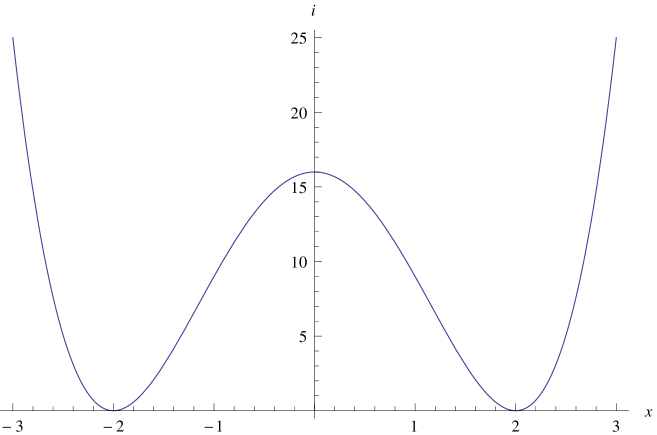
Figure 1: $i(x)=(x^{2}-a^{2})^{2}$ with $a=2$

This specific choice is for the sake of explicit analytic computability but many results are true for a general class of rate functions that have a similar graph with two zeros located at $-a,a$ and a maximum at zero.

More formally, we require that the sequence of initial probability measures $\{\mu_{n},n\in\mathbb{N}\}$ satisfies the large deviation principle with rate function $i$ given by (8). Such rate functions arise naturally in the context of mean-field models with continuous spins and spin-Hamiltonian depending on the magnetization.

We are then interested in the most probable trajectory $\gamma$ with initial point distributed according to $\mu_{n}$ and final point $\gamma_{T}=0$. More precisely, by application of Schilder’s theorem, the trajectory $\{X^{n}_{t}:0\leq t\leq T\}$ satisfies the LDP with rate function

$${\mathscr{I}}(\gamma)=\frac{1}{2}\int_{0}^{T}\dot{\gamma}_{s}^{2}ds+i(\gamma_{0})$$ (9)

The optimal trajectory we are looking for is hence

$$\arg\min\{{\mathscr{I}}(\gamma):\gamma(T)=0\}$$

The Euler-Lagrange trajectories (extrema of the cost $\frac{1}{2}\int_{0}^{T}\dot{\gamma}_{s}^{2}ds$ corresponding to ${\mathscr{I}}(\gamma)$) are linear in $t$:

$$\gamma_{t}=A+Bt$$

By the terminal condition $B=-A/T$.

The cost ${\mathscr{I}}(\gamma)$ of this trajectory can then be rewritten as a function of the starting point $\gamma_{0}=A$:

$${\mathscr{E}}_{0,T}(A):={\mathscr{I}}(\gamma)=A^{4}-2a^{2}A^{2}+a^{4}+\frac{1}{2}(-A/T)^{2}T=A^{4}+\alpha(a,T)A^{2}+a^{4}$$ (10)

with

$$\alpha(a,T)=\left(\frac{1}{2T}-2a^{2}\right)$$ (11)

The behavior of this cost depends on the sign of $\alpha$. If $\alpha\geq 0$, then there is a unique minimum at $A=0$, this case corresponds to

$$T\leq\frac{1}{4a^{2}}:=T_{crit}$$

If $\alpha<0$ then there are two mimima $A=A_{\pm}$ given by

$$A_{\pm}=\pm\sqrt{-\alpha(a,T)/2}=\pm\sqrt{a^{2}-(4T)^{-1}}$$ (12)

We thus conclude that, as $n\to\infty$, the starting point is most probably $0$ for small $T$ and most (and equally) probably $A_{\pm}$ for large $T$, which converges to $\pm a$ when $T\to\infty$. Hence we have non-uniqueness of histories.

Let us denote $\mu(n,T,0)$ the distribution of $X^{n}_{0}$ conditioned on $X^{n}_{T}=0$. Then we have

1. Small times, unique history. If $T\leq T_{crit}$ then

   $$\lim_{n\to\infty}\mu(n,T,0)=\delta_{0}.$$

2. Large times, non-unique history. If $T>T_{crit}$ then

   $$\lim_{n\to\infty}\mu(n,T,0)=\frac{1}{2}(\delta_{A^{+}}+\delta_{A^{-}}).$$

3. Limit of large times

   $$\lim_{T\to\infty}\lim_{n\to\infty}\mu(n,T,0)\to\frac{1}{2}(\delta_{a}+\delta_{-a}).$$

Let us now condition on $X^{n}_{T}=b\not=0$. Then the most probable trajectory is still a straight line $\gamma^{b}_{t}=A+Bt$ but now with terminal condition $A+BT=b$, i.e., $B=(b-A)/T$. It has cost expressed in terms of the starting point $\gamma_{0}=A$

$${\mathscr{E}}_{b,T}(A)=A^{4}+\alpha(a,T)A^{2}+a^{4}-\frac{b}{T}A+\frac{b^{2}}{2T}$$ (13)

This is the cost function ${\mathscr{E}}_{0,T}(A)$ of (10) plus a linear term $-\frac{b}{T}A+\frac{b^{2}}{2T}$. Minimization of ${\mathscr{E}}_{b,T}(A)$ leads to the equation

$$4A^{3}+2\alpha A=\frac{b}{T}$$ (14)

We then have two cases:

1. $\alpha\geq 0$, i.e., $T\leq T_{crit}$. Equation (14) has a unique real solution, corresponding to a unique minimum $A_{b}$ of $E_{b}(A)$. This minimum converges to zero as $b\to 0$. Hence, $0$ is good for $T\leq T_{crit}$.

2. $\alpha<0$. Equation (14) has three real solutions. For $b>0$ we have one positive and two negative solutions. The positive solution denoted $A(+,b,T)>\sqrt{-\alpha/2}$ gives the minimum. The negative solutions correspond to a maximum and a local minimum. For $b<0$ the situation exactly the opposite: the unique negative solution $A(-,b,T)<-\sqrt{-\alpha/2}$ correspond to the global minimum whereas the two positive solutions give a maximum and a local minimum. Hence $0$ is bad for all $T>T_{crit}$

In particular, for the $T\to\infty$ the positive, resp. negative minimum of the rate function of the distribution at time zero is selected by taking the right or left limit of the conditioning.

$$\lim_{c\to 0,b>0}\lim_{T\to\infty}\mathbb{P}(X^{n}_{0}=\cdot|X^{n}_{T}=c)=\delta_{a}$$

and, similarly

$$\lim_{c\to 0,b<0}\lim_{T\to\infty}\mathbb{P}(X^{n}_{0}=\cdot|X^{n}_{T}=c)=\delta_{-a}$$

Summarizing our findings, let us denote ${\mathscr{B}}_{T}$ the set of bad configurations then we have

THEOREM 3.1.

1. Short times: no bad configurations.

   For $T\leq\frac{1}{4a^{2}}$, ${\mathscr{B}}_{T}=\emptyset$.

2. Large times: unique bad configuration. For $T>\frac{1}{4a^{2}}$, ${\mathscr{B}}_{T}=\{0\}$

3.2 Brownian motion with constant drift

The case of Brownian motion with constant drift $V>0$ is treated similarly. The Euler-Lagrange trajectories are once more linear in $t$, but the cost is now

$$i(\gamma_{0})+\frac{1}{2}\int_{0}^{T}(\dot{\gamma}_{s}-V)^{2}ds$$

which for $\gamma_{t}=A+Bt$ ending in $\gamma_{T}=b$ can be computed explicitly and gives

$$E_{b,V}(A)=\frac{1}{2}\left(\frac{b-A}{T}-V\right)^{2}+i(A)$$

of which a similar analysis can be given. In particular, choosing $b=VT$ we see that $VT$ is the cost is identical to the zero drift case conditioning to be at zero at time $T$, and hence this is a bad point for $T>T_{crit}$, where $T_{crit}$ is the same critical time as for the zero drift case. The analysis around this bad point is identical. Notice that the “limiting deterministic dynamics” is $\dot{x}=V$ and the bad point $x_{spec}=VT$ is precisely where this dynamics ends up at time $T$ when started from zero.

3.3 Other rate functions for the initial measure and corresponding behavior of Brownian motion

We now consider other possible scenarios for different rate functions associated to the initial measure, and for the Brownian motion with small variance as dynamics. The starting measure $\mu_{n}(dx)$ satisfies the large deviation principle with rate function $i(x)$. As a consequence, the minimizing trajectory to arrive at position $b$ at time $T$ is $\gamma_{t}=Bt+A$ with $B=(b-A)/T$ and has cost

$${\mathscr{E}}_{b,T}(A)=\frac{(b-A)^{2}}{2T}+i(A)$$ (15)

The following scenarios can then occur

1. $i(A)$ is strictly convex: no bad configurations. Indeed, in that case ${\mathscr{E}}(A)$ is also strictly convex (as a sum of two strict convex function) and hence has a unique minimum. In this scenario, there are no bad configurations, and the optimal conditioned trajectory is always unique. This corresponds to “high temperature initial measure” and “infinite-temperature dynamics”, which always conserves Gibbsianness.

   

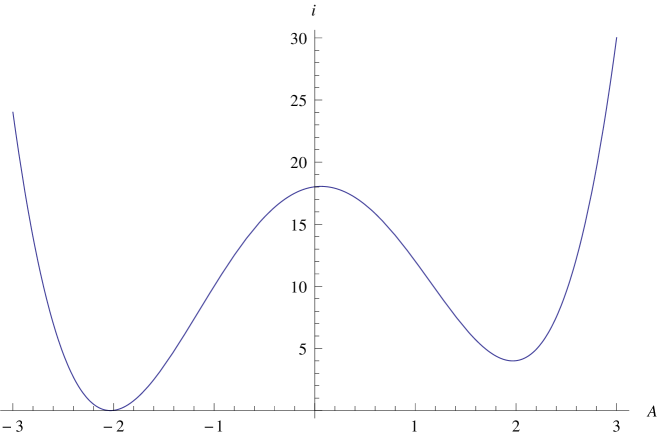
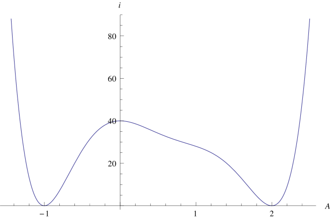
   Figure 2: $i(A)=(A^{2}-a^{2})^{2}+A+r$ with $a=2$ and $r=2.01539$

   

   Figure 3: $i(A)=7A^{6}-24A^{5}+9A^{4}+38A^{3}-42A^{2}+40$

2. Initial field: loss without recovery, with a “compensating” bad configuration. As an example we can take $i(A)=(A^{2}-a^{2})^{2}+A+r$. For $a>1$, this rate function has one local minimum in the vicinity of $x=a$, a maximum in the vicinity of $x=0$ and its (absolute) minimum in the vicinity of $x=-a$. This corresponds to an initial field (favorizing the minimizer $x=-a$). $i(A)$ with $a=2$ with $r=2.01539$ is plotted in Figure 3. The minimization of ${\mathscr{E}}_{b,T}(A)$ leads to the equation

   $$4A^{3}+2\alpha(a,T)A=\frac{b}{T}-1$$ (16)

   By an analysis of (16) similar for (14), we obtain that there is no bad point when $T\leq T_{crit}=\frac{1}{4a^{2}}$, but $b=T$ is bad for all $T>T_{crit}$. The bad point “compensates” the initial field, and therefore has to become larger (and positive) when time $T$ increases.

3. Non-symmetric rate function. To see that the symmetry of the initial rate function is not a necessary requirement to produce bad configurations, we have the following example. Let $i(A)=7A^{6}-24A^{5}+9A^{4}+38A^{3}-42A^{2}+40$ (see Figure 3). This rate function has two global minima at $x=-1$ and $x=2$ and one maximum at $x=0$. The cost function corresponding to trajectories arriving at $b$ at time $T$ is

   $${\mathscr{E}}_{b,T}(A)=7A^{6}-24A^{5}+9A^{4}+38A^{3}+\left(\frac{1}{2T}-42\right)A^{2}-\frac{b}{T}A+\frac{b^{2}}{2T}+40$$

   For fixed $b$, and $T$ large enough, this function has two local minima, located at $A^{1}(b,T)<A^{2}(b,T)$. Let us denote, for fixed $T$,

   $$D_{T}(b)={\mathscr{E}}_{b,T}(A^{1}(b,T))-{\mathscr{E}}_{b,T}(A^{2}(b,T))$$

   If as a function of $b$, $D_{T}$ changes sign, by continuity, there must be a value of $b^{*}$ where $D_{T}(b^{*})=0$, i.e., where the minima of ${\mathscr{E}}_{b^{*},T}$ are at equal height. This $b^{*}$ is then a bad point at time $T$. For $T=1$ we have $D_{T}(0.499)\approx-0.00182497<0$ and $D_{T}(0.4999)\approx 0.000868034>0$, so at $T=1$, there is a bad point at $b^{*}\in(0.499,0.4999)$. We observe that $b^{*}$ is $T$ dependent and tends to $0.5$ as $T$ increases. From numerical oberservations, we have $b^{*}\in(0.4999,0.49999)$ for $T=4$, $b^{*}\in(0.49999,0.499999)$ for $T=39$ and $b^{*}\in(0.499999,0.4999999)$ for $T=1000$.

4. General symmetric rate function. For any rate function $i(A)$ which is symmetric with respect to $x=0$ and which has minima for $A\neq 0$, $b=0$ is bad when $T$ is large enough. Indeed, the cost to arrive at $0$ is from (15): $i(A)+\frac{A^{2}}{2T}$ which has a non zero minimum as soon as $T$ is large enough.

5. General short-time Gibbsianness. For every rate function $i$ which is twice differentiable and its second derivative is continuous and bounded from below, we show that for $T$ small enough there is a unique minimum $A_{b}$ of ${\mathscr{E}}_{b,T}(A)$. This is the analogue of “short-time” Gibbsianness obtained in the lattice case via cluster expansions [11] or conditional Dobrushin uniqueness [12] and can be proved as follows.

   We look at the equation (see (15))

   $$i^{\prime}(A)=-\frac{A}{T}+\frac{b}{T}=:f(A).$$ (17)

   Put $d=\inf_{A}i^{\prime\prime}(A)$. Then we conclude, for

   $$T<-\frac{1}{d},$$ (18)

   that (17) has only one real solution $A_{b}$. Indeed, look at any two adjacent intersection points $A_{1}$ and $A_{2}$ of $i^{\prime}(A)$ and $f(A)$ if there were more than one real solution for (17). By the intermediate value theorem, we get

   $$\min(i^{\prime\prime}(A_{1}),i^{\prime\prime}(A_{2}))<-\frac{1}{T}<d=\inf_{A}i^{\prime\prime}(A).$$ (19)

   This is a contradiction. And further because $i^{\prime\prime}(A_{b})>-\frac{1}{T}$, we have

   $${\mathscr{E}}_{b,T}^{\prime\prime}(A_{b})=i^{\prime\prime}(A_{b})+\frac{1}{T}>0.$$ (20)

   Therefore $A_{b}$ is a minimum.

6. Non-Gibbsianness for all times. An example where $b=0$ is bad for all $T>0$ is $i(0)=0$, $i(A)=\int_{0}^{|A|}|x|\cos^{2}\frac{1}{x}dx$ for $A\neq 0$. This follows from the facts that $i^{\prime\prime}(A)$ is not bounded from below when $A\rightarrow 0$ and $i(A)$ is symmetric about $A=0$. To see that indeed for all $T>0$ $0$ is a bad point, we see that the line $f(A)=-A/T$ always intersects the graph of the derivative of the rate function.

4 Ornstein-Uhlenbeck process

As a second example, we consider the process $X^{n}_{t}$ to be the solution of

$$dX_{t}=-\kappa X_{t}+\frac{1}{\sqrt{n}}dB_{t}$$

and the initial point distributed as in the previous section, in (7), (8).

The cost function for the large deviation principle of the trajectories now becomes

$${\mathscr{I}}(\gamma)=i(\gamma_{0})+\frac{1}{2}\int_{0}^{T}(\dot{\gamma}_{s}+\kappa\gamma_{s})^{2}ds$$ (21)

The Euler-Lagrange trajectories extremizing $\frac{1}{2}\int_{0}^{T}(\dot{\gamma}_{s}+\kappa\gamma_{s})^{2}ds$ are given by

$$\gamma_{t}=Ae^{\kappa t}+Be^{-\kappa t}$$

by the terminal condition $\gamma_{T}=0$ we have

$$\gamma_{t}=-Be^{-2\kappa T}e^{\kappa t}+Be^{-\kappa t}$$

the cost function for such a trajectory can then explicitly be evaluated and gives

$${\mathscr{E}}_{0,T}(B)=c_{1}B^{4}+c_{2}B^{2}+c_{3}$$ (22)

where

$$c_{1} = (1-e^{-2\kappa t})^{4}$$

$$c_{2} = \left(-2a^{2}(1-e^{-2\kappa t})^{2}+\kappa e^{-2\kappa t}(1-e^{-2\kappa t})\right)$$

$$c_{3} = a^{4}$$ (23)

A similar analysis as in the previous section can now be started. We have a unique minimum at $B=0$ of the cost function ${\mathscr{E}}$ for

$$T\leq T_{crit}:=-\frac{1}{2\kappa}\log\left(\frac{2a^{2}}{2a^{2}+\kappa}\right)$$ (24)

and for $T>T_{crit}$, $0$ becomes the unique bad point for this process.

The cost of an optimal trajectory ending up at $b$ at time $T$ can also be expressed as a function of the starting point $\gamma_{0}$, which gives the explicit expression

$${\mathscr{E}}_{b,T}(\gamma_{0})=i(\gamma_{0})+\frac{\kappa}{e^{2\kappa T}-1}(\gamma_{0}-be^{\kappa T})^{2}$$ (25)

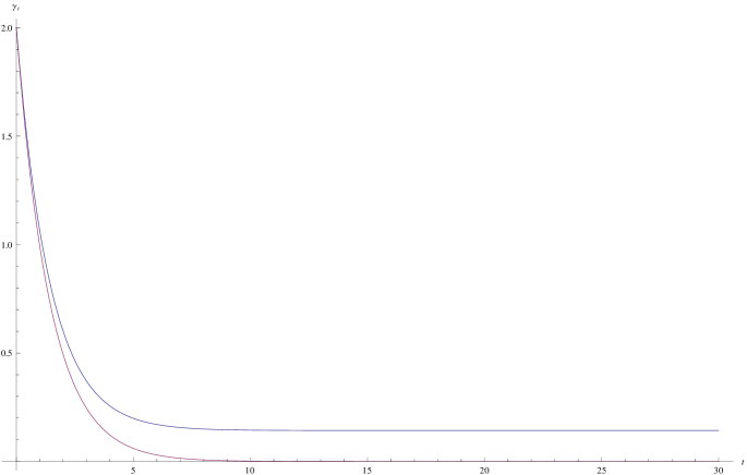
Figure 4: A limiting process (the purple line) with $a=2,\kappa=0.7,T=30$, hence $\gamma_{0}^{+}\approx 2.0$, and a corresponding conditioned process (the blue line) with $E=0.1$, $b\approx 0.142857$

4.1 Ornstein-Uhlenbeck process with constant external field

The equation for the process $X^{n}_{T}$ then reads

$$dX^{n}_{t}=(-\kappa X_{t}+E)dt+\frac{1}{\sqrt{n}}dB_{t}$$ (26)

where $E>0$ is a constant representing a (constant) external field. As rate function of the initial measure we choose as before (8). The cost of the trajectory is now given by $\int_{0}^{T}L(\gamma_{s},\dot{\gamma}_{s})ds$ with $L(\gamma_{s},\dot{\gamma}_{s})=(\dot{\gamma_{s}}+\kappa\gamma_{s}-E)^{2}$. The Euler-Lagrange trajectories are of the form

$$\gamma_{t}=Ae^{\kappa t}+Be^{-\kappa t}+\frac{E}{\kappa}$$

The trajectory cost of an Euler-Lagrange trajectory is given by $2A^{2}(e^{2\kappa T}-1)$. From this, we derive that the total cost of a trajectory to end up at time $T$ in $\gamma_{T}=b$ is given, as a function of $\gamma_{0}$, by

$${\mathscr{E}}^{E}_{b,T}(\gamma_{0})=i(\gamma_{0})+\frac{\kappa\left(\gamma_{0}-\left(b-\frac{E}{\kappa}\right)e^{\kappa T}-\frac{E}{\kappa}\right)^{2}}{e^{2\kappa T}-1}$$

The same analysis can then be performed. The “critical” time at which a unique bad point starts to appear is the same as in the zero field case, i.e., given by (24). This bad point is given by

$$b=\frac{E}{\kappa}(1-e^{-\kappa T})$$ (27)

which corresponds to the point at which the deterministic evolution $\dot{x}_{t}=-\kappa x_{t}+E$ arrives when starting from $x_{0}=0$. Notice that total cost to arrive at this bad point $b$ is given by

$$i(\gamma_{0})+\frac{\kappa\gamma_{0}^{2}}{e^{2\kappa T}-1}$$

which is symmetric around $\gamma_{0}=0$. Moreover, for $T$ large the path cost contribution which is equal to $\frac{\kappa\gamma_{0}^{2}}{e^{2\kappa T}-1}$ vanishes exponentially fast, and hence for large $T$ two minima exist.

The corresponding optimal trajectories to arrive at the bad point $b$ are starting from

$$\gamma_{0}^{\pm}=\pm\sqrt{a^{2}-\frac{\kappa}{2(e^{2\kappa T}-1)}}$$

and explicitly given by

$$\gamma_{t}=\left(b-\frac{E}{\kappa}\right)\frac{\sinh(\kappa t)}{\sinh(\kappa T)}+\left(\gamma_{0}-\frac{E}{\kappa}\right)\frac{\sinh(\kappa(T-t))}{\sinh(\kappa T)}+\frac{E}{\kappa}$$

The trajectory with plus resp. minus sign can be selected by conditioning to arrive at $b^{+}>b$, resp. $b^{-}<b$, and letting $b^{+}\to b$, resp. $b^{-}\to b$. Here we plot a limiting process with $a=2,\kappa=0.7,T=30$, hence $\gamma_{0}^{+}\approx 2.0$, and a corresponding conditioned process with $E=0.1$, hence $b\approx 0.142857$, see Figure 4.

4.2 General drift.

Let us now consider the process $X^{n}_{t}$ with a general drift $f(x)$ and variance $\frac{1}{n}$, i.e., the solution of

$$dX_{t}=-f(X_{t})dt+\frac{1}{\sqrt{n}}dB_{t}$$

We assume $f:\mathbb{R}\to\mathbb{R}$ to be Lipschitz, and odd: $f(-x)=-f(x)$. For the rate function of the initial point $X^{n}_{0}$ we choose as before (7), (8). The rate function of the trajectory is now given by

$${\mathscr{I}}(\gamma)=\frac{1}{2}\int_{0}^{T}(\dot{\gamma}_{s}+f(\gamma_{s}))^{2}ds$$ (28)

and the minimization problem for the optimal trajectory ending at zero $\gamma_{T}=0$ becomes now to find

$$\arg\min\{{\mathscr{I}}(\gamma)+i(\gamma_{0}):\gamma_{T}=0\}$$ (29)

The Euler-Lagrange equations for miminal cost trajectories are given by

$$\frac{d^{2}\gamma_{s}}{ds^{2}}=f(\gamma_{s})f^{\prime}(\gamma_{s})$$

These equations correspond to classical motion in a potential $U$ satisfying $U^{\prime}=-ff^{\prime}$, which gives as a possible choice $U=-\frac{1}{2}f^{2}$. Notice that this formal potential $U$ has no physical meaning, but we need it if we want to translate the framework of the Euler-Lagrange equations to Hamilton equations. Indeed, the corresponding Hamiltonian is

$$H(p,q)=\frac{p^{2}}{2}-U(q)$$ (30)

In particular, under the Euler-Lagrange equations,

$$\frac{\dot{\gamma}^{2}_{t}}{2}-\frac{1}{2}(f(\gamma_{t}))^{2}=E$$ (31)

is a constant of motion. Further, we have the open-end and terminal condition

$$i^{\prime}(\gamma_{0}) = \dot{\gamma_{0}}+f(\gamma_{0})$$

$$\gamma_{T} = 0$$ (32)

We can think of these equations as having $\gamma_{0}$ and $E$ as parameters. The terminal condition gives then a relation between $E$ and $\gamma_{0}$. Notice that the trajectory of zero-energy, $E=0$, $\gamma\equiv 0$ is always a solution since $f(0)=0$. We want to show that under some reasonable assumptions, for $T$ small, it is the only solution. For this we make the following assumptions. Call ${\mathscr{S}}_{T}(E)$ the collection of all trajectories $\gamma:[0,T]\to\mathbb{R}$ ending at $0$, i.e., with $\gamma_{T}=0$ and with “energy” $E$, i.e., such that

$$\frac{\dot{\gamma}^{2}_{t}}{2}-\frac{1}{2}(f(\gamma_{t}))^{2}=E$$

for all $0\leq t\leq T$. We impose now the following conditions.

1. There exist a function $\varphi:\mathbb{R}\to[0,\infty)$ and $T_{0}>0$ and a constant $C>0$ such that $\varphi(0)=0$, $\varphi(E)>0$ for $E\not=0$ such that for all $T\leq T_{0}$ and for all $\gamma\in{\mathscr{S}}_{T}(E)$, $\gamma_{0}\dot{\gamma}_{0}<0$,

   $$|\dot{\gamma}_{0}|\geq\varphi(E)$$ (33)

   and

   $$|\gamma_{0}|\leq C\varphi(E)T$$ (34)

2. The drift function $f$ is locally monotone around $0$, i.e., there exist $x_{0}$ such that $f$ restricted to $[0,x_{0}]$, $[-x_{0},0]$ is monotone.

The first condition states that if $T$ is small, and one wants to end at $\gamma_{T}=0$ from $\gamma_{0}>0$, then the derivative at zero should be negative, or vice versa. The second part of the condition states that there exist lower bounds for the derivative and upper bounds for $\gamma_{0}$.

Coming back to the previous examples: for the Brownian motion case, for all $\gamma\in{\mathscr{S}}_{T}(E)$ we have $\gamma_{t}=\pm\sqrt{2E}(t-T)$ hence and for $\gamma\in{\mathscr{S}}_{T}(E)$ we have $\gamma_{0}=\mp\sqrt{2E}T$, $\dot{\gamma}_{0}=\pm\sqrt{2E}$, and we can choose $\varphi(E)=\sqrt{2E}$. For the Ornstein-Uhlenbeck case we have $\gamma_{t}=B(e^{-\kappa t}-e^{-\kappa(2T-t)})$, $E=-2AB\alpha$ and if $\gamma_{T}=0$ we find $\gamma_{0}=\sqrt{2E/\kappa}\sinh(\kappa T)$, $\dot{\gamma}_{0}=-\sqrt{2E/\kappa}\cosh(\kappa T)$ which clearly satisfies the conditions, with the $\varphi=\sqrt{2E/\kappa}$.

The open-end condition requires

$$\dot{\gamma}_{0}+f(\gamma_{0})=4\gamma_{0}(\gamma_{0}^{2}-a^{2})$$

Hence, for $\gamma\in{\mathscr{S}}_{T}(E)$ such that $\gamma_{0}>0$:

$$-\varphi(E) \geq \dot{\gamma}_{0}$$ (35)

$$\geq 4\gamma_{0}(\gamma_{0}^{2}-a^{2})-f(C\varphi(E)T)$$

$$\geq 4C\varphi(E)T(C^{2}\varphi(E)^{2}T^{2}-a^{2})-f(C\varphi(E)T)$$

which is clearly a contradiction for $T$ sufficiently small. Hence for $T$ sufficiently small, there do not exist $E\not=0$ with $\gamma\in S_{T}(E)$. As a consequence, under these assumptions, for small $T$ the zero trajectory is the only solution of the minimization problem (29).

For large times, if we assume that the drift is such that from any starting point one can travel to the origin at arbitrary small cost if one has sufficient time, i.e., for all $x_{0}>0$,

$$\lim_{T\to\infty}\inf\left\{\int_{0}^{T}(\dot{\gamma}_{s}+f(\gamma)_{s})^{2}ds:\gamma_{0}=x_{0},\gamma_{T}=0\right\}=0$$

then this implies that for $T$ large enough that there exists $x_{0}\not=0$ and a trajectory $\gamma$ starting from $x_{0}$ such that $i(x_{0})<i(0)/2$ and

$$\left\{\int_{0}^{T}(\dot{\gamma}_{s}+f(\gamma)_{s})^{2}ds:\gamma_{0}=x_{0},\gamma_{T}=0\right\}<i(0)/2$$

this trajectory $\gamma$ clearly has lower cost than the zero trajectory, and by symmetry, $-\gamma$ is a trajectory with identical cost. Therefore, $0$ becomes a bad point.

5 Approximately deterministic walks in $d=1$

An “approximately deterministic random walk” is a continuous-time random walk with small increments performed at high rate, i.e., a random walk $X^{N}_{t}$ on $\mathbb{R}$ that, starting at $X_{0}=x$ makes increments of size $\pm 1/N$ with rates $Nb(x)$, resp. $Nd(x)$. In other words, $X^{N}_{t}$ is a Markov process on $\mathbb{R}$ with generator

$${\mathscr{L}}_{N}f(x)=Nb(x)\left(f\left(x+\frac{1}{N}\right)-f(x)\right)+Nd(x)\left(f\left(x-\frac{1}{N}\right)-f(x)\right)$$ (36)

Such walks arise naturally in the context of population dynamics see e.g. [7]. The notation $b(x)$ and $d(x)$ is also reminiscent of this interpretation and we will call these quantities birth resp. death rates.

We ask then the same large deviation question, i.e., we start the process $X^{N}_{t}$ from an initial distribution $\mu_{N}$ satisfying the large deviation principle with rate function (8) -or some natural modification of it if we have to restrict the state space- and look for the minimizing trajectory(ies) that end at time $T$ at the origin (or at a more general bad point if the dynamics has a drift see later).

The large deviation function for the trajectories can be computed using the Feng-Kurtz scheme, i.e., denoting $f^{N}_{p}(x)=e^{Npx}$ we computes the Hamiltonian

$${\mathscr{H}}(x,p)=\lim_{N\to\infty}\frac{1}{N}\left(\frac{1}{f^{N}_{p}}({\mathscr{L}}_{N}f^{N}_{p})\right)(x)=(e^{p}-1)b(x)+(e^{-p}-1)d(x)$$ (37)

and the corresponding Lagrangian

$$L(x,v)=\sup_{p\in\mathbb{R}}\left(pv-{\mathscr{H}}(x,p)\right)$$ (38)

For the trajectories of $\{X^{N}_{t}:0\leq t\leq T\}$, we have

$$\mathbb{P}(X^{N}_{.}\approx\gamma)\approx e^{-N\int_{0}^{T}L(\gamma_{s},\dot{\gamma}_{s})}ds$$ (39)

where the informal notation has to be interpreted as usual in the sense of the large deviation principle.

The equations for the optimal trajectories, i.e. for the minimizers of the “action”

$${\mathscr{I}}(\gamma)=i(\gamma_{0})+\int_{0}^{T}L(\gamma_{s},\dot{\gamma}_{s})ds$$ (40)

can now more conveniently be written in terms of the Hamiltonian (the Lagrangian is a more complicated expression to deal with).

Introducing the canonical coordinates $(x,p)$ we have the Hamilton equations, together with the terminal condition and the open-end condition corresponding to the choice of the distribution of $X^{N}_{0}$.

$$\dot{x}_{t} = \frac{\partial H}{\partial p}(x_{t},p_{t})=b(x)e^{p}-d(x)e^{-p}$$

$$\dot{p}_{t} = -\frac{\partial H}{\partial x}(x_{t},p_{t})=-b^{\prime}(x)(e^{p}-1)-d^{\prime}(x)(e^{-p}-1)$$ (41)

with conditions

$$x_{T} = 0$$

$$p_{0} = i^{\prime}(x_{0})=4x_{0}(x_{0}^{2}-a^{2})$$ (42)

The total “energy” is a constant of motion along minimizing trajectories, so we put $H(x,p)=E$ and we can rewrite the Hamilton equations (5)

$$E+b(x)+d(x)+\dot{x} = 2b(x)u$$

$$E+b(x)+d(x)-\dot{x} = 2d(x)u^{-1}$$ (43)

where $u=e^{p}$. Which leads to

$$\dot{x}^{2}=E^{2}+2E(b(x)+d(x))+(b(x)-d(x))^{2}$$ (44)

So we can think now of the cost of a trajectory as a function of two parameters: the starting point and the energy $(x_{0},E)$. Zero-energy correspond to the “typical trajectory” following the limiting differential equation $\dot{x}=b(x)-d(x)$, which means that the cost of the Lagrangian part of the rate function is zero, and only the cost due to the starting point $x_{0}$ has to be paid. Non-zero energy trajectories have a strictly positive cost of the Lagrangian part of the rate function. The additional terminal condition $X_{T}=b$ will eliminate one of these variables (e.g. $E$), so that we can think of the cost of the trajectory as a function of the single variable (e.g.) $x_{0}$.

We now concentrate on three important particular cases.

5.1 Constant birth and death rates

If $b$ and $d$ do not depend on $x$, then the equation for the momentum shows that $p_{t}=C$, hence we have linear Euler-Lagrange trajectories, and correspondingly the same analysis and phenomena as in the Brownian motion case of the previous section.

5.2 Mean-field independent spin flip

A special case, corresponding to independent spin flip dynamics is $b(x)=(1-x)$, $d(x)=(1+x)$. Moreover, the $x$-variable is now restricted to $[-1,1]$. As in the case $x\in\mathbb{R}$ we assume that initially, $x_{0}$ is distributed according to a measure $\mu_{n}(dx)$ on $[-1,1]$ satisfying the large deviation principle with the non-convex rate function (8) for $x\in[-1,1]$ and $+\infty$ otherwise. In particular, $a\in(0,1)$.

The Hamilton equations then read

$$\dot{x} = -x(e^{p}+e^{-p})+e^{p}-e^{-p}$$

$$\dot{p} = e^{p}-e^{-p}$$ (45)

Taking the derivative w.r.t. time of the first equation and using the second equation leads to elimination of $p$, and the simple second order equation for $x$: to

$$\frac{d^{2}x}{dt^{2}}=4x$$ (46)

with solutions

$$x(t)=C_{1}e^{2t}+C_{2}e^{-2t}$$

where $C_{1},C_{2}$ are determined by the open-end condition and the terminal condition. This case was treated before in the context of the Curie-Weiss model subjected to independent spin flips in [9], [11].

The equation for the momentum can be integrated and gives

$$\tanh(p_{t}/2)=\pm Ce^{2t}$$

Furthermore, since

$$E=(1-x)(e^{p}-1)+(1+x)(e^{-p}-1)$$

is a constant of motion, we find as possible solutions for $x$, using that $x_{T}=0$:

$$x_{t}=\pm\sqrt{E/4(1+E/4)}\left(e^{2(t-T)}-e^{2(T-t)}\right)$$

In particular, as in the Brownian motion case, the zero-energy trajectory ($E=0$) yields $x_{t}=0$. The relation between the energy, initial position and initial momentum is

$$p_{0}=\log\left(\frac{2+E+\sqrt{(2+E)^{2}-4(1-x_{0}^{2})}}{2(1-x_{0})}\right)$$

Zero-energy thus corresponds to zero initial momentum and zero initial position.

In general, the initial points are symmetrically distributed around the origin and related to the energy via

$$x_{0}=\pm\sqrt{E/4(1+E/4)}\left(e^{-2T}-e^{2T}\right)$$

Whether or not a non-zero energy solution can be the minimizer is determined by the open-end condition:

$$p_{0}=i^{\prime}(x_{0})=4x_{0}(x_{0}^{2}-a^{2})$$ (47)

This can be viewed now as an equation for $E$. For small $T>0$,

$$x_{0}=x_{0}(E,T)\approx C(E)T,p_{0}=p_{0}(E,T)\approx cE$$

which implies that a non-zero energy solution of (47) can not exist for small $T$. For large $T$, a non-zero energy solution exists yielding two symmetrically solution for $x_{0}$.

Alternatively, the trajectory cost $C_{T}(\gamma_{0})$ of a trajectory starting at $\gamma_{0}$ ending up at time $T$ at $b=0$ has the following important properties

1. Symmetry: $C_{T}(-\gamma_{0})=C_{T}(\gamma_{0})$

2. Small time behavior: $\lim_{T\to 0}C_{T}(\gamma_{0})=\infty$ for all $\gamma_{0}\not=0$

3. Large time behavior: $\lim_{T\to\infty}C_{T}(\gamma_{0})=0$ for all $\gamma_{0}$

From these properties it follows that for small $T$ there are no bad points, and for large $T$ zero is the unique bad point. Notice that contrary to the Curie Weiss model situation analyzed in [9] there are no non-neutral (non-zero) bad configurations due to the fact that the rate function of the initial measure is here simply a fourth order polynomial.

5.3 Independent spin-flips in a field

This corresponds to the choice $b(x)=\gamma(1-x)$, $d(x)=(1+x)$, $x\in[-1,1]$. Here $\gamma>1$ corresponds to a bias in the plus direction (positive magnetic field). The limiting deterministic trajectory is given by

$$\frac{dx_{t}}{dt}=-(1+\gamma)x_{t}+(\gamma-1)$$

$$x_{t}=x_{0}e^{-(1+\gamma)t}+\frac{\gamma-1}{1+\gamma}\left(1-e^{-(1+\gamma)t}\right)$$ (48)

This is the zero-energy trajectory starting from $x_{0}$.

Using (44) we find that for a given energy $E$, the solution for $x$ is of the form

$$x_{t}=x(E,C,t)=C_{1}e^{t(1+\gamma)}+C_{2}e^{-t(1+\gamma)}+C_{3}$$ (49)

with

$$C_{1} = \frac{C(2+2\gamma+E)}{(\gamma+1)^{2}}$$

$$C_{2} = \frac{E\gamma}{-C(1+\gamma)^{2})}$$

$$C_{3} = \left(\frac{(E+1+\gamma)(\gamma-1)}{(1+\gamma)^{2}}\right)$$ (50)

where $C$ is an integration constant.

REMARK 5.1.

1. Remark that for $E=0$ $C_{3}=(\gamma-1)(1+\gamma)^{-1}$ which corresponds to the limiting value of the zero energy trajectory.

2. If $\gamma=1$, and $E\not=0$ we find $C_{3}=0$ and recover the solution of the form $C_{1}e^{2t}+C_{2}e^{-2t}$ corresponding to the optimal trajectories of the independent spin flip dynamics.

The general form of an optimal trajectory arriving at time $T$ at $x_{T}=b$ and starting from $x_{0}=\gamma_{0}$ is

$$x(t)=(b-C_{3})\frac{\sinh(\delta t)}{\sinh(\delta T)}+(\gamma_{0}-C_{3})\frac{\sinh(\delta(T-t))}{\sinh(\delta T)}+C_{3}$$

with $\delta=(1+\gamma)$ and where $C_{3}$ is given in (5.3). Notice the analogy with the case of the Ornstein-Uhlenbeck process in a constant field (27). As in that case, the bad point is time-dependent and given by

$$b=\frac{\gamma-1}{\gamma+1}\left(1-e^{-\delta T}\right)$$

which is the point at which the limiting deterministic dynamics arrives at time $T$ when started from $x_{0}=0$. The trajectory cost $C_{T}(\gamma_{0})$ to arrive at this bad point satisfies the same properties as the trajectory cost $C_{T}(\gamma_{0})$ of the previous subsection (zero field case). Hence, for $T$ large two minimizing $\gamma_{0}$ of the total cost function appear which correspond to two optimal trajectories.

6 Acknowledgement

We thank Aernout van Enter and Olaf de Leeuw for useful discussions and suggestions.

References

- [1] A. Dembo and O. Zeitouni. Large deviations techniques and applications. Second edition, Springer Verlag, (2010).
- [2] D. Dereudre and S. Roelly, Propagation of Gibbsianness for infinite-dimensional gradient Brownian diffusions. J. Stat. Phys. 121, 511-551 (2005).
- [3] A.C.D. van Enter, R. Fernández, F. den Hollander and F. Redig, Possible loss and recovery of Gibbsianness during the stochastic evolution of Gibbs measures, Comm. Math. Phys. 226, 101-130 (2002).
- [4] A.C.D. van Enter, R. Fernández, F. den Hollander and F. Redig, A large-deviation view on dynamical Gibbs-non-Gibbs transitions, Mosc. Math. J. 10, 687-711 (2010).
- [5] A.C.D. van Enter, C. Külske, Alex A. Opoku and W.M. Ruszel, Gibbs-non-Gibbs properties for -vector lattice and mean field models, Braz. J. Probab. Stat. 24, 226-255 (2010).
- [6] A.C.D. van Enter and W.M. Ruszel, Gibbsianness versus non-Gibbsianness of time-evolved planar rotor models. Stochastic Process. Appl. 119, 1866-1888, (2009).
- [7] A. Etheridge, Evolution in fluctuating populations. Les Houches School on Mathematical Statistical Physics, pp. 489-545, Elsevier B. V., Amsterdam, (2006).
- [8] J. Feng and T.G. Kurtz, Large Deviations for Stochastic Processes, American Mathematical Society, Providence RI, (2006).
- [9] C. Külske and V. Ermolaev, Low-temperature dynamics of the Curie-Weiss model: periodic orbits, multiple histories, and loss of Gibbsianness. J. Stat. Phys. 141, 727-756, (2010).
- [10] C. Külske and F. Redig, Loss without recovery of Gibbsianness during diffusion of continuous spins. Prob. Theory Rel. Fields 135, 428-456 (2006).
- [11] A. Le Ny and F. Redig, Short-time conservation of Gibbsianness under local stochastic evolutions. J. Statist. Phys. 109, 1073-1090 (2002).
- [12] C. Külske and Alex A. Opoku, The posterior metric and the goodness of Gibbsianness for transforms of Gibbs measures. Electron. J. Probab. 13, 1307-1344, (2008).