Nonmesonic Weak Decay of $\Lambda$-Hypernuclei within Independent-Particle Shell-Model

Abstract

After a short introduction to the nonmesonic weak decay (NMWD) $\Lambda N\rightarrow nN$ of $\Lambda$-hypernuclei we discuss the long-standing puzzle on the ratio $\Gamma_{n}/\Gamma_{p}$, and some recent experimental evidences that signalized towards its final solution. Two versions of the Independent-Particle-Shell-Model (IPSM) are employed to account for the nuclear structure of the final residual nuclei. They are: (a) IPSM-a, where no correlation, except for the Pauli principle, is taken into account, and (b) IPSM-b, where the highly excited hole states are considered to be quasi-stationary and are described by Breit-Wigner distributions, whose widths are estimated from the experimental data. We evaluate the coincidence spectra in ${}^{4}_{\Lambda}$He, ${}^{5}_{\Lambda}$He, ${}^{12}_{\Lambda}$C, ${}^{16}_{\Lambda}$O, and ${}^{28}_{\Lambda}$Si, as a function of the sum of kinetic energies $E_{nN}=E_{n}+E_{N}$ for $N=n,p$. The recent Brookhaven National Laboratory experiment E788 on ${}^{4}_{\Lambda}$He, is interpreted within the IPSM . We found that the shapes of all the spectra are basically tailored by the kinematics of the corresponding phase space, depending very weakly on the dynamics, which is gauged here by the one-meson-exchange-potential. In spite of the straightforwardness of the approach a good agreement with data is achieved. This might be an indication that the final-state-interactions and the two-nucleon induced processes are not very important in the decay of this hypernucleus. We have also found that the $\pi+K$ exchange potential with soft vertex-form-factor cutoffs $(\Lambda_{\pi}\approx 0.7$ GeV, $\Lambda_{K}\approx 0.9$ GeV), is able to account simultaneously for the available experimental data related to $\Gamma_{p}$ and $\Gamma_{n}$ for ${}^{4}_{\Lambda}$H, ${}^{4}_{\Lambda}$He, and ${}^{5}_{\Lambda}$He.

1 Introduction

The nonmesonic weak decay (NMWD) of $\Lambda$ hypernuclei, $\Lambda N\rightarrow nN$ ($N=p,n$), takes place only within nuclear environment. Without producing any additional on-shell particle (as does the mesonic weak decay $\Lambda\rightarrow\pi N$) the mass is changed by $176$ MeV, and the strangeness by $\Delta{\sf S}=1$, which implies that we are witnessing the most drastic metamorphosis of an elementary particle within the nucleus. As such, the hypernuclei can be considered as a powerful ”laboratory” for unique investigations of baryon-baryon strangeness- changing weak interactions, and the NMWD could play an important role in the stability of rotating neutron stars with respect to gravitational wave emission Da04 ; Ju08 .

Same as the free $\Lambda$ hyperon, they are mostly produced via the strong interactions, i.e., in the reaction processes $\pi^{+}n\rightarrow\Lambda K^{+}$, $K^{-}n\rightarrow\pi^{-}\Lambda$ and $K^{-}p\rightarrow\pi^{0}\Lambda$, by making use of the pion ($\pi$) and kaon ($K$) beams. They also basically decay through the weak interactions, as the free $\Lambda$ does. Yet, as it is well known and explained below, there are some very important differences in the corresponding decaying modes.

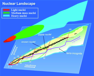
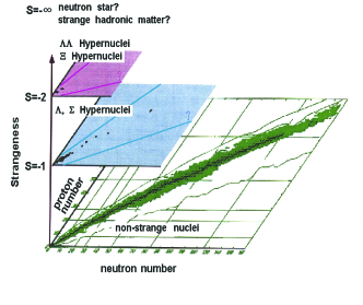
Figure 1: On the left and right panels are represented, respectively, the standard nuclear chart of nuclides, and the hypernuclear chart of isotopes. The NMWD corresponds to a jump from the surface $S=1$ in the three-dimensional chart $({\sf N,Z,S})$ to the standard $({\sf N,Z})$ chart.

Not less important is the fact that with the incorporation of strangeness, the radioactivity domain is extended to three dimensions $({\sf N,Z,S})$, as illustrated in Fig. 1. The best studied systems are nuclei containing a $\Lambda$-hyperon, which because of the additional binding are even richer in elements than the ordinary $({\sf N,Z})$ domain. (For instance, while the one-neutron separation energy in ²⁰C is $1.01$ MeV, it is $1.63$ MeV in ${}^{21}_{\Lambda}$C  Sa08 .) This attribute of hypernuclei has motivated a recent proposal to produce neutron rich $\Lambda$-hypernuclei at J-PARC, including ${}^{9}_{\Lambda}$He Sa09 . The shrinkage of the ²⁰C nucleus by the addition of an $\Lambda$-hyperon to build up the ${}^{21}_{\Lambda}$C hypernucleus is illustrated in Fig. 2.

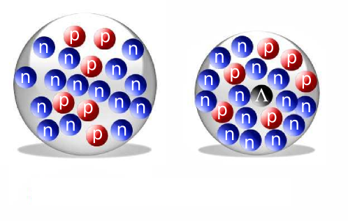
Figure 2: Pictorial representation of shrinkage of ²⁰C nucleus by the addition of an $\Lambda$-hyperon to build up the ${}^{21}_{\Lambda}$C hypernucleus.

The free $\Lambda$ hyperon decays (as represented schematically by the first graph in Fig. 3) nearly $100$ % of the time by the $\Lambda\rightarrow N\pi$ weak-mesonic mode

$$\Lambda\rightarrow\left\{\begin{array}[]{ccc}p+\pi^{-}&&(64.1\%)\\ n+\pi^{0}&&(35.7\%),\end{array}\right.$$

with the total transition rate $\Gamma^{0}_{\pi^{-}}+\Gamma^{0}_{\pi^{0}}=\Gamma^{0}=2.50\cdot 10^{-6}$ eV (which corresponds to the lifetime $\tau^{0}=2.63\cdot 10^{-10}$ sec). For the decay at rest the energy-momentum conservation implies

$$M_{\Lambda}=M_{N}+\frac{p_{N}^{2}}{2M_{N}}+\sqrt{p_{\pi}^{2}+m_{\pi}^{2}};~{}~{}~{}~{}p_{N} \equiv p_{\pi}.$$

Therefore the energy released is

$$Q_{0}=M_{\Lambda}-M_{N}-m_{\pi}\cong 37~{}\mbox{MeV},$$

and the kinetic energies and momenta in the final state are:

$$T_{N} = \frac{(M_{\Lambda}-M_{N})^{2}+m_{\pi}^{2}}{2M_{\Lambda}}\cong 5~{}\mbox{MeV};$$

$$T_{\pi} = Q_{0}-T_{N}\cong 32~{}\mbox{MeV},$$

$$p_{N} \equiv p_{\pi}=\sqrt{(T_{N}+M_{N})^{2}-M_{N}^{2}}\cong 100~{}\mbox{MeV}/c.$$

During the decay the isospin is changed by $\Delta T=1/2$ and $3/2$ and its projection by $\Delta M_{T}=-1/2$. However, as the above experimental data can be accounted for fairly well by neglecting the $\Delta T=3/2$ component, one end up with $\Delta T=1/2$ rule, which leads to the estimate $\Gamma_{\pi^{-}}/\Gamma_{\pi^{0}}=2$, while the experimental result is $64.1/35.7=1.80$.

Assuming the $\Delta T=1/2$ rule, the phenomelogical weak Hamiltonian for the process depicted in Fig. 31 can be expressed as:

$$H_{W} = -iG_{F}m_{\pi}^{2}\overline{\psi}_{N}\left(A_{\pi}+B_{\pi}\gamma_{5}\right)\mbox{\boldmath$\phi$}_{\pi}\cdot\mbox{\boldmath$\tau$}\psi_{\Lambda}\left(\negthinspace\begin{array}[]{c}0\\ 1\end{array}\right),$$ (4)

where $G_{F}m_{\pi}^{2}=2.21\times 10^{-7}$ is the weak coupling constant. The empirical constants $A_{\pi}=1.05$ and $B_{\pi}=-7.15$, adjusted to the observables of the free $\Lambda$ decay, determine the strengths of parity violating and parity conserving amplitudes, respectively. The nucleon, $\Lambda$ and pion fields are given by $\psi_{N}$ and $\psi_{\Lambda}$ and $\mbox{\boldmath$\phi$}_{\pi}$, respectively, while the isospin spurion $\left(\negthinspace\begin{array}[]{c}0\\ 1\end{array}\right)$ is included in order to enforce the empirical $\Delta T={1/2}$ rule.

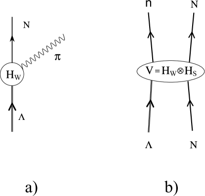
Figure 3: Schematic representation of: a) mesonic (nonleptonic) decay $\Lambda\rightarrow N+\pi$ induced by the weak vertex $H_{W}$, and b) nonmesonic weak decay $\Lambda N\rightarrow nN$, engendered by the product of a weak vertex $H_{W}$ and a strong vertex $H_{S}$.

The free $\Lambda$ hyperon weak decay is radically modified in the nuclear environment because the nucleon and the hyperon now move, respectively, in the mean fields $U_{N}$ and $U_{\Lambda}$, which come from the $NN$ and $N\Lambda$ interactions. $U_{N}$ and $U_{\Lambda}$ are characterized by the single particle energies (s.p.e.) $\varepsilon_{N}$ and $\varepsilon_{\Lambda}$, and we have to differentiate between:

$\bullet$ Mesonic Weak Decay (MWD): The basic process is again represented by the first graph shown in Fig. 3, and described by the hamiltonian (4). Yet, the energy-momentum conservation is different:

$$M_{\Lambda}=M_{N}-\varepsilon_{\Lambda}+\varepsilon_{N}^{\uparrow}+\frac{p_{\pi}^{2}}{2(A-1)M_{N}}+\sqrt{p_{\pi}^{2}+m_{\pi}^{2}},$$ (5)

where $A$ is the mass number, and $\varepsilon_{N}^{\uparrow}$ are the s.p.e. of the loosely bound states above the Fermi energy $\varepsilon_{N}^{F}$. They are of the order of a few MeV, while $\varepsilon_{\Lambda}$ is the energy of the $0s_{1/2}$ state and goes from $-11.7$ MeV for ${}^{13}_{\Lambda}$C to $-26.5$ MeV for ${}^{208}_{\Lambda}$ Pb Us99 . Thus, the corresponding Q-values

$$Q_{M}=M_{\Lambda}-M_{N}-m_{\pi}+\varepsilon_{\Lambda}-\varepsilon_{N}^{\uparrow},$$ (6)

are significantly smaller than $Q_{0}$, particularly for medium and heavy nuclei. This small value of $Q_{M}$ makes, as illustrated in (Kr03, , Fig. 2), the MWD to be hindered due to the Pauli principle. In fact, the experimental decay rates $\Gamma_{\pi^{-}}+\Gamma_{\pi^{0}}=\Gamma_{M}\equiv\Gamma_{M}(\Lambda\rightarrow N\pi$) are of the order of $\Gamma^{0}$ only for nuclei with $A\leq 4$, and they rapidly fall as a function of nuclear mass. For instance, in ${}^{12}_{\Lambda}$ C: $\Gamma_{\pi^{0}}/\Gamma^{0}=0.217\pm 0.084$ and $\Gamma_{\pi^{-}}/\Gamma^{0}=0.052^{+0.063}_{-0.035}$. (For a recent theoretical study of the MWD see Ref. Ga09 .)

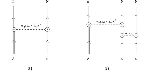
Figure 4: a) One-nucleon, and b) two-nucleon induced $\Lambda$-decay in nuclei. Strictly speaking the OME diagrams are only valid for nonstrange-mesons $\pi,\rho,\omega$, and $\eta$. For strange-mesons $K$, and $K^{*}$ the vertices $W$, and $S$ should be exchanged, i.e., $W\rightarrow S$, and $S\rightarrow W$.

$\bullet$ Nonmesonic Weak Decay (NMWD): New nonmesonic decay channels $\Lambda N\rightarrow nN$ become open inside the nucleus, where there are no pions in the final state; it is represented schematically by the second diagram in Fig. 3. The corresponding transition rates can be stimulated either by protons, $\Gamma_{p}\equiv\Gamma(\Lambda p\rightarrow np)$, or by neutrons, $\Gamma_{n}\equiv\Gamma(\Lambda n\rightarrow nn)$. The energy-momentum conservation and the Q-value are, respectively:

$$M_{\Lambda} = M_{N}-\varepsilon_{\Lambda}-\varepsilon_{N}^{\downarrow}+\frac{p_{n}^{2}}{2M_{N}}+\frac{p_{N}^{2}}{2M_{N}}+\frac{|{\bf p}_{n}+{\bf p}_{N}|^{2}}{2M_{N}(A-2)},$$ (7)

and

$$Q_{NM}=M_{\Lambda}-M_{N}+\varepsilon_{\Lambda}+\varepsilon_{N}^{\downarrow}.$$ (8)

Since the mean energy of the bound single-particle states is $\varepsilon_{N}^{\downarrow}\sim-30$ MeV, the Q-value is $Q_{NM}\sim 120-135$ MeV, and this is basically the kinetic energy of the two particles that are ejected from the hypernucleus. Therefore, the NMWD possesses a large phase space in the continuum, as illustrated in (Kr03, , Fig. 3), and the momenta ${\bf p}_{n}$, and ${\bf p}_{N}$ of two outgoing nucleons are relatively large ($\sim 420$ MeV). Therefore, the non-mesonic mode is not blocked by the Pauli principle, and dominates over the mesonic mode for all but the $s$-shell hypernuclei.

It is assumed very often that the hypernuclear NMWD $\Lambda N\rightarrow nN$ is triggered via the exchange of a virtual meson, and the obvious candidate is the one-pion-exchange (OPE) mechanism, where the strong Hamiltonian

$$H_{S}^{\pi} = ig_{NN\pi}\bar{\psi}_{N}\gamma_{5}\mbox{\boldmath$\pi$}\cdot\mbox{\boldmath$\tau$}\psi_{N},$$ (9)

with $g_{NN\pi}=13.4$, accompanies the weak Hamiltonian (4) Ad67 .

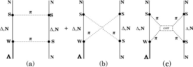
Figure 5: (a) direct, and (b) crossed uncorrelated, and (c) correlated two-pion-exchange diagrams for the weak $\Lambda N\rightarrow nN$ transition amplitude.

Later on, the full one meson-exchange (OME) model has been introduced by Dubach et al.  Du96 , as schematically represented by the first graph in Fig. 4. Also are considered frequently the two-nucleon induced NMWD, represented by the second diagram in in Fig. 4. Here, one or two bound nucleons are expelled to the continuum by the nuclear ground state correlations, and one of them, together with the hyperon $\Lambda$, exchanges one meson giving rise to three decaying nucleons, i.e., $\Lambda nN\rightarrow nNN$. The corresponding decay rate is denoted as $\Gamma_{2}$, and the total weak decay rate of a $\Lambda$-hypernucleus is then:

$$\Gamma_{T}=\Gamma_{M}+\Gamma_{NM},$$ (10)

where:

$$\Gamma_{M}=\Gamma_{\pi^{-}}+\Gamma_{\pi^{0}},~{}~{}\Gamma_{NM}=\Gamma_{1}+\Gamma_{2},~{}~{}\Gamma_{1}=\Gamma_{n}+\Gamma_{p}.$$ (11)

The OME potential is sometimes complemented with the contributions of uncorrelated ($2\pi$) and correlated ($2\pi/\sigma$) two-pion-exchange Ch07 , which are illustrated in see Fig. 5.

2 $\Gamma_{n}/\Gamma_{p}$ puzzle

Large experimental values of the ratio $\Gamma_{n/p}=\Gamma_{n}/\Gamma_{p}$ in ${}^{5}_{\Lambda}$He and ${}^{12}_{\Lambda}$C, measured before the year $2003$ Sz91 ; No95 ; Ha02 , were a cumbersome puzzle for the theorists during almost two decades, as schematically represented in Fig. 6. In fact, following the pioneering investigations of Adams Ad67 several calculations have been done within OPE coupling scheme of the total NMWD rate, and the ratio $\Gamma_{n/p}=\Gamma_{n}/\Gamma_{p}$ reproducing reasonably well the first one, but failing badly for the second observable. (see Refs. Os98 ; Al02 ; Al04 ; Pa07 ; Ch08 , and references therein).

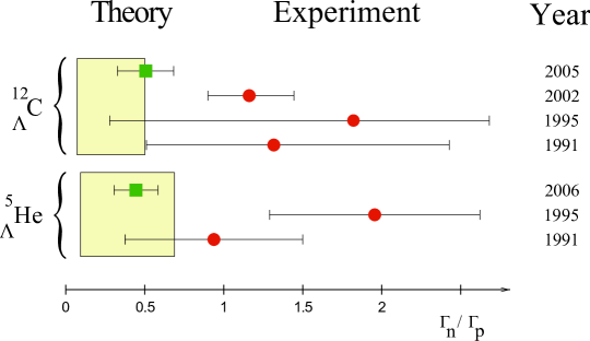
Figure 6: $\Gamma_{n}/\Gamma_{p}$ puzzle: The experimental values of the ratio $\Gamma_{n/p}$ are: a) ${}^{5}_{\Lambda}$He $\Gamma_{n/p}=0.93\pm 0.55$ (BNL) Sz91 , $1.97\pm 0.67$ (KEK) No95 , $0.45\pm 0.11\pm 0.03$ (KEK-E462) Ka06 , and b) ${}^{12}_{\Lambda}$C: $\Gamma_{n/p}=1.33^{+1.12}_{-0.81}$ (BNL) Sz91 , $1.87\pm 0.59^{+0.32}_{-1.00}$ (KEK) No95 , $1.17^{+0.09+0.20}_{-0.08-0.18}$ (KEK) Ha02 , $0.51\pm 0.13\pm 0.05$ (KEK) Ki03 ; Ki06 , while the theoretical estimates for $\Gamma_{n/p}$ vary between $0.09$ and $0.70$ for ${}^{5}_{\Lambda}$He, and between $0.08$ and $0.50$ for ${}^{12}_{\Lambda}$C.

The deficiency of the OPE model was attributed to effects of short range physics, which should be quite important in view of the large momentum transfers involved. Although there have been some attempts to account for this fact by making use of quark models to compute the shortest range part of the transition potential Che83 ; Ma94 ; In96 ; In98 ; Sa00 , most of the theoretical work opted for the addition of other, heavier mesons in the exchange process Mc84 ; Du96 ; Ta85 ; Na88 ; Pa95a ; Ra91 ; Ra92 ; Pa95 ; Pa97 ; Ha01 ; Pa01 ; Ba02 ; Sa02 ; Ba03 ; Bau03 ; Ba05 ; Kr03 . None of these models gives fully satisfactory results. Inclusion of correlated two-pion exchange has not been completely successful either Sh94 ; It02 . Nor have the addition of uncorrelated two-pion exchange, two-nucleon induced transitions or medium effects, treated within the nonrelativistic Os85 ; Al91 ; Ra94 ; Ra97a ; Al02 ; Ji01 or relativistic Zh99 propagator approaches, been of much help.

Yet, several important experimental advances in NMWD have been made in recent years, which have allowed to establish more precise values of the neutron- and proton-induced transition rates $\Gamma_{n}$ and $\Gamma_{p}$, solving in this way the long-standing puzzle of the branching ratio $\Gamma_{n/p}$. They are: 1) the new high quality measurements of single-nucleon spectra $S_{N}(E)$, as a function of one-nucleon energy $E_{N}\equiv E$ done in Refs. Ki03 ; Ok04 ; Par07 ; Ag08 , and 2) the first measurements of the two-particle-coincidence spectra as a function of the sum of kinetic energies $E_{n}+E_{N}\equiv E$, $S_{nN}(E)$, and of the opening angle $\theta_{nN}\equiv\theta$, $S_{nN}(\cos\theta)$, done in Refs. Ok05 ; Ou05 ; Ka06 ; Ki06 ; Bh07 ; Par07 .

3 Transition Rates

To derive the NMWD rate we start from the Fermi Golden Rule. For a hypernucleus (in its ground state with spin $J_{I}$ and energy $E_{J_{I}}$) to residual nuclei (in the several allowed states with spins $J_{F}$ and energies $E_{\alpha_{N}J_{F}}$) and two free nucleons $nN$ (with total spin $S$ and total kinetic energy $E_{nN}=E_{n}+E_{N}$), reads

$$\Gamma_{N} = 2\pi\sum_{S\alpha_{N}J_{F}}\int|\langle{\bf p}_{n}{\bf p}_{N}S;\alpha_{N}J_{F}|V|J_{I}\rangle|^{2}\delta(\Delta_{\alpha_{N}J_{F}}-E_{R}-E_{nN})\frac{d{\bf p}_{n}}{(2\pi)^{3}}\frac{d{\bf p}_{N}}{(2\pi)^{3}},$$ (12)

where for the sake of simplicity we have suppressed the magnetic quantum numbers. The NMWD dynamics, contained within the weak hypernuclear transition potential $V$, will be described by the OME model, whose most commonly used version includes the exchange of the full pseudoscalar ($\pi,K,\eta$) and vector ($\rho,\omega,K^{*}$) meson octets (PSVE), with the weak coupling constants obtained from soft meson theorems and $SU(6)_{W}$ Pa97 ; Du96 . The wave functions for the kets $|{\bf p}_{n}{\bf p}_{N}SM_{S}J_{F}M_{F}\rangle$ and $|J_{I}M_{I}\rangle$ are assumed to be antisymmetrized and normalized, and the two emitted nucleons $n$ and $N$ are described by plane waves. Initial and final short range correlations are included phenomenologically at a simple Jastrow-like level, while the finite nucleon size effects at the interaction vertices are gauged by monopole form factors Pa97 ; Ba02 . Moreover,

$$E_{R}=\frac{|\bm{p}_{n}+\bm{p}_{N}|^{2}}{2M(A-2)}=\frac{E_{nN}+2\cos\theta_{nN}\sqrt{E_{n}E_{N}}}{A-2},$$ (13)

is the recoil energy of the residual nucleus, and

$$\Delta_{\alpha_{N}J_{F}}=\Delta M+E_{J_{I}}-E_{\alpha_{N}J_{F}},\hskip 28.45274pt\mbox{with}\hskip 28.45274pt\Delta M=M_{\Lambda}-M=176~{}~{}\mbox{MeV},$$ (14)

is the liberated energy.

It could be convenient to perform a transformation to the relative and c.m. momenta (${\bf p}=\frac{1}{2}({\bf p}_{n}-{\bf p}_{N}$), ${\bf P}={\bf p}_{n}+{\bf p}_{N}$), coordinates (${\bf r}={\bf r}_{n}-{\bf r}_{N}$, ${\bf R}=\frac{1}{2}({\bf r}_{n}+{\bf r}_{N})$) and orbital angular momenta $\bm{l}$ and $\bm{L}$, and to express the energy conservation as

$$E_{nN}+E_{r}-\Delta_{\alpha_{N}J_{F}}={\epsilon}_{p}+{\epsilon}_{P}-\Delta_{\alpha_{N}J_{F}}=0,$$ (15)

where

$${\epsilon}_{p}=\frac{p^{2}}{M},\hskip 28.45274ptE_{r}=\frac{P^{2}}{2M(A-2)},\hskip 28.45274pt{\epsilon}_{P}=\frac{P^{2}}{4M}\frac{A}{A-2}=\frac{A}{2}E_{r},$$ (16)

are, respectively, the energies of the relative motion of the outgoing pair, of the recoil, and of the total c.m. motion (including the recoil).

Following the analytical developments done in Ref. Ba02 , the transition rate can be expressed as a function of the c.m. energy ${\epsilon}_{P}$:

$$\Gamma_{N} = \frac{16M^{3}}{\pi}\left(\frac{A-2}{A}\right)^{3/2}\int_{0}^{\Delta}d{\epsilon}_{P}\sum_{\alpha_{N}J_{F}}\sqrt{{\epsilon}_{P}(\Delta_{\alpha_{N}J_{F}}-{\epsilon}_{P})}\mathcal{F}_{\alpha_{N}J_{F}}(pP).$$ (17)

It is understood that the square root should be replaced by zero whenever its argument is negative. Here

$$\mathcal{F}_{\alpha_{N}J_{F}}(pP) = \hat{J}_{I}^{-2}\sum_{S\lambda lLTJ}\left|\sum_{j_{N}}{{\cal M}}(plPL\lambda SJ\mathsf{T};j_{\Lambda}j_{N}J\mathsf{t}_{\Lambda N})\langle J_{I}||\left(a_{j_{N}}^{\dagger}a_{j_{\Lambda}}^{\dagger}\right)_{J}||\alpha_{N}J_{F}\rangle\right|^{2},$$

and

$${{\cal M}}(plPL\lambda SJ\mathsf{T};j_{\Lambda}j_{N}J\mathsf{t}_{\Lambda N}) = \frac{1}{\sqrt{2}}\left[1-(-)^{l+S+T}\right]$$ (19)

$$\times ({plPL\lambda SJ\mathsf{T}}|V|{j_{\Lambda}j_{N}J\mathsf{t}_{\Lambda N}}).$$

$\mathsf{T}\equiv\{TM_{T},M_{T}=m_{t_{\Lambda}}+m_{t_{N}}\}$, $\mathsf{t}_{\Lambda N}\equiv\{t_{\Lambda}=1/2,m_{t_{\Lambda}}=-1/2,t_{N}=1/2,m_{t_{N}}\}$, with $m_{t_{p}}=1/2$, and $m_{t_{n}}=-1/2$, and $l$ and $L$ stand for quantum numbers of the relative and c.m. orbital angular momenta in the $\Lambda N$ system. The transition matrix elements ${{\cal M}}(plPL\lambda SJ\mathsf{T};j_{\Lambda}j_{N}J\mathsf{t}_{\Lambda N})$ depend on the c.m. and relative momenta, which are given in terms of the integration variable ${\epsilon}_{P}$ by

$$P=2\sqrt{\frac{A-2}{A}M{\epsilon}_{P}},\hskip 14.22636ptp=\sqrt{M(\Delta_{\alpha_{N}J_{F}}-{\epsilon}_{P})},$$ (20)

where the energy conservation condition has been used. The angular momentum couplings ${\bf l}+{\bf L}={\mbox{\boldmath$\lambda$}}$, and ${\mbox{\boldmath$\lambda$}}+{\bf S}={\bf J}$ have been carried out, $\hat{J}\equiv\sqrt{2J+1}$, and $A=Z+N+1$ is the total number of baryons.

It is self-evident that for $A\rightarrow\infty$ one obtains the same result as in Refs. Ba02 ; Kr03 ; Ba03 . It is also worth noting that the overall outcome of the recoil on $\Gamma_{N}$ is very small, mostly because the effect of the factor $\left(\frac{A-2}{A}\right)^{3/2}$ in Eq. (17) is, to a great extent, cancelled by the effect of the factor $\left(\frac{A}{A-2}\right)^{3/2}$ originating from $\sqrt{{\epsilon}_{P}(\Delta_{\alpha_{N}J_{F}}-{\epsilon}_{P})}d\epsilon_{P}$. This is the reason why we have not included the recoil previously.

From the relation

$$E_{nN}=\Delta_{\alpha_{N}J_{F}}-\frac{2}{A}{\epsilon}_{P},$$ (21)

which follows from (15) and (16), one can now easily derive the spectrum of $\Gamma_{N}$ as a function of the sum energy $E_{nN}$ Ba08 :

$$\Gamma_{N}=\frac{4M^{3}}{\pi}\sqrt{A(A-2)^{3}}\int_{0}^{\Delta}dE_{nN}\sum_{\alpha_{N}J_{F}}\sqrt{(\Delta_{\alpha_{N}J_{F}}-E_{nN})(E_{nN}-\Delta_{\alpha_{N}J_{F}}^{\prime})},\mathcal{F}_{\alpha_{N}J_{F}}(pP).$$ (22)

where

$$p = \sqrt{\frac{MA}{2}\left(E-\Delta_{\alpha_{N}J_{F}}^{\prime}\right)},$$

$${P} = \sqrt{2M(A-2)(\Delta_{\alpha_{N}J_{F}}-E)},$$ (23)

$$\Delta_{\alpha_{N}J_{F}}^{\prime}=\Delta_{\alpha_{N}J_{F}}\frac{A-2}{A},$$ (24)

and the condition

$$\Delta_{\alpha_{N}J_{F}}^{\prime}\leq E\leq\Delta_{\alpha_{N}J_{F}},$$ (25)

has to be fulfilled for each contribution.

In the same way from (17), and (LABEL:3.7) we can easily arrive to an expression for $\Gamma_{N}$ as an integral on the c.m. momentum $P$, namely

$$\Gamma_{N} = \frac{2M}{\pi}\sqrt{\frac{A-2}{A}}\int_{0}^{P_{\Delta}}dP\sum_{\alpha_{N}J_{F}}P^{2}\sqrt{P^{2}_{\Delta_{\alpha_{N}J_{F}}}-P^{2}}\mathcal{F}_{\alpha_{N}J_{F}}(pP),$$ (26)

with

$$p=\frac{1}{2}\sqrt{\frac{A}{A-2}}\sqrt{P^{2}_{\Delta_{\alpha_{N}J_{F}}}-P^{2}},\hskip 14.22636ptP_{\Delta_{\alpha_{N}J_{F}}}=2\sqrt{\frac{A-2}{A}\Delta_{\alpha_{N}J_{F}}},$$ (27)

and similarly for $P_{\Delta}$. t is clear that the condition $P\leq P_{\Delta_{\alpha_{N}J_{F}}}$ has to be fulfilled for each contribution.

Following step by step the developments done in Refs. Ba05 ; Ba07 ; Ba08 , the Eq. (12) can be cast in the form

$$\Gamma_{N} = \frac{4}{\pi}\sum_{\alpha_{N}J_{F}}\int d\cos\theta\int p_{N}^{2}dp_{N}\int p_{n}^{2}dp_{n}\,\delta(\Delta_{\alpha_{N}J_{F}}-E_{R}-E_{nN})\mathcal{F}_{\alpha_{N}J_{F}}(pP),$$ (28)

where the c.m. and relative momenta, given in terms of the integration variables in (28) read

$${P} = \sqrt{(A-2)(2M\Delta_{\alpha_{N}J_{F}}-p_{n}^{2}-p_{N}^{2})},$$ (29)

and

$$p = \sqrt{M\Delta_{\alpha_{N}J_{F}}-\frac{A}{4(A-2)}P^{2}}.$$ (30)

Next, the $\delta$ function in (28) can be put in the form

$$\frac{A-2}{A-1}\frac{2M}{|p_{n}^{+}-p_{n}^{-}|}\left[\delta(p_{n}-p_{n}^{+})+\delta(p_{n}-p_{n}^{-})\right],$$ (31)

where

$$p_{n}^{\pm} = -(A-1)^{-1}\left[p_{N}\cos{\theta_{nN}}\mp\sqrt{2\emph{}M(A-2)(A-1)\Delta_{\alpha_{N}J_{F}}-p_{N}^{2}\left[(A-1)^{2}-\cos^{2}{\theta_{nN}}\right]}\right].$$

The Eq. (12) becomes now

$$\Gamma_{N} = \frac{8M}{\pi}\frac{A-2}{A-1}\sum_{\alpha_{N}J_{F}}\int_{-1}^{+1}d\cos\theta_{nN}\int p_{N}^{2}dp_{N}\frac{(p_{n}^{+})^{2}}{|p_{n}^{+}-p_{n}^{-}|}\mathcal{F}_{\alpha_{N}J_{F}}(pP)_{p_{n}\to p_{n}^{+}}$$ (33)

$$+ (p_{n}^{+}\leftrightarrow p_{n}^{-}),$$

where the notation ${p_{n}\to p_{n}^{+}}$ indicates that ${{\cal M}}(plPL\lambda SJ\mathsf{T};j_{\Lambda}j_{N}J\mathsf{t}_{\Lambda N})$ is to be computed with $P$ and $p$ given by Eqs. (29) and (30) with $p_{n}$ replaced by $p_{n}^{+}$. We have shown numerically that the last term in (36) is negligibly small in comparison with the first one, and therefore it will be omitted from now on.

With the simple change of variable $p\rightarrow\sqrt{2ME}$ one finally gets

$$\Gamma_{N} = (A-2)\frac{8M^{3}}{\pi}\sum_{\alpha_{N}J_{F}}\int_{-1}^{+1}d\cos\theta_{nN}\int_{0}^{E_{\alpha_{N}J_{F}}^{max}}dE_{N}\sqrt{\frac{E_{N}}{E^{\prime}}}E_{n}\mathcal{F}_{\alpha_{N}J_{F}}(pP),$$ (34)

where

$$E^{\prime} = (A-2)(A-1)\Delta_{\alpha_{N}J_{F}}-E_{N}\left[(A-1)^{2}-\cos^{2}\theta_{nN}\right],$$ (35)

$$E_{n} = \left[\sqrt{E^{\prime}}-\sqrt{E_{N}}\cos{\theta_{nN}}\right]^{2}(A-1)^{-2},$$ (36)

$${P} = \sqrt{2M(A-2)(\Delta_{\alpha_{N}J_{F}}-E_{n}-E_{N})},$$ (37)

and

$$p = \sqrt{M\Delta_{\alpha_{N}J_{F}}-\frac{A}{4(A-2)}P^{2}},$$ (38)

It might be worth noticing that, while $E^{\prime}$ does not have a direct physical meaning, $E_{n}$ is the energy of the neutron that is the decay partner of the nucleon $N$ with energy $E_{N}$. The maximum energy of integration in (34) is

$$E^{max}_{\alpha_{N}J_{F}}=\frac{A-2}{A-1}\Delta_{\alpha_{N}J_{F}}.$$ (39)

4 Independent-Particle Shell-Model

The formulas derived so far for the NMWD rates $\Gamma_{N}$ are totally general, and don’t depend on the nuclear model that is used to describe the initial hypernuclear state $|J_{I}\rangle$ and the final nuclear states $|\alpha_{N}J_{F}\rangle$. Beneath we describe the Independent-Particle Shell-Model (IPSM), which is widely used in finite nuclei. As usually done it will be assumed that the hyperon in the state ${j_{\Lambda}}$, with single-particle energy ${\epsilon}_{j_{\Lambda}}$, is weakly coupled to the $A-1$ core, with spin ${J_{C}}$ and energy $E_{C}=E_{J_{I}}-{\epsilon}_{j_{\Lambda}}$. Then the initial state is $|J_{I}\rangle\equiv|(J_{C}j_{\Lambda})J_{I}\rangle$, and

$$\Delta_{\alpha_{N}J_{F}}=\Delta M+E_{C}+{\epsilon}_{j_{\Lambda}}-E_{\alpha_{N}J_{F}},\hskip 28.45274pt\mbox{with}\hskip 28.45274ptE_{C}=E_{J_{I}}-{\epsilon}_{j_{\Lambda}}$$ (40)

Moreover, the spectroscopic amplitude in Eq. (LABEL:3.7) can be rewritten as

$$\langle J_{I}||\left(a_{j_{N}}^{\dagger}a_{j_{\Lambda}}^{\dagger}\right)_{J}||\alpha_{N}J_{F}\rangle = (-)^{J_{F}+J+J_{I}}\hat{J}\hat{J}_{I}\left\{\negthinspace\begin{array}[]{ccc}J_{C}&J_{I}&j_{\Lambda}\\ J&j_{N}&J_{F}\end{array}\right\}\langle J_{C}||a_{j_{N}}^{\dagger}||\alpha_{N}J_{F}\rangle.$$ (43)

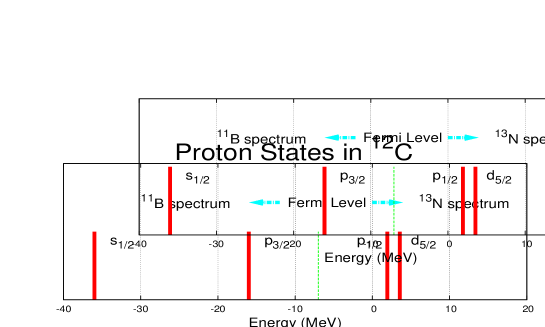
Figure 7: Single particle energies of ¹²C. The particle states (above the Fermi level) $1p_{1/2}$, and $1d_{5/2}$ are the lowest states in ¹³N, while the hole states (below the Fermi level) $1s_{1/2}$, and $1p_{3/2}$ are the lowest levels (in inverted order) in ¹¹B.

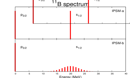
Figure 8: Schematical representation of the $1s_{1/2}$, and $1p_{3/2}$ levels in ¹¹B within the models IPSM-a (upper panel), and IPSM-b (lower panel). Due to the coupling between hole and particle states, the deeply bound hole states acquire a width and is treated as continuum state in the IPSM-b model.

Before proceeding a few words should be said on the s.p.e. of the emitted nucleon $N=n,p$ in the two-nucleon decay $\Lambda n\rightarrow nN$, which in the first section has been denoted by $\varepsilon_{N}^{\downarrow}$. Let us consider the decay ${}^{12}_{\Lambda}$C$\rightarrow^{10}$B$+\Lambda+p$, as one example. The s.p.e. of ¹²C are displayed in Fig. 7. In the pure IPSM the particle states (above the Fermi level) $1p_{1/2}$, and $1d_{5/2}$ are the lowest states in ¹³N, while the hole states (below the Fermi level) $1s_{1/2}$, and $1p_{3/2}$ are the lowest levels (in inverted order) in ¹¹B, as illustrated in the upper panel in Fig. 8. The $1s_{1/2}$ orbital is separated from the $1p_{3/2}$ state by approximately $23$ MeV, which is enough to break the $10$ particle system of ¹⁰B, where the energy of the last excited state amounts to $\sim 16.5$ MeV. In fact, a single-particle state $|j_{N}\rangle$ that is deeply bound in the hypernucleus, after the NMWD can become a highly excited hole-state $|j^{-1}_{N}\rangle$ in the continuum of the residual nucleus. There it suddenly mixes up with more complicated configurations (2h1p, 3h2p, …excitations, collective states, etc.) spreading its strength in a relatively wide energy interval Ma85 , as schematically represented in the lower panel in in Fig. 8. Although the detailed structure and fragmentation of hole states are still not well known, the exclusive knockout reactions provide a wealth of information on the structure of single-nucleon states of nuclei. Excitation energies and widths of proton-hole states were systematically measured with quasifree $(p,2p)$ and $(e,e^{\prime}p)$ reactions, which revealed the existence of inner orbital shells in nuclei Ja73 ; Fr84 ; Be85 ; Le94 ; Ya96 ; Ya01 ; Yo03 ; Ya04 ; Ko06 .

Therefore, the following two approaches for the final states $|\alpha_{N}J_{F}\rangle$ will be examined within the IPSM:

4.1 IPSM-a

Here, we completely ignore the residual interaction and, consequently, the only states $|\alpha_{N}J_{F}\rangle$ giving a nonzero result in Eq. (44) and therefore contributing to Eq. (19) are those obtained by the weak coupling, and properly antisymmetrizing, of the one hole (1h) states $|j^{-1}_{N}\rangle$ to the core ground-state $|J_{C}\rangle$. Then,

$$|\alpha_{N}J_{F}\rangle\mapsto|j_{N}J_{F}\rangle\equiv|(J_{C},j^{-1}_{N})J_{F}\rangle\,,\quad\mathrm{and}\quad E_{\alpha_{N}J_{F}}\mapsto E_{j_{N}}\equiv E_{C}-\epsilon_{j_{N}}\,,$$ (44)

where $\epsilon_{j_{N}}$ is the single-particle energy of state $j_{N}$, and the liberated energy in Eq. (40) becomes

$$\Delta_{\alpha_{N}J_{F}}\mapsto\Delta_{j_{N}}=\Delta+\epsilon_{j_{\Lambda}}+\epsilon_{j_{N}}.$$ (45)

As an illustration, in the case of ${}^{28}_{\Lambda}$Si the model space contains four single-particle states, both for protons and for neutrons ($\mathrm{n}_{p}=\mathrm{n}_{n}=4$), namely, $1s_{1/2}$, $1p_{3/2}$, $1p_{1/2}$ and $1d_{5/2}$. Thus, if the core state is $|J_{C}\rangle=|1d_{5/2}n^{-1}\rangle$, the final states $|(J_{C},j^{-1}_{N})J_{F}\rangle$ are constructed by creating two holes in the ²⁸Si nucleus, and read:

$$\begin{array}[]{ll}\underline{{}_{\Lambda}^{28}{\rm Si}\rightarrow nn+{{}^{26}{\rm Si}}}&\underline{{}_{\Lambda}^{28}{\rm Si}\rightarrow np+{{}^{26}{\rm Al}}}\\ \\ |(1d_{5/2}n^{-1})^{2};0,2,4\rangle&|(1d_{5/2}n^{-1}1d_{5/2}p^{-1});0,1,2,3,4,5\rangle\\ |1d_{5/2}n^{-1}1s_{1/2}n^{-1};2,3\rangle&|1d_{5/2}n^{-1}1s_{1/2}p^{-1};2,3\rangle\\ |1d_{5/2}n^{-1}1p_{1/2}n^{-1};2,3\rangle&|1d_{5/2}n^{-1}1p_{1/2}p^{-1};2,3\rangle\\ |1d_{5/2}n^{-1}1p_{3/2}n^{-1};1,2,3,4\rangle&|1d_{5/2}n^{-1}1p_{3/2}p^{-1};1,2,3,4\rangle.\end{array}$$ (52)

After making the substitution (45) in Eqs. (12)-(39) one can perform the summation on ${\alpha_{N}J_{F}}$ for each single-particle state $j_{N}$, as done in (Kr03, , Eqs. (11), (12), (13)), and do

$$\mathcal{F}_{\alpha_{N}J_{F}}(pP)\mapsto\mathcal{F}_{j_{N}}(pP) = \sum_{J=|j_{N}-1/2|}^{J=j_{N}+1/2}F^{j}_{NJ}\sum_{SlL\lambda T}|{{\cal M}}(plPL\lambda SJ\mathsf{T};{j_{\Lambda}j_{N}J\mathsf{t}_{\Lambda N}})|^{2},$$

with the $F^{j}_{NJ}$ are defined as

$$F^{j}_{NJ} = \hat{J_{I}}^{-2}\sum_{J_{F}}|\langle J_{I}||\left(a_{j_{N}}^{\dagger}a_{j_{\Lambda}}^{\dagger}\right)_{J}||J_{F}\rangle|^{2}$$ (56)

$$= \hat{J}^{2}\sum_{J_{F}}\left\{\negthinspace\begin{array}[]{ccc}J_{C}&J_{I}&j_{\Lambda}\\ J&j_{N}&J_{F}\end{array}\right\}^{2}|\langle J_{C}||a_{j_{N}}^{\dagger}||J_{F}\rangle|^{2}.$$

The general formula (17), (22), (26), and (34), read now

$$\Gamma_{N} = \frac{16M^{3}}{\pi}\left(\frac{A-2}{A}\right)^{3/2}\int_{0}^{\Delta}d{\epsilon}_{P}\sum_{j_{N}}\sqrt{{\epsilon}_{P}(\Delta_{j_{N}}-{\epsilon}_{P})}\mathcal{F}_{j_{N}}(pP),$$ (57)

$$\Gamma_{N}=\frac{4M^{3}}{\pi}\sqrt{A(A-2)^{3}}\int_{0}^{\Delta}dE_{nN}\sum_{j_{N}}\sqrt{(\Delta_{j_{N}}-E_{nN})(E_{nN}-\Delta_{j_{N}}^{\prime})}\mathcal{F}_{j_{N}}(pP),$$ (58)

$$\Gamma_{N} = \frac{2M}{\pi}\sqrt{\frac{A-2}{A}}\int_{0}^{P_{\Delta}}dP\sum_{j_{N}}P^{2}\sqrt{P^{2}_{\Delta_{j_{N}}}-P^{2}}\mathcal{F}_{j_{N}}(pP),$$ (59)

and

$$\Gamma_{N} = (A-2)\frac{8M^{3}}{\pi}\sum_{j_{N}}\int_{-1}^{+1}d\cos\theta_{nN}\int_{0}^{E_{j_{N}}^{max}}dE_{N}\sqrt{\frac{E_{N}}{E^{\prime}}}E_{n}\mathcal{F}_{j_{N}}(pP).$$ (60)

The meaning of all other quantities is self-evident from the initial expresions.

4.2 IPSM-b

Formally, one starts from the unperturbed basis $|i_{N}J_{F}\rangle_{0}$ with $i_{N}=1,2,\dots\mathrm{n}_{N},\mathrm{n}_{N}+1,\dots$, where for $i_{N}\leq\mathrm{n}_{N}$ we have the same simple doorway states $|j_{N}J_{F}\rangle$ in Eq. (45) (listed in Eq. (52) for ${}^{28}_{\Lambda}$Si), while for $i_{N}\geq\mathrm{n}_{N}+1$ we have more complicated bound configurations (such as $3h1p$, $4h2p$, …in the case of ${}^{28}_{\Lambda}$Si) as well as those including unbound single-particle states in the continuum. As in Ref. Ma85 , the perturbed eigenkets $|\alpha_{N}J_{F}\rangle$ and eigenvalues $E_{\alpha_{N}J_{F}}$ are obtained by diagonalizing the matrix ${}_{0}\langle i_{N}J_{F}|H|i^{\prime}_{N}J_{F}\rangle_{0}$ of the exact Hamiltonian $H$:

$$\langle\alpha_{N}J_{F}|H|\alpha^{\prime}_{N}J_{F}\rangle=E_{\alpha_{N}J_{F}}\,\delta_{\alpha_{N}\alpha^{\prime}_{N}}$$ (61)

with

$$|\alpha_{N}J_{F}\rangle = \sum_{i_{N}=1}^{\infty}C_{i_{N}}^{\alpha_{N}J_{F}}|i_{N}J_{F}\rangle_{0}$$ (62)

$$= \sum_{j_{N}}C_{j_{N}}^{\alpha_{N}J_{F}}|j_{N}J_{F}\rangle+\sum_{i_{N}=\mathrm{n}_{N}+1}^{\infty}C_{i_{N}}^{\alpha_{N}J_{F}}|i_{N}J_{F}\rangle_{0}\,.$$

It is easy to see that only the ket $|j_{N}J_{F}\rangle$ in the expansion (62) will contribute to the matrix element $\langle J_{C}||a^{\dagger}_{j_{N}}||\alpha_{N}J_{F}\rangle$ in Eq. (13). Therefore, the Eq. (17) takes the form

$$\Gamma_{N} = \frac{16M^{3}}{\pi}\left(\frac{A-2}{A}\right)^{3/2}\int_{0}^{\Delta}d{\epsilon}_{P}\sum_{j_{N}\alpha_{N}J_{F}}|C_{j_{N}}^{\alpha_{N}J_{F}}|^{2}\sqrt{{\epsilon}_{P}(\Delta_{\alpha_{N}J_{F}}-{\epsilon}_{P})}\mathcal{F}_{j_{N}J_{F}}(pP),$$

where

$$\mathcal{F}_{j_{N}J_{F}}(pP) = \hat{J}_{I}^{-2}\sum_{lL\lambda SJT}\left|\mathcal{M}(pPlL\lambda SJT;j_{N})\langle J_{I}||\left(a^{\dagger}_{j_{N}}a^{\dagger}_{j_{\Lambda}}\right)_{J}||j_{N}J_{F}\rangle\right|^{2}\,.$$ (64)

To evaluate the amplitudes $C_{j_{N}}^{\alpha_{N}J_{F}}$ one would have to choose the appropriate Hamiltonian $H$ and the unperturbed basis $|i_{N}J_{F}\rangle_{0}$, and solve the eigenvalue problem (61). We will not do this here. Instead, we make a phenomenological estimate Ba08 . First, because of the high density of states, we will convert the discrete energies $\Delta_{\alpha_{N}J_{F}}$ into the continuous variable $\varepsilon$, and the discrete sum on ${\alpha_{N}}$ into an integral on $\varepsilon$, i.e.,

$$\Delta_{\alpha_{N}J_{F}}\to\varepsilon\,,\quad\sum_{\alpha_{N}J_{F}}|C_{j_{N}}^{\alpha_{N}J_{F}}|^{2}\to\sum_{J_{F}}\int_{-\infty}^{\infty}|C_{j_{N}J_{F}}(\varepsilon)|^{2}\rho_{J_{F}}(\varepsilon)d\varepsilon\,,$$ (65)

where $\rho_{J_{F}}(\varepsilon)$ is the density of perturbed states with angular momentum $J_{F}$. In this way the Eq. (LABEL:4.14) becomes

$$\Gamma_{N} = \frac{16M^{3}}{\pi}\left(\frac{A-2}{A}\right)^{3/2}\int_{0}^{\Delta}d{\epsilon}_{P}\sum_{j_{N}J_{F}}\int_{-\infty}^{\infty}d\varepsilon\mathrm{P}_{j_{N}J_{F}}(\varepsilon){\epsilon}_{P}\sqrt{{\epsilon}_{P}(\varepsilon-{\epsilon}_{P})}\mathcal{F}_{j_{N}J_{F}}(pP),$$

where

$$\mathrm{P}_{j_{N}J_{F}}(\varepsilon)=|C_{j_{N}J_{F}}(\varepsilon)|^{2}\rho_{J_{F}}(\varepsilon)$$ (67)

is called the strength function Ma85 ; Fraz96 ; Sarg00 and represents the probability of finding the configuration $|j_{N}J_{F}\rangle\equiv|(J_{C},j_{N}^{-1})J_{F}\rangle$ per unit energy interval. Moreover, the Eq. (20) is substituted by

$$P=2\sqrt{\frac{A-2}{A}M{\epsilon}_{P}},\hskip 14.22636ptp=\sqrt{M(\varepsilon-{\epsilon}_{P})},$$ (68)

and the condition $\varepsilon\geq{\epsilon}_{P}$ has to be fulfilled throughout the $\varepsilon$ integration. It is convenient to introduce the averaged strength function

$$\mathrm{P}_{j_{N}}(\varepsilon)=\frac{1}{\dim(j_{N}J_{C})}\sum_{J_{F}=|J_{C}-j_{N}|}^{J_{C}+j_{N}}\mathrm{P}_{j_{N}J_{F}}(\varepsilon)\,,$$ (69)

where

$$\dim(j_{N}J_{C})=\left\{\begin{array}[]{lcl}2j_{N}+1&\mathrm{for}&j_{N}\leq J_{C}\,,\\ 2J_{C}+1&\mathrm{for}&J_{C}<j_{N}\,.\end{array}\right.$$ (70)

This allows to simplify Eq. (LABEL:4.17) by making the approximation $\mathrm{P}_{j_{N}J_{F}}(\varepsilon)\approx\mathrm{P}_{j_{N}}(\varepsilon)$ to get

$$\Gamma_{N} = \frac{16M^{3}}{\pi}\left(\frac{A-2}{A}\right)^{3/2}\int_{0}^{\Delta}d{\epsilon}_{P}\sum_{j_{N}}\int_{-\infty}^{\infty}d\varepsilon\mathrm{P}_{j_{N}J_{F}}(\varepsilon){\epsilon}_{P}\sqrt{{\epsilon}_{P}(\varepsilon-{\epsilon}_{P})}\mathcal{F}_{j_{N}}(pP).$$

The IPSM-a results would be recovered if one made the further approximation

$${\rm P}_{j_{N}}(\varepsilon)=\delta(\varepsilon-\Delta_{j_{N}}).$$ (72)

Here, in IPSM-b, the $\delta$-functions (72) will be used for the strictly stationary states, while for the fragmented hole states we will use Breit-Wigner distributions,

$${\rm P}_{j_{N}}(\varepsilon)=\frac{2\gamma_{j_{N}}}{\pi}\frac{1}{\gamma_{j_{N}}^{2}+4(\varepsilon-\Delta_{j_{N}})^{2}},\hskip 28.45274pt\int^{\infty}_{-\infty}{\rm P}_{j_{N}}(\varepsilon)d\varepsilon=1,$$ (73)

where $\gamma_{j_{N}}$ are the widths of the resonance centroids at energies $\Delta_{j_{N}}$ (see (Ma85, , Eq.(2.11.22))). One proceeds similarly with the Eqs. (22), (26), and (34). It turns out that the expressions within the IPSM-b can be obtained from those of IPSM-a through the replacements:

$$\Delta_{j_{N}}\mapsto\varepsilon,\hskip 14.22636pt\mbox{and}\hskip 14.22636pt\sum_{j_{N}}\cdots\mapsto\sum_{j_{N}}\int_{-\infty}^{+\infty}d\varepsilon{\rm P}_{j_{N}}(\varepsilon)\cdots.$$ (74)

To evaluate the transition rates $\Gamma_{N}$ we need to know the spectroscopic factors $F^{j}_{NJ}$ given by (56), which depend on the angular momenta $J_{C}$ and $J_{I}$, experimental values of which are given in Table 1. It is also necessary to choose between the $jj$ and $LS$ couplings. As in the previous work Kr03 (see Table I) we used here the $jj$-coupling, which is extensively used in nuclear physics in view of large spin-orbit splitting. In fact, the experimental $p_{1/2}-p_{3/2}$ energy difference is $\approx 6$ MeV around ¹⁶O. The resulting spectroscopic factors are shown in Table 2.

Nucleus	${}^{3}_{\Lambda}$H	${}^{4}_{\Lambda}$He	${}^{4}_{\Lambda}$H	${}^{5}_{\Lambda}$He	${}^{7}_{\Lambda}$Li	${}^{9}_{\Lambda}$Be	${}^{11}_{\Lambda}$B	${}^{12}_{\Lambda}$C	${}^{13}_{\Lambda}$C	${}^{15}_{\Lambda}$N	${}^{16}_{\Lambda}$O	${}^{17}_{\Lambda}$O	${}^{28}_{\Lambda}$Si
$J_{C}$	$1$	$1/2$	$1/2$	$0$	$1$	$0$	$3$	$3/2$	$0$	$1$	$1/2$	$0$	$5/2$
$J_{I}$	$1/2$	$0$	$1$	$1/2$	$1/2$	$1/2$	$5/2$	$1$	$1/2$	$3/2$	$1$	$1/2$	$2$

Table 1: Experimental values of core spin $J_{C}$, and initial spin $J_{C}$ for several $\Lambda$-hypernuclei.

$j$	$NJ$	${}^{3}_{\Lambda}$H	${}^{4}_{\Lambda}$He	${}^{4}_{\Lambda}$H	${}^{5}_{\Lambda}$He	${}^{7}_{\Lambda}$Li	${}^{9}_{\Lambda}$Be	${}^{11}_{\Lambda}$B	${}^{12}_{\Lambda}$C	${}^{13}_{\Lambda}$C	${}^{15}_{\Lambda}$N	${}^{16}_{\Lambda}$O	${}^{17}_{\Lambda}$O	${}^{28}_{\Lambda}$Si
s1/2	$n0$	$3/2$	$2$	$1$	$1$	$1$	$1$	$1$	$1$	$1$	$1$	$1$	$1$	$1$
	$n1$	$1/2$	$0$	$3$	$3$	$3$	$3$	$3$	$3$	$3$	$3$	$3$	$3$	$3$
	$p0$	$3/2$	$1$	$2$	$1$	$1$	$1$	$1$	$1$	$1$	$1$	$1$	$1$	$1$
	$p1$	$1/2$	$3$	$0$	$3$	$3$	$3$	$3$	$3$	$3$	$3$	$3$	$3$	$3$
$p_{3/2}$	$n1$	$-$	$-$	$-$	$-$	$5/2$	$3$	$13/2$	$7$	$6$	$6$	$6$	$6$	$6$
	$n2$	$-$	$-$	$-$	$-$	$3/2$	$5$	$11/2$	$5$	$10$	$10$	$10$	$10$	$10$
	$p1$	$-$	$-$	$-$	$-$	$5/2$	$3$	$13/2$	$6$	$6$	$6$	$6$	$6$	$6$
	$p2$	$-$	$-$	$-$	$-$	$3/2$	$5$	$11/2$	$10$	$10$	$10$	$10$	$10$	$10$
$p_{1/2}$	$n0$	$-$	$-$	$-$	$-$	$-$	$-$	$-$	$-$	$-$	$0$	$0$	$1$	$1$
	$n1$	$-$	$-$	$-$	$-$	$-$	$-$	$-$	$-$	$-$	$2$	$2$	$3$	$1$
	$p0$	$-$	$-$	$-$	$-$	$-$	$-$	$-$	$-$	$-$	$0$	$1$	$1$	$1$
	$p1$	$-$	$-$	$-$	$-$	$-$	$-$	$-$	$-$	$-$	$2$	$3$	$3$	$3$
$d_{5/2}$	$n2$	$-$	$-$	$-$	$-$	$-$	$-$	$-$	$-$	$-$	$-$	$-$	$-$	$16$
	$n3$	$-$	$-$	$-$	$-$	$-$	$-$	$-$	$-$	$-$	$-$	$-$	$-$	$14$
	$p2$	$-$	$-$	$-$	$-$	$-$	$-$	$-$	$-$	$-$	$-$	$-$	$-$	$15$
	$p3$	$-$	$-$	$-$	$-$	$-$	$-$	$-$	$-$	$-$	$-$	$-$	$-$	$21$

Table 2: Spectroscopic factors $F^{j}_{NJ}$ multiplied by $2j+1$.

5 NMWD Spectra

The transition probability densities $S_{nN}({\epsilon}_{P})$, $S_{nN}(E_{nN})$ $S_{nN}(P)$, $S_{nN}(\cos\theta_{nN})$, and $S_{N}(E_{N})$, can now be obtained by performing derivatives on ${\epsilon}_{P}$, $E_{nN}$, $P$, $E_{N}$, and $\cos\theta_{nN}$ in the appropriate equation for $\Gamma_{N}$, namely, Eqs. (57),(58),(59), (60), and (60), respectively.

5.1 Effects of the deeply bound hole states

In Ref. Ba08 we have studied the effects of the deeply bound hole states on the correlation spectra $S_{nN}(E_{nN})$ of several hypernuclei. The Fig. 9 shows the normalized energy spectra $S_{np}(E)/\Gamma_{p}$ for ${}^{4}_{\Lambda}$He, ${}^{5}_{\Lambda}$He, ${}^{12}_{\Lambda}$C, ${}^{16}_{\Lambda}$O, and ${}^{28}_{\Lambda}$Si hypernuclei, evaluated within the full OMEP, that comprises the ($\pi,\eta,K,\rho,\omega,K^{*}$) mesons. Quite similar results are obtained for the nn pair, i.e., for $S_{nn}(E)/\Gamma_{n}$. The s.p.e.’s for the strictly stationary hole states have been taken from Wapstra and Gove’s compilation Wa71 , and those of the quasi-stationary ones have been estimated from the studies of the quasi-free scattering processes $(p,2p)$ and $(e,e^{\prime}p)$ Ja73 ; Fr84 ; Be85 ; Le94 ; Ya96 ; Ya01 ; Yo03 ; Ya04 ; Ko06 .

Figure 9: (Color online) Normalized energy spectra $S_{np}(E)/\Gamma_{p}$ for ${}^{4}_{\Lambda}$He, ${}^{5}_{\Lambda}$He, ${}^{12}_{\Lambda}$C, ${}^{16}_{\Lambda}$O, and ${}^{28}_{\Lambda}$Si hypernuclei for the full OMEP obtained within the approaches IPSM-a (upper panel) and IPSM-b (lower panel). For the $s$-shell hypernuclei, only the IPSM-a approach has been used.

The two IPSM approaches exhibit some quite important differences:

• IPSM-a: The spectra cover the energy region $110$ MeV $<E<170$ MeV and contain one or more peaks, the number of which is equal to the number of shell-model orbitals $1s_{1/2},1p_{3/2},1p_{1/2},1d_{5/2},2s_{1/2},1d_{3/2}\cdots$ that are either fully or partly occupied in $|J_{C}\rangle$. Before including the recoil, all these peaks would be just spikes at the liberated energies $\Delta_{j_{N}}$, as can be seen from (15) setting $E_{r}=0$. With the recoil effect, they behave as

  $$S_{nN}(E\cong\Delta_{j_{N}})\sim\sqrt{(\Delta_{j_{N}}-E)(E-\Delta^{\prime}_{j_{N}})}e^{-M(A-2)(\Delta_{j_{N}}-E)b^{2}},$$ (75)

  and develop rather narrow widths $\sim[b^{2}M(A-2)]^{-1}$, where $b$ is the harmonic oscillator size parameter, which has been taken from Ref. It02 . These widths go from $\cong 3$ MeV for ${}^{28}_{\Lambda}$Si to $\cong 20$ MeV for ${}^{4}_{\Lambda}$He, as indicated in the upper panels of the just mentioned figures.

• IPSM-b: In the lower panels of the same figures are shown the results obtained when the recoil is convoluted with the Breit-Wigner distributions (73) for the strength functions of the fragmented deep hole states. The widths $\gamma_{j_{N}}$ have been estimated from Refs. Ja73 ; Fr84 ; Be85 ; Ma85 ; Le94 ; Ya96 ; Ya01 ; Yo03 ; Ya04 ; Ko06 , and in particular from (Ja73, , Fig.11) and (Ya96, , Table 1), with results: $\gamma_{{1s_{1/2}}}=9$ MeV in ${}^{12}_{\Lambda}$C, $\gamma_{{1s_{1/2}}}=14$ MeV and $\gamma_{{1p_{3/2}}}=3$ MeV in ${}^{16}_{\Lambda}$O, and $\gamma_{{1s_{1/2}}}=16$ MeV and $\gamma_{{1p_{3/2}}}=\gamma_{{1p_{1/2}}}=5$ MeV in ${}^{28}_{\Lambda}$Si, both for protons and neutrons. One sees that, except for the ground states, the narrow peaks engendered by the recoil effect become now pretty wide bumps.

We feel that the above rather rudimentary parameterization could be realistic enough for a qualitative discussion of the kinetic energy sum spectra. A more accurate model should be probably necessary for a full quantitative study and comparison with data.

5.2 Interpretation of BNL experiment E788 on ${}^{4}_{\Lambda}$He

Particularly interesting is the Brookhaven National Laboratory experiment E788 on ${}^{4}_{\Lambda}$He, performed by Parker et al.  Par07 , which highlighted that the effects of the Final State Interactions (FSI) on the one-nucleon induced decay, as well as the contributions of the two-nucleon induced decays, $\Lambda NN\rightarrow nNN$, could be very small in this case, if any.

Therefore one might hope that the IPSM could be an adequate framework to account for the NMWD spectra of this hypernucleus. This has been done in Ref. Bau09 by employing the $\pi+K$ exchange potential, with soft cutoffs ($\Lambda_{\pi}=0.7$ GeV and $\Lambda_{K}=0.9$ GeV), which is capable of accounting for the experimental values related to $\Gamma_{p}$ and $\Gamma_{n}$ in all three ${}^{4}_{\Lambda}$H, ${}^{4}_{\Lambda}$He, and ${}^{5}_{\Lambda}$He hypernuclei Bau09 . It is labelled as SPKE model and is not very different from the PKE model used by Sasaki et al.  Sa02 .

The transition probability densities $S_{N}(E)$, $S_{nN}(E)$, and $S_{nN}(\cos\theta)$ contain the same dynamics, but involve different phase-space kinematics for each case. In particular, the proton spectrum $S_{p}(E)$ is related with the expected number of protons $d{\rm N}_{p}(E)$ detected within the energy interval $dE$ through the relation

$$\frac{d{\rm N}_{p}(E)}{dE}=C_{p}(E)S_{p}(E),$$ (76)

where $C_{p}(E)$ depends on the proton experimental environment and includes all quantities and effects not considered in $S_{p}(E)$, such as the number of produced hypernuclei, the detection efficiency and acceptance, etc. In experiment E788, after correction for acceptance, the remaining $C_{p}(E)$ factor is approximately energy-independent in the region beyond the detection threshold, $E^{0}_{p}$ Par08 . In what follows, we will always compare our predictions with the experimental spectra that have been corrected for acceptance and take into account the detection threshold. Thus we can write, for the expected number of detected protons above this threshold,

$$\bar{{\rm N}}_{p}=\int_{E_{p}^{0}}^{E_{p}^{max}}\frac{d{\rm N}_{p}(E)}{dE}dE=\bar{C}_{p}\int_{E_{p}^{0}}^{E_{p}^{max}}S_{p}(E)dE=\bar{C}_{p}\bar{\Gamma}_{p}.$$ (77)

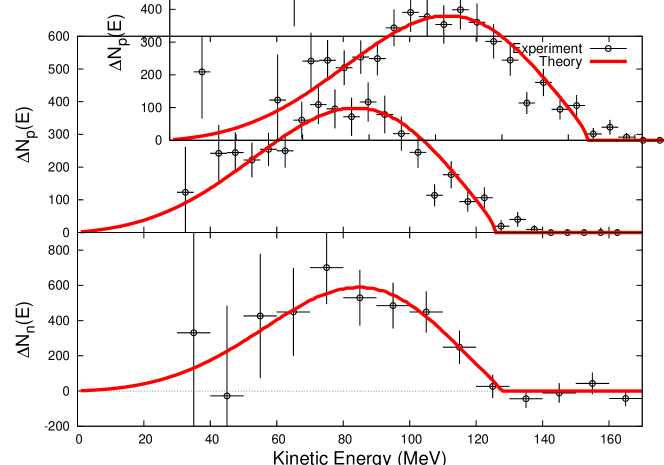
Figure 10: Comparison between the experimental and theoretical kinetic energy spectra for protons (upper panel) and neutrons (lower panel). The data are acceptance corrected Par08 , and the calculated results are obtained from Eqs. (80) and (81).

This allows us to rewrite (76) in the form

$$\frac{d{\rm N}_{p}(E)}{dE}={\bar{{\rm N}}_{p}}\frac{S_{p}(E)}{\bar{\Gamma}_{p}}\qquad(E>E_{p}^{0}).$$ (78)

The spectrum $S_{p}(E)$ is normalized to the experimental one by replacing $\bar{{\rm N}}_{p}$ in (78) with the acceptance-corrected number of actually observed protons,

$$\bar{{\rm N}}_{p}^{exp}=\sum_{i=1}^{m}\Delta{\rm N}_{p}^{exp}(E_{i}),$$ (79)

where $\Delta{\rm N}_{p}^{exp}(E_{i})$ is the acceptance-corrected number of protons measured at energy $E_{i}$ within a fixed energy bin $\Delta E_{p}$, and $m$ is the number of bins beyond the detection threshold. Thus, the quantity that we have to confront with data is

$$\Delta{\rm N}_{p}(E)={\bar{\rm N}}_{p}^{exp}\Delta E_{p}\frac{S_{p}(E)}{\bar{\Gamma}_{p}},$$ (80)

where the barred symbols ($\bar{\rm N}_{p}^{exp}=4546$, and $\bar{\Gamma}_{p}=0.168$) indicate that the proton threshold $E^{0}_{p}=40$ MeV Par08 has been considered in the numerical evaluation of the corresponding quantities. In contrast to $\Delta{\rm N}_{p}^{exp}(E_{i})$, $\Delta{\rm N}_{p}(E)$ is a continuous function of $E$.

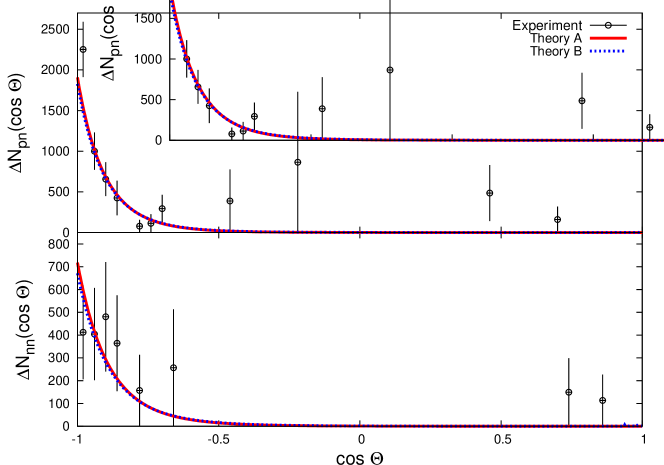
Figure 11: Comparison between experimental opening angle correlations for proton-neutron (upper panel) and neutron-neutron (lower panel) pairs. The data $\widetilde{\Delta{\rm N}}_{nN}^{exp}(\cos\theta_{i})$ are acceptance corrected and do not contain events with $E_{N}<30$ MeV Par08 . The theoretical results are obtained from Eq. (83), with $\widehat{{\rm N}}_{nN}^{exp}$ only containing events with $\cos\theta_{nN}<-0.5$. Two cases are presented: 1) Theory A, where both the angular and the single kinetic energy cuts are taken into account, and 2) Theory B, where the cuts are not considered in the calculations.

As the one-proton (one-neutron) induced decay prompts the emission of an $np$ ($nn$) pair, one has in the same way for the one-neutron spectrum

$$\Delta{\rm N}_{n}(E)={\bar{\rm N}}_{n}^{exp}\Delta E_{n}\frac{S_{p}(E)+2S_{n}(E)}{\bar{\Gamma}_{p}+2\bar{\Gamma}_{n}}.$$ (81)

Here, ${\bar{\rm N}}_{n}^{exp}=3565$, and $\bar{\Gamma}_{p}+2\bar{\Gamma}_{n}=0.198$ have been evaluated with a neutron threshold of $30$ MeV Par08 . In Fig. 10, our results are compared with the measurements of Parker et al.  Par07 . A similar, but somewhat different, procedure is followed for the coincidence spectra. The main difference arises from the fact that the angular-correlation spectra, $\Delta{\rm N}_{nN}^{exp}(\cos\theta_{i})$, as well as the kinetic energy sum data, $\Delta{\rm N}_{nN}^{exp}(E_{i})$, besides being acceptance-corrected, were measured with detection thresholds of $30$ MeV for both neutrons and protons. More, in the selection of the kinetic energy sum data it was also applied an angular cut of $\cos\theta_{nN}<-0.5$. In order to make the presentation simple, the observables that comprise only the energy cuts, and those that include both the energy and the angular cuts, will be indicated by putting, respectively, a tilde and a hat over the corresponding symbols.

Thus, the number of $nN$ pairs measured in coincidence can be expressed as

$$\widehat{{\rm N}}_{nN}^{exp}=\sum_{i=1}^{k}\widetilde{\Delta{\rm N}}_{nN}^{exp}(\cos\theta_{i})=\sum_{i=1}^{l}{\widehat{\Delta{\rm N}}}_{nN}^{exp}(E_{i}),$$ (82)

where the angular bins with $\cos\theta_{i}>-0.5$ are excluded from the first summation. The $\widetilde{\Delta{\rm N}}_{nN}^{exp}(\cos\theta_{i})$ and ${\widehat{\Delta{\rm N}}}_{nN}^{exp}(E_{i})$ data should be compared, respectively, with

$$\widetilde{\Delta{\rm N}}_{nN}(\cos\theta)=\widehat{{\rm N}}_{nN}^{exp}\Delta\cos\theta_{nN}\frac{\widetilde{S}_{nN}(\cos\theta)}{\widehat{{\Gamma}}_{N}},$$ (83)

and

$$\widehat{\Delta{\rm N}}_{nN}(E)=\widehat{{\rm N}}_{nN}^{exp}\Delta E_{nN}\frac{\widehat{S}_{nN}(E)}{\widehat{{\Gamma}}_{N}}.$$ (84)

Here, from Ref. Par08 $\widehat{{\rm N}}_{np}^{exp}=4821$, $\widehat{{\rm N}}_{nn}^{exp}=2075$, $\Delta\cos\theta_{nN}=0.04$ and $\Delta E_{nN}=10$ MeV, while $\widehat{\Gamma}_{p}=0.1709$ and $\widehat{\Gamma}_{n}=0.0113$. These results (Theory A) are compared with the E788 data in Figs. 11 and 12. For completeness, in the same figures are also shown the results for $\widetilde{S}_{nN}(\cos\theta)\rightarrow{S}_{nN}(\cos\theta)$, $\widehat{S}_{nN}(E)\rightarrow{S}_{nN}(E)$ and $\widehat{\Gamma}_{N}\rightarrow{\Gamma}_{N}$, i.e., when no energy and angular cuts are considered in the theoretical evaluation, and ${\Gamma}_{p}=0.1793$ and ${\Gamma}_{n}=0.0122$ (Theory B).

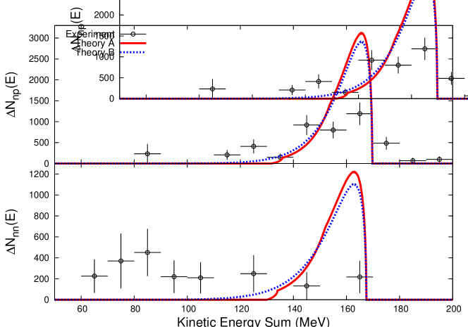
Figure 12: Comparison between experimental kinetic energy sum spectra for proton-neutron (upper panel) and neutron-neutron (lower panel) pairs. The data $\widehat{\Delta{\rm N}}_{nN}^{exp}(E_{i})$ are acceptance corrected and only contain events with $E_{N}>30$ MeV and $\cos\theta_{nN}<-0.5$ Par08 . The theoretical results are obtained from Eq. (84), and two cases are shown: 1) Theory A, where both cuts are taken into account, and 2) Theory B, where the cuts are not considered in the calculations.

We conclude that the overall agreement between the measurements of Parker et al.  Par07 and the present calculations is quite satisfactory, although we are not considering contributions coming from the two-body induced decay, $\Lambda NN\rightarrow nNN$, nor from the rescattering of the nucleons produced in the one-body induced decay, $\Lambda N\rightarrow nN$. However, before ending the discussion we would like to point out that:

1. As expected, the theoretical spectrum $\Delta{\rm N}_{p}(E)$, shown in the upper panel of Fig. 10, is peaked around $85$ MeV, corresponding to the half of the $Q$-value $\Delta_{p}=170$ MeV. Yet, as the single kinetic energy reaches rather abruptly its maximum value $E^{max}_{p}=127$ MeV (see Eq. (39)), the proton spectrum shape is not exactly that of a symmetric inverted bell. Something quite analogous happens in the case of neutrons, as can be seen in the lower panel of Fig. 10. The experimental data seem to behave in the same way. To some extent, this behavior of $\Delta{\rm N}_{p}(E)$ and $\Delta{\rm N}_{n}(E)$ is akin to the behavior of the $\Delta{\rm N}_{nN}(E)$, which suddenly collapse at the Q-values.

2. There are no data at really low energies for the proton case which would allow to exclude the FSI effects for sure, and the neutron data for low energies are afflicted by large error bars. However, there is no need to invoke these effects, nor those of two-nucleon induced NMWD, to explain the data, as occurs in the proton spectrum of ${}^{5}_{\Lambda}$He Ag08 . This hints at a new puzzle in the NMWD, but it is difficult to discern whether it is of experimental or theoretical nature.

3. The calculated spectra $\widetilde{\Delta{\rm N}}_{np}(\cos\theta)$ shown in the upper panel of Fig. 11, are strongly peaked near $\theta=180^{o}$, which agrees with data fairly well. However, while it is found experimentally that $28\%$ of events occur at opening angles less than $120^{o}$, theoretically we get that only $\>\raisebox{-2.15277pt}{$\stackrel{{\scriptstyle\textstyle<}}{{\sim}}$}\>2\%$ of events appear in this angular region. We find no explanation for this discrepancy. Nevertheless, the fact that not all events are concentrated at $\theta=180^{o}$, is not necessarily indicative of the contributions coming from the FSI or the $\Lambda NN\rightarrow nNN$ decay, as suggested in Ref. Par07 .

4. The calculated angular correlation $\widetilde{\Delta{\rm N}}_{nn}(\cos\theta)$, shown in the lower panel of Fig. 11, is quite similar to that of the $pn$ pair; that is, its back-to-back peak is very pronounced. This behavior is not exhibited by the experimental distribution. In addition, while $11\%$ of events are found experimentally for $\cos\theta\geq-0.5$, in the calculation only $\>\raisebox{-2.15277pt}{$\stackrel{{\scriptstyle\textstyle<}}{{\sim}}$}\>3\%$ of them appear at these angles. We feel however that, because of the poor statistics and large experimental errors, one should not attribute major importance to such disagreements.

5. Both calculated kinetic energy sum distributions $\widehat{\Delta{\rm N}}_{nN}(E)$, shown in Fig. 12, present a bump at $\approx 160$ MeV, with a width of $\approx 30$ MeV, which for protons agrees fairly well with the experiment. We would like to stress once more that the spreading in strength here is totally normal even for a purely one-nucleon induced decay. The kink at $\approx 130$ MeV within the Theory A comes from the angular cut, and from this one can realize that the ${nN}$ kinetic energy sum spectra below this energy are correlated with the angular coincidence spectra $\widetilde{\Delta{\rm N}}_{nN}(\cos\theta<-0.5)$. The bump observed in the experimental $\widehat{\Delta{\rm N}}_{nn}(E)$ spectrum at $\approx 90$ MeV is not reproduced by the theory, which may be indicative of $nn$ coincidences originated from sources other than $\Lambda n$ decays, as already suggested in Ref. Pa07 . Another source for the difference between our model calculation and the data may be traced to $np$ and $nn$ final state interactions. Whereas in the former the intensity of this interaction is reduced owing to the Coulomb repulsion felt by the proton, in the latter the two neutrons may interact strongly and thus shift the peak to lower kinetic energy sum.

In summary, to comprehend the recent measurements in ${}^{4}_{\Lambda}$He, we have outlined for the one-nucleon induced NMWD spectra a simple theoretical framework based on the IPSM. Once normalized to the transition rate, all the spectra are tailored basically by the kinematics of the corresponding phase space, depending very weakly on the dynamics governing the $\Lambda N\to nN$ transition proper. As a matter of fact, although not shown here, the normalized spectra calculated with the full PSVE model are, for all practical purposes, identical to those using the SPKE model, which we have amply discussed. In spite of the simplicity of the approach, a good agreement with data is obtained. This might indicate that, neither the FSI, nor the two-nucleon induced decay processes play a significant role in the $s$-shell, at least not for ${}^{4}_{\Lambda}$He.

6 Outlook

Before being detected the newborn nucleons in a NMWD suffer final state interactions (FSI) with the nuclear environment, and consequently their two-nucleon $\Gamma_{N}$, and three-nucleon $\Gamma_{2}$ decay rates are not observable from a quantum-mechanical point of view, as recently pointed out by Bauer and Garbarino Ba10 . These FSI give rise to emission of new secondary nucleons, that are counted by the detection systems together with the primordial ones, without being possible to distinguish ones from the others. The IPSM developed so far is a simple fully quantum-mechanical formalism for the theoretical investigation of decay rates $\Gamma_{N}$ and their spectra. It don’t describe neither the decay rate $\Gamma_{2}$ nor the FSI. Therefore, it is not surprising that this model does not reproduce well the FINUDA experiment for the ${}^{12}_{\Lambda}$C Ag08 , as shown in Fig. 13, although it reproduces well Bau09 the BNL experiment for ${}^{4}_{\Lambda}$He Par07 .

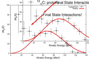
Figure 13: Comparison between the experimental Ag08 and theoretical Ba10 kinetic energy spectra for protons from ${}^{12}_{\Lambda}$C decay.

At the time being we are studying the proton kinetic energy spectra obtained in the FINUDA experiment for ${}^{5}_{\Lambda}$ He, ${}^{7}_{\Lambda}$Li, ${}^{9}_{\Lambda}$Be, ${}^{11}_{\Lambda}$B, ${}^{12}_{\Lambda}$C, ${}^{15}_{\Lambda}$C, and ${}^{16}_{\Lambda}$O Ag09 ; Ag10 . We are comparing their results with the simple IPSM, with the purpose to quantify the contributions of the FSI and the three-nucleon emission. The same is being done for the recent KEK measurments on angular correlations and kinetic energy sum of $np$ and $nn$ pairs Ok04 ; Ka06 ; Ki06 ; Ki09 , as well as the c.m. momentum spectra in ${}^{12}_{\Lambda}$C Ki09 . Later on we will include the FSI, a consistent treatment of which would require in general a genuine three-body approach for the mutual interaction of the two emitted nucleons and the residual nucleus. Presumably due to the enormous computational challenges, this has never been tackled in the past. We are also planning to extend IPSM for the evaluation of the decay rate $\Gamma_{2}$ for the emission of three primordial nucleons, which has been done so far only in the framework of the Fermi gas model Al91 ; Ra94 ; Ba03 ; Bau109 ; Bau209 .

References

- (1) E.N.E. vanDalen, and A.E.L. Dieperink, Phys.Rev. C 69, 025802 (2004).
- (2) J. Scaffner-Bielich, Nucl. Phys. A 804, 309 (2008).
- (3) C. Samanta, P. Roy Chowdhury and D.N. Basu, J. Phys. G 35, 065101 (2008).
- (4) A. Sakaguchi et al. , arXiv:0904.0298 (2009).
- (5) Q.N. Usmani and A.R. Bormer, Phys. Rev. C60, 055215 (1999).
- (6) F. Krmpotić, and D. Tadić, Braz. J. Phys. 33, 187 (2003).
- (7) A. Gal, Nucl. Phys. A828, 72 (2009).
- (8) J.B. Adams, Phys. Rev. 156, 1611 (1967).
- (9) C. Chumillas, G. Garbarino, A. Parreño, and A. Ramos, Phys. Lett. B657, 180 (2007).
- (10) J. F. Dubach, G. B. Feldman, B. R. Holstein and L. de la Torre, Ann. Phys. (N.Y.) 249, 146 (1996).
- (11) J. J. Szymanski et al., Phys. Rev. C43, 849 (1991).
- (12) H. Noumi et al., Phys. Rev. C52, 2936 (1995).
- (13) O. Hashimoto et al., Phys. Rev. Lett. 88, 042503 (2002).
- (14) E. Oset and A. Ramos, Prog. Part. Nucl. Phys. 41, 191, edited by A. Faessler, (Pergamon, 1998).
- (15) W.M. Alberico, G. Garbarino, Phys. Rep. 369 (2002) 1;
- (16) W.M. Alberico, G. Garbarino, in: T. Bressani, A. Filippi, U. Wiedner (Eds.), Hadron Physics, Proceedings of the International School of Physics Enrico Fermi , Course CLVIII, Varenna, Italy, 22 June 2 July, 2004, IOS Press, Amsterdam, 2005, p. 125, nucl-th/0410059.
- (17) A. Parreño, Lecture Notes Phys. 724 (2007) 141.
- (18) C. Chumillas, G. Garbarino, A. Parreño, and A. Ramos, Nucl. Phys. A804, 162 (2008).
- (19) C.-Y. Cheung, D. P. Heddle, and L. S. Kisslinger, Phys. Rev.C 27 (1983) 335.
- (20) K. Maltman, and M. Shmatikov, Phys. Lett. B331 (1994) 1.
- (21) T. Inoue, S. Takeuchi and M. Oka, Nucl. Phys. A597 (1996) 563.
- (22) T. Inoue, M. Oka, T. Motoba and K. Itonaga, Nucl. Phys. A633, 312 (1998).
- (23) K. Sasaki, T. Inoue, and M. Oka, Nucl.Phys. A669, 331 (2000); Erratum-ibid. A678, 455 (2000).
- (24) B. H. J. McKellar and B. F. Gibson, Phys. Rev. C30, 322 (1984).
- (25) K. Takeuchi, H. Takaki and H. Band, Prog. Theor. Phys. 73 (1985) 841.
- (26) G. Narduli, Phys. Rev. C38C 38 (1988) 832.
- (27) A. Parreño, A. Ramos and C. Bennhold, Phys. Rev. C52, R1768 (1995): C54, 1500 (E) (1996).
- (28) A. Ramos, C. Bennhold, E. van Meijgaard and B. K. Jennings, Phys. Lett. B 264 (1991) 233. (See criticism in Ref. Pa95 .)
- (29) A. Ramos, E. van Meijgaard, C. Bennhold and B. K. Jennings, Nucl. Phys. A 544 (1992) 703. (See criticism in Ref. Pa95 .)
- (30) A. Parreño, A. Ramos and E. Oset, Phys. Rev. C51, 2477 (1995).
- (31) A. Parreño, A. Ramos and C. Bennhold, Phys. Rev. C56, 339 (1997).
- (32) K. Hagino and A. Parrño, Phys. Rev. C63 (2001) 044318.
- (33) A. Parreño and A. Ramos, Phys. Rev. C65, 015204 (2001); A. Parreño, A. Ramos and C. Bennhold, Phys. Rev. C65, 015205 (2001)
- (34) C. Barbero, D. Horvat, F. Krmpotić, T. T. S. Kuo, Z. Narančić and D. Tadić, Phys. Rev. C66, 055209 (2002).
- (35) K. Sasaki, T. Inoue, M. Oka, Nucl. Phys. A 707 (2002) 477.
- (36) C. Barbero, C. De Conti, A. P. Galeão, and F. Krmpotić, Nucl. Phys. A726, 267 (2003).
- (37) E. Bauer and F. Krmpotić, Nucl. Phys. A 717, 217 (2003); A 739, 109 (2004).
- (38) C. Barbero, A. P. Galeão, and F. Krmpotić, Phys. Rev. C 72, 035210 (2005).
- (39) M. Shmatikov, Nucl. Phys. A580, 538 (1994).
- (40) K. Itonaga, T. Ueda, T. Motoba, Phys. Rev. C65, 034617 (2002).
- (41) E. Oset and L. L. Salcedo, Nucl. Phys. A 443 (1985) 704.
- (42) W. M. Alberico, A. De Pace, M. Ericson and A. Molinari, Phys. Lett. B 256 (1991) 134. (See criticism in Ref. Ra94 .)
- (43) A. Ramos, E. Oset and L. L. Salcedo, Phys. Rev. C50 (1994) 2314.
- (44) A. Ramos, M. J. Vicente-Vacas and E. Oset, Phys. Rev. C55 (1997) 735. Erratum: ibid. C66(2002) 039903.
- (45) D. Jido, E. Oset and J. E. Palomar, Nucl. Phys. A694 (2001) 525.
- (46) L. Zhou and J. Piekarewicz, Phys. Rev. C60 (1999) 024306.
- (47) K. Sasaki, T. Inoue and M. Oka, Nucl. Phys. A678, 455 (2000).
- (48) E. Oset, D. Jido and J.E. Palomar, Nucl.Phys. A691, 146 (2001); D. Jido, E. Oset and J.E. Palomar, arXiv nucl-th/0101051.
- (49) B.H. Kang, et al. , Phys. Rev. Lett. 96, 025203 (2006).
- (50) M.J. Kim, et al. , Phys. Lett. B641, 28 (2006).
- (51) J.H. Kim, et al. , Phys. Rev. C 68 (2003) 065201.
- (52) S. Okada, et al. , Phys. Lett. B 597 (2004) 249.
- (53) M. Agnello, et al. , Nucl. Phys. A 804 (2008) 151.
- (54) J. D. Parker, et al. , Phys. Rev. C 76 (2007) 035501.
- (55) S. Okada, et al. , Nucl. Phys. A 752 (2005) 169c.
- (56) H. Outa, et al. , Nucl. Phys. A 754 (2005) 157c.
- (57) H. Bhang, et al. , Eur. Phys. J. A 33 (2007) 259.
- (58) C. Barbero, A. P. Galeão, M. Hussein, and F. Krmpotić, Phys. Rev. C 78, 044312 (2008); Erratum-ibid. 059901(E).
- (59) C. Barbero, A. P. Galeão, F. Krmpotić, Phys. Rev.C 76 (2007) 0543213.
- (60) E. Bauer, A.P. Galeão, M. Hussein, F. Krmpotić, and J.D. Parker, Phys. Lett. B 674, 103 (2009).
- (61) C. Mahaux, P.E. Bortignon, R.A. Broglia, and C.H. Dasso, Phys. Rep. 120, 1 (1985).
- (62) G. Jacob and T. A. J. Maris, Rev. Mod. Phys. 45, 6 (1973).
- (63) S. Frullani, J. Mougey, Adv. Nucl. Phys. 14, 1 (1984).
- (64) S.L. Belostotskii et al. , Sov. J. Nucl. Phys. 41, 903 (1985); S.S. Volkovet al. , Sov. J. Nucl. Phys. 49, 848 (1990).
- (65) M. Leuschner et al. , Phys. Rev. C 49, 955 (1994).
- (66) T. Yamada, M. Takahashi, and K. Ikeda, Phys. Rev. C 53, 752 (1996).
- (67) T. Yamada, Nucl. Phys. A687, 297c (2001).
- (68) M. Yosoi, et al. , Phys. Lett. B551, 255 (2003).
- (69) T. Yamada, M. Yosoi, , and H. Toyokawa, Nucl. Phys. A738, 323 (2004).
- (70) K. Kobayashi, et al. , arXiv:nucl-ex/0604006.
- (71) N. Frazier, B. A. Brown, and V. Zelevinsky, Phys. Rev. C54, 1665 (1996).
- (72) A. J. Sargeant, M. S. Hussein, M. P. Pato, and M. Ueda, Phys. Rev. C61, 011302(R) (1999).
- (73) A.H. Wapstra and N. B. Gove, Nucl. Data Tables 9, 265 (1971).
- (74) J. D. Parker, private communication.
- (75) W. T. Winter, S. J. Freedman, K. E. Rehm, and J. P. Schiffer, Phys.Rev. C73 (2006) 025503.
- (76) E. Bauer, and G. Garbarino, Contribution to the 10th International Conference on Hypernuclear and Strange Particle Physics (HYP-X) Tokai, Ibaraki, Japan, September 2009, to be published in Nucl. Phys. A.
- (77) E. Bauer, A.P. Galeão, M. Hussein, and F. Krmpotić, Contribution to the NN2009 International Conference, Beijing, China, August 2009, Nucl. Phys. A834 (2010) 599c.
- (78) M. Agnello, et al. , Phys. Lett. B681 (2009) 139.
- (79) M. Agnello, et al. , Phys. Lett. B685 (2010) 247.
- (80) M.J. Kim, et al. , Phys. Rev. Lett. 103, 182502 (2009).
- (81) E. Bauer, Nucl. Phys. A818, (2009) 174.
- (82) E. Bauer, and G. Garbarino, Nucl. Phys. A828, (2009) 29.