Future constraints on variations of the fine structure constant from combined CMB and weak lensing measurements

Abstract

We forecast the ability of future CMB and galaxy lensing surveys to constrain variations of the fine structure constant. We found that lensing data, as those expected from satellite experiments as Euclid could improve the constraint from future CMB experiments leading to a $\Delta\alpha/\alpha=8\times 10^{-4}$ accuracy. A variation of the fine structure constant $\alpha$ is strongly degenerate with the Hubble constant $H_{0}$ and with inflationary parameters as the scalar spectral index $n_{s}$. These degeneracies may cause significant biases in the determination of cosmological parameters if a variation in $\alpha$ as large as $\sim 0.5\%$ is present at the epoch of recombination.

I Introduction

After the recent measurements of Cosmic Microwave Background (CMB hereafter) anisotropies, galaxy clustering and supernovae type Ia luminosity distances (see e.g. wmap7 ; sdss2 ; snalate ) cosmology has entered a ”golden age” where not only a ”standard” model of structure formation has been firmly established but also where physical assumptions not testable in laboratory can now be probed with unprecedented accuracy.

One of the most promising aspects of this new cosmological framework is indeed the possibility of testing variations of fundamental constants on scales, times and energies drastically different from those on earth.

A variation of fundamental constants in time, while certainly exciting, represents a radical departure from standard model physics. In the past years much of attention has been focused on the fine structure constant $\alpha$ mainly because of the observational indication of a smaller value in the past, at cosmological redshifts $z=0.5-3.5$, from quasar absorption systems data with $\Delta\alpha/\alpha=(-0.72\pm 0.18)\times 10^{-5}$ (webbpast ). More recently, these observations have been complemented with new data from the Very Large Telescope (VLT), covering a different region of the sky. This data shows an opposite evolution for $\alpha$, i.e. an increase respect to the local, present value, by approximately the same amount (webbrecent ) and leading to the hypothesis of an anisotropic variation in $\alpha$. While all these measurements could be affected by some hidden systematics the search for variations of the fine structure constant in the early universe is clearly a major and timely line of investigation in modern astrophysics (see e.g. uzan for a review).

CMB anisotropies have provided in the past years a powerful method to constrain variations of the fine structure constant. Since the CMB anisotropies were generated at the epoch of recombination, approximately $\sim 340.000$ years after the Big Bang, they probe the value of the fine structure constant at that time, when the universe was nearly isotropic and homogeneous. Constraints have been obtained analyzing CMB data (see e.g. avelino ; Rocha ; ichikawa ; jap ; petruta ; menegoni ; landau ; menegoniw ) with an accuracy at the level of $\sim 10-1\%$. In the most recent analysis, parametrizing a variation in the fine structure constant as $\alpha/\alpha_{0}$, where $\alpha_{0}=1/137.03599907$ is the standard (local) value and $\alpha$ is the value during the recombination, the authors of menegoni2 found the constraint $\alpha/\alpha_{0}=0.984\pm 0.005$, i.e. hinting also to a more than two standard deviation from the current value.

While the current CMB bound is considerably weaker than the observed variation from quasar spectra, the CMB recombination occurred at a time period corresponding to redshift $z\sim 1300$. It is quite possible that $\alpha$ has larger variations at higher redshifts, i.e. there is no reason for the variation to be constant in time. The CMB bound provides therefore important constraints on the running of the fine structure constant.

In the next few years, we expect a further significant improvement in the quantity and quality of cosmological data. The Planck satellite mission (see  :2006uk ), for example, will provide accurate temperature CMB maps by the end of this year. On the other hand new and larger galaxy surveys are either already operating either under study. Some of these surveys will provide new galaxy weak lensing measurements that, when combined with Planck, will drastically improve the constraints on cosmological parameters. The Euclid satellite mission euclid , selected as part of ESA Cosmic Visions programme and due for launch in 2019, probably represents the most advanced weak lensing survey that could be achieved in the current decade.

Future weak lensing surveys will measure photometric redshifts of billions of galaxies allowing the possibility a tomographic reconstruction of growth of structure as a function of time through a binning of the redshift distribution of galaxies, with a considerable improvement of cosmological information (e.g. dark energy Kitching:2007 ; on neutrinos Hannestad:2006as ; Kitching:2008dp ; the dark matter distribution as a function of redshift art:Taylor and the growth of structure art:Bacon ; art:Massey ). As far as we know, there is however still no study in the literature that considered the gain in constraining variation in fundamental constant from these surveys.

It is therefore timely to forecast the constraints on variation of the fine structure constant achievable from weak lensing data from the Euclid satellite mission. In this paper we indeed perform this kind of analysis. As expected, weak lensing probes are shown to be complementary to CMB measurements and to significantly improve the constraints on variation in the fine structure constant.

The structure of the paper is as follows. Section II contains the description of the simulated future data used in our analyses. The results from our Markov Chain Monte Carlo (MCMC) analyses are presented in Sec. III. We draw our conclusions in Sec. IV.

II Future data

In this section we describe the method adopted to simulate the future CMB and weak lensing surveys data used then to forecast the constraints on $\alpha$ and the remianing cosmological parameters.

The fiducial cosmological model assumed in producing the simulated data is the best-fit model from the WMAP seven year CMB survey (see Ref. wmap7 ). The parameters are: baryon density $\Omega_{b}h^{2}=0.02258$, cold dark mattter density $\Omega_{c}h^{2}=0.1109$, spectral index $n_{s}=0.963$, optical depth $\tau=0.088$, scalar amplitude $A_{s}=2.43\times 10^{-9}$ and Hubble constant $H_{0}=71$. For the fine structure constant we assume either the standard value $\alpha/\alpha_{0}=1$, either a small variation $\alpha/\alpha_{0}=0.996$, that we believe could be detectable with these future data.

As stated in the introduction we consider CMB data from Planck and galaxy weak lensing measurements from Euclid. For CMB data the main observables are the $C_{\ell}$ angular power spectra for temperature, polarization and cross temperature-polarization. For weak lensing data we consider the convergence power spectra $P(\ell)$ following the procedure described in fdebe011 . All spectra are generated using a modified version of the CAMB code camb taking into account the possible variation in the fine structure constant as discussed in menegoni .

II.1 CMB data

We create a full mock CMB dataset with noise properties consistent with those expected for the Planck :2006uk experiment (see Tab. 1).

Experiment	Channel	FWHM	$\Delta T/T$
Planck	70	14’	4.7
	100	10’	2.5
	143	7.1’	2.2
$f_{sky}=0.85$

Table 1: Planck-like experimental specifications. Channel frequency is given in GHz, the temperature sensitivity per pixel in $\mu K/K$, and FWHM (Full-Width at Half-Maximum) in arc-minutes. The polarization sensitivity is assumed as $\Delta E/E=\Delta B/B=\sqrt{2}\Delta T/T$.

For each channel we consider a detector noise of $w^{-1}=(\theta\sigma)^{2}$, with $\theta$ the FWHM (Full-Width at Half-Maximum) of the beam assuming a Gaussian profile and $\sigma$ the temperature sensitivity $\Delta T$ (see Tab. 1 for the polarization sensitivity). To each $C_{\ell}$ fiducial spectra we add a noise spectrum given by:

$$N_{\ell}=w^{-1}\exp(\ell(\ell+1)/\ell_{b}^{2})\,,$$ (1)

with $\ell_{b}$ given by $\ell_{b}\equiv\sqrt{8\ln 2}/\theta$.

Alongside temperature and polarization power spectra ($C_{\ell}^{TT}$, $C_{\ell}^{EE}$ and $C_{\ell}^{TE}$) we include also the the deflection power spectra $C_{\ell}^{dd}$ and $C_{\ell}^{Td}$ obtained through the quadratic estimator of the lensing deflection field $d$ presented in lensextr

$$d{(a,b)_{L}^{M}=n_{L}^{ab}\sum_{\ell\ell^{\prime}mm^{\prime}}{W{(a,b)_{\ell\ell^{\prime}L}^{mm^{\prime}M}a_{\ell}^{m}b_{\ell^{\prime}}^{m^{\prime}}}}}$$ (2)

where $n_{L}^{ab}$ is a normalization factor, $W$ is a function of the power spectra $C_{\ell}^{ab}$, which include both CMB lensing and primary anisotropy contributions, and $ab={TT,TE,EE,EB,TB}$; the $BB$ case is excluded because the method of Ref. lensextr is only valid when the lensing contribution is negligible compared to the primary anisotropy, assumption that fails for the B modes in the case of Planck.
It is possible to combine five quadratic estimators into a minimum variance estimator; the noise on the deflection field power spectrum $C_{\ell}^{dd}$ produced by this estimator can be expressed as:

$$N_{\ell}^{dd}=\frac{1}{\sum_{aa^{\prime}bb^{\prime}}{(N_{\ell}^{aba^{\prime}b^{\prime}})^{-1}}}~{}.$$ (3)

A publicly available routine (http://lesgourg.web.cern.ch/lesgourg/codes.html) allows to compute the minimum variance lensing noise for the Planck experiment. At the same URL a full-sky exact likelihood routine is available and we use this in order to analyze our forecasted datasets, which include the lensing deflection power spectrum.

II.2 Galaxy weak lensing data

We simulate future galaxy weak lensing data assuming the specifications for the Euclid weak lensing survey (see Table 2). This survey will observe about $30$ galaxies per square arcminute from redshift $z=0.5$ to $z=2$ with an uncertainty of about $\sigma_{z}=0.05(1+z)$ (see euclid ). Using these specifications we produce mock datasets of convergence power spectra, again following the procedure of fdebe011 .

$n_{gal}(arcmin^{-2})$	redshift	Sky Coverage	$\gamma_{rms}$
		(square degrees)
$30$	$0.5<z<2$	$15000$	$0.22$

Table 2: Specifications for the Euclid like survey considered in this paper. The table shows the number of galaxies per square arcminute ($n_{gal}$), redshift range, sky coverage and intrinsic ellipticity ($\gamma^{2}_{rms}$) per component.

The $1\sigma$ uncertainty on the convergence power spectrum ($P(\ell)$) can be expressed as Cooray:1999rv :

$$\sigma_{\ell}=\sqrt{\frac{2}{(2\ell+1)f_{sky}\Delta_{\ell}}}\left(P(\ell)+\frac{\gamma_{rms}^{2}}{n_{gal}}\right)~{},$$ (4)

where $\Delta_{\ell}$ is the width of the $\ell$-bin used to generate data. in our analysis we choose $\Delta_{\ell}=1$ for the range $2<\ell<100$ and $\Delta_{\ell}=40$ for $100<\ell<1500$. As at high $\ell$ the non-linear growth of structure is more relevant, the shape of the non-linear matter power spectra is more uncertain Smith:2002dz ; therefore, to exclude these scales, we choose $\ell_{max}=1500$. We assume the galaxy distribution of Euclid survey to be of the form $n(z)\propto z^{2}\exp(-(z/z_{0})^{1.5})$ (see euclid ),where $z_{0}$ is set by the median redshift of the sources, $z_{0}=z_{m}/1.41$ with $z_{m}=0.9$. Although this assumption is reasonable for the Euclid survey, the parameters that affect the shape of the distribution function may have strong degeneracies with some cosmological parameters as the matter density, $\sigma_{8}$ and the spectral index Fu:2007qq .

II.3 Analysis method

We perform a MCMC analysis based on the publicly available package cosmomc Lewis:2002ah with a convergence diagnostic using the Gelman and Rubin statistics.

The set of cosmological parameters that we sample is as follows: the baryon and cold dark matter densities $\Omega_{b}h^{2}$ and $\Omega_{c}h^{2}$, the Hubble constant $H_{0}$, the scalar spectral index $n_{s}$, the overall normalization of the spectrum $A_{s}$ at $k=0.002$ Mpc^-1, the optical depth to reionization $\tau$, and, finally, the variation of the fine structure constant parameter $\alpha/\alpha_{0}$. In our analysis we adopt flat priors on these parameters.

We consider two cases. In a first run we assume $\alpha/\alpha_{0}=1$ in the fiducial model and we investigate the constraints achievable on $\alpha$ and on the remaining parameters using the future simulated datasets.

We then consider a fiducial model with a variation in $\alpha$ such that $\alpha/\alpha_{0}=0.996$, in principle detectable with the future data considered, and analyse the new dataset wrongly assuming a standard $\Lambda$CDM scenario with $\alpha/\alpha_{0}=1$. This analysis allow us to investigate how wrongly neglecting a possible variation in $\alpha$ could shift the best ?t cosmological parameters.

In particular, since a variation in $\alpha$ essentially affects the recombination scenario at CMB decoupling, this exercise is useful in understanding at what level of accuracy the recombination process should be computed in order to avoid a biased estimate of the main cosmological parameters.

III Results

In Table 3 we show the MCMC constraints on cosmological parameters at $68\%$ c.l. from our simulated dataset, obtained assuming a fiducial model with $\alpha/\alpha_{0}=1$

We consider two cases: a standard analysis where $\alpha/\alpha_{0}=1$ and an analysis where also $\alpha/\alpha_{0}$ is varied. This is important in order to check at what level adding to the analysis one extra parameter affects the constraints. Moreover, in order to better quantify the improvement from the Euclid data we also report the constraints obtained using just the Planck data alone.

	Planck		Planck+Euclid
Model	Varying $\alpha/\alpha_{0}$	$\alpha/\alpha_{0}=1$	Varying $\alpha/\alpha_{0}$	$\alpha/\alpha_{0}=1$
Parameter
$\Delta{(\Omega_{b}h^{2})}$	$0.00013$	$0.00013$	$0.00011$	$0.00010$
$\Delta{(\Omega_{c}h^{2})}$	$0.0012$	$0.0010$	$0.00076$	$0.00061$
$\Delta{(\tau)}$	$0.0043$	$0.0042$	$0.0041$	$0.0029$
$\Delta{(n_{s})}$	$0.0062$	$0.0031$	$0.0038$	$0.0027$
$\Delta{(\log[10^{10}A_{s}])}$	$0.019$	$0.013$	$0.0095$	$0.0092$
$\Delta{(H_{0})}$	$0.76$	$0.43$	$0.34$	$0.31$
$\Delta{(\Omega_{\Lambda})}$	$0.0063$	$0.0050$	$0.0034$	$0.0033$
$\Delta{(\alpha/\alpha_{0})}$	$0.0018$	$-$	$0.0008$	$-$

Table 3: $68\%$ c.l. errors on cosmological parameters from a first analysis made assuming a fiducial model with $\alpha/\alpha_{0}=1$.

As we can see from the Table, the Euclid data improves the Planck constraint on $\alpha/\alpha_{0}$ by a factor $\sim 2.6$. This is a significant improvement since for example, a $\sim 2\sigma$ detection by Planck for a variation of $\alpha$ could be confirmed by the inclusion of Euclid data at more than $5$ standard deviation. Moreover the precision achieved by a Planck+Euclid analysis is at the level of $\sim 5\times 10^{-4}$, that could be in principle further increased by the inclusion of complementary datasets.

It is interesting to see what is the impact of a variation in the fine structure constant in the estimate of the remaining cosmological parameters. There is a high level of correlation among $\alpha/\alpha_{0}$ and the parameters $H_{0}$ and $n_{s}$ when only the Planck data is considered. This is also clearly shown in Figs. 1 and 2 where we plot the $2$-D likelihood contours at $68\%$ and $95\%$ c.l. between $\alpha/\alpha_{0}$, $n_{s}$ and $H_{0}$. Namely, a larger/lower value for $\alpha$ is more consistent with observations with a larger/lower value for $H_{0}$ and a lower/larger value for $n_{s}$. These results are fully in agreement with those reported in gallisp.

When Planck and Euclid data are combined, the degeneracy with $H_{0}$ is removed, yielding a better determination of $\alpha$. However the degeneracy with $n_{s}$ (see Fig.2) is only partially removed. This is mainly due to the fact that the $n_{s}$ parameter is degenerate with the reionization optical depth $\tau$, to which Euclid is insensitive.

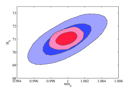
Figure 1: 2-D constraints on $\alpha$ and $H_{0}$ using Planck data (blue contours) and Planck+Euclid data (red contours).

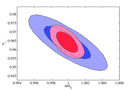
Figure 2: 2-D constraints on $\alpha$ and $n_{s}$ using Planck data (blue contours) and Planck+Euclid data (red contours).

In fact, as can be seen in Fig.3, using Euclid with Planck highlights a previously hidden degeneracy between $\alpha/\alpha_{0}$ and $\tau$; both these parameters do not affect the convergence power spectrum, thus they are not measured by Euclid, but they are both correlated with other parameters, such as $n_{s}$ (Fig.2 and Fig.4), whose constraints are improved through the analysis of weak lensing. This improvement on $n_{s}$ allows to clarify the degeneracy between $\alpha/\alpha_{0}$ and $\tau$. From this discussion is clear that a better determination of the optical depth $\tau$, through, for example, future measurements of the CMB polarization, would further improve the constraints on $\alpha$ and other parameters.

Clearly, as we can see from Table 3, when a variation of the fine structure constant is considered in the analysis, the gain of including Euclid is significantly reduced in the constraints of $n_{s}$ and $\tau$. As we can see also from Table 1, the errors on $n_{s}$ and $\tau$ are increased by $\sim 40\%$ and $\sim 57\%$ respectively when $\alpha$ is varying respect to the case when $\alpha$ is fixed to the standard value.

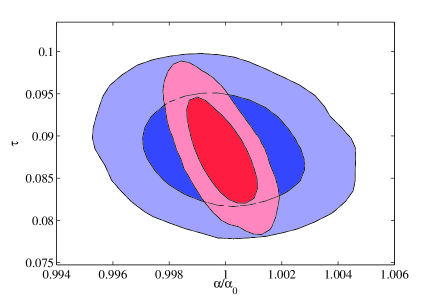
Figure 3: 2-D constraints on $\alpha$ and $\tau$ using Planck data (blue contours) and Planck+Euclid data (red contours).

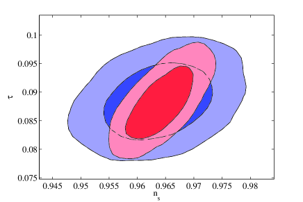
Figure 4: 2-D constraints on $n_{s}$ and $\tau$ using Planck data (blue contours) and Planck+Euclid data (red contours).

This however should not bring us to the decision of not varying $\alpha$ in the future analyses of those datasets. What indeed could happen if the true value of $\alpha$ is different from the standard one and we perform an analysis wrongly assuming $\alpha/\alpha_{0}=1$ ?

To answer to this question we have also analysed a mock dataset generated with $\alpha/\alpha_{0}=0.996$ (a variation in principle detectable with this future data) but (wrongly) assuming a standard value ($\alpha/\alpha_{0}=1$).

The results, reported in Tab.4, show a consistent and significant bias in the recovered best fit value of the cosmological parameters due to the strong degeneracies among $\alpha/\alpha_{0}$ and the Hubble constant $H_{0}$, the spectral index $n_{s}$ and the matter energy density $\Omega_{m}$ parameters.

	Planck+Euclid		Fiducial	$|\Delta/\sigma|$
			values
Model:	$\alpha/\alpha_{0}=1$	varying $\xi$
Parameter
$\Omega_{b}h^{2}$	$0.02232\pm 0.00010$	$0.02259\pm 0.00011$	$0.02258$	$2.7$
$\Omega_{c}h^{2}$	$0.1129\pm 0.00059$	$0.1106\pm 0.00078$	$0.1109$	$3.4$
$\tau$	$0.075\pm 0.0025$	$0.088\pm 0.0041$	$0.088$	$5.3$
$n_{s}$	$0.950\pm 0.0028$	$0.964\pm 0.0039$	$0.963$	$4.6$
$H_{0}$	$71.8\pm 0.30$	$71.0\pm 0.33$	$71.0$	$2.7$
$\Omega_{\Lambda}$	$0.737\pm 0.0032$	$0.736\pm 0.0034$	$0.735$	$0.6$
$\sigma_{8}$	$0.801\pm 0.0009$	$0.803\pm 0.0010$	$0.804$	$3.3$

Table 4: Best fit values and $68\%$ c.l. errors on cosmological parameters for the case in which a fiducial model with $\alpha/\alpha_{0}=0.996$ is fitted wrongly neglecting a variation in $\alpha$. The last column shows the absolute value of the difference between the best-fit value estimated fixing $\alpha/\alpha_{0}=1$ and the fiducial value, relative to the 1$\sigma$ error.

Note, from the results depicted in Figures 1, 2 and Figures 5 and 6 and also from the results in Tab. 4 that the shift in the best fit values is, as expected, orthogonal to the direction of the degeneracy of $\alpha/\alpha_{0}$ with these parameters. For example, lowering $\alpha$ damps the CMB small scale anisotropies. As we can from 1 this effect can be compensated by increasing $n_{s}$. Therefore a fiducial model with a lower value for $\alpha$ mimics a lower spectral index $n_{s}$, as shown in Tab. 4.

These results show that even for a small variation in $\alpha/\alpha_{0}\sim 0.5\%$, the best fit values recovered assuming that there is no variation in $\alpha$ can be at more than $95\%$ c.l. away from the correct fiducial values, and may induce a significant underestimation of $n_{s}$, $\tau$ and $\sigma_{8}$ and an overestimation of $H_{0}$. In the last column in Tab. 4 we show the difference between the wrong value estimated fixing $\alpha/\alpha_{0}=1$ and the fiducial value, relative to the 1$\sigma$ error. We note that also other parameters, as $\Omega_{c}h^{2}$ and $\Omega_{b}h^{2}$, have significant shifts.
When a variation of $\alpha$ is considered, the correct fiducial values are recovered, however at the expenses of less tight constraints.

Future analyses of high precision data from Euclid and Planck clearly need to consider possible deviations from the standard recombination scenario in order to avoid a significantly biased determination of the cosmological parameters.

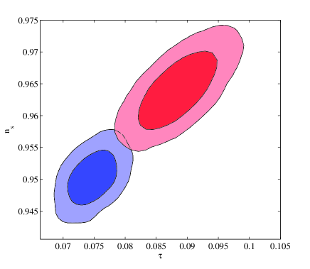
Figure 5: 2-D constraints on $n_{s}$ and $\tau$ using a fiducial model with $\alpha/\alpha_{0}=0.996$, fitting it with a fixed $\alpha/\alpha_{0}=1$ (blue contours) and with $\alpha/\alpha_{0}$ aloowed to vary (red contours).

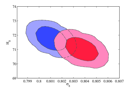
Figure 6: 2-D constraints on $\sigma_{8}$ and $H_{0}$ using a fiducial model with $\alpha/\alpha_{0}=0.996$, fitting it with a fixed $\alpha/\alpha_{0}=1$ (blue contours) and with $\alpha/\alpha_{0}$ aloowed to vary (red contours).

IV Conclusions

In this brief paper we have evaluated the ability of a combination of CMB and weak lensing measurements as those expected from the Planck and Euclid satellite experiments in constraining variations in the fine structure constant $\alpha$. We have found that combining the data from those two experiments would provide a constraint on $\alpha$ of the order of $\Delta\alpha/\alpha=8\times 10^{-4}$, significantly improving the constraints expected from Planck. These constraints can be reasonably futher improved by considering additional datasets. In particular, accurate measurements of large angle CMB polarization that could provide a better determination of the reionization optical depth will certainly make the constraints on $\alpha$ more stringent.

Moreover, we found that allowing in the analysis for variations in $\alpha$ has important impact in the determination of parameters as $n_{s}$, $H_{0}$ and $\tau$ from a Planck+Euclid analysis. We have shown that a variation of $\alpha$ of about $0.4\%$ can significantly alter the conclusions on these parameters.

Changing the fine structure constant by $0.4\%$ shifts the redshift at which the free electron fraction falls to $x_{e}=0.5$ by about $\sim 1\%$ from $z_{*}=1275$ to $z_{*}=1262$. An unknown physical process that delays recombination as, for example, dark matter annihilation (see e.g. silviab ), may have a similar impact in cosmological parameter estimation. Our conclusions can therefore be applied to the more general case of a modified recombination scenario.

V Acknowledgments

We are grateful to Tom Kitching, Luigi Guzzo, Henk Hoekstra e Will Percival for useful comments to the manuscript. We also thank Luca Amendola and Martin Kunz and the Euclid theory WG. This work is supported by PRIN-INAF, Astronomy probes fundamental physics. Support was given by the Italian Space Agency through the ASI contracts Euclid- IC (I/031/10/0).

References

- (1) E. Komatsu et al. [WMAP Collaboration], Astrophys. J. Suppl. 192, 18 (2011) [arXiv:1001.4538 [astro-ph.CO]] ; D. Larson et al., Astrophys. J. Suppl. 192, 16 (2011) [arXiv:1001.4635 [astro-ph.CO]].
- (2) B. A. Reid et al. [SDSS Collaboration], Mon. Not. Roy. Astron. Soc. 401, 2148 (2010) [arXiv:0907.1660 [astro-ph.CO]] ; B. A. Reid et al., Mon. Not. Roy. Astron. Soc. 404, 60 (2010) [arXiv:0907.1659 [astro-ph.CO]].
- (3) R. Amanullah et al., Astrophys. J. 716, 712 (2010) [arXiv:1004.1711 [astro-ph.CO]].
- (4) J. K. Webb, V. V. Flambaum, C. W. Churchill, M. J. Drinkwater and J. D. Barrow, Phys. Rev. Lett. 82, 884 (1999) [astro-ph/9803165]; J. K. Webb, M. T. Murphy, V. V. Flambaum, V. A. Dzuba, J. D. Barrow, C. W. Churchill, J. X. Prochaska and A. M. Wolfe, Phys. Rev. Lett. 87, 091301 (2001) [astro-ph/0012539].
- (5) J. K. Webb, J. A. King, M. T. Murphy, V. V. Flambaum, R. F. Carswell and M. B. Bainbridge, Phys. Rev. Lett. 107, 191101 (2011) [arXiv:1008.3907 [astro-ph.CO]].
- (6) J. -P. Uzan, Rev. Mod. Phys. 75, 403 (2003) [hep-ph/0205340].
- (7) P. P. Avelino et al., Phys. Rev. D 64 (2001) 103505 [arXiv:astro-ph/0102144]; C. J. A. Martins, A. Melchiorri, R. Trotta, R. Bean, G. Rocha, P. P. Avelino and P. T. P. Viana, Phys. Rev. D 66 (2002) 023505 [arXiv:astro-ph/0203149].
- (8) C. J. A. Martins, A. Melchiorri, G. Rocha, R. Trotta, P. P. Avelino and P. T. P. Viana, Phys. Lett. B 585, 29 (2004) [arXiv:astro-ph/0302295]; G. Rocha, R. Trotta, C. J. A. Martins, A. Melchiorri, P. P. Avelino, R. Bean and P. T. P. Viana, Mon. Not. Roy. Astron. Soc. 352, 20 (2004) [arXiv:astro-ph/0309211].
- (9) K. Ichikawa, T. Kanzaki and M. Kawasaki, Phys. Rev. D 74 (2006) 023515 [arXiv:astro-ph/0602577].
- (10) P. Stefanescu, New Astron. 12 (2007) 635 [arXiv:0707.0190 [astro-ph]].
- (11) M. Nakashima, R. Nagata and J. Yokoyama, Prog. Theor. Phys. 120 (2008) 1207 [arXiv:0810.1098 [astro-ph]].
- (12) E. Menegoni, S. Galli, J. G. Bartlett, C. J. A. Martins and A. Melchiorri, Phys. Rev. D 80 (2009) 087302 [arXiv:0909.3584 [astro-ph.CO]];
- (13) C. G. Scoccola, S. .J. Landau, H. Vucetich, Phys. Lett. B669 (2008) 212-216. [arXiv:0809.5028 [astro-ph]]; S. .J. Landau, C. G. Scoccola, [arXiv:1002.1603 [astro-ph.CO]].
- (14) E. Menegoni et al., International Journal of Modern Physics D, Volume 19, Issue 04, pp. 507-512 (2010).
- (15) E. Menegoni, M. Archidiacono, E. Calabrese, S. Galli, C. J. A. P. Martins and A. Melchiorri, arXiv:1202.1476 [astro-ph.CO].
- (16) [Planck Collaboration], arXiv:astro-ph/0604069.
- (17) R. Laureijs, J. Amiaux, S. Arduini, J. -L. Augueres, J. Brinchmann, R. Cole, M. Cropper and C. Dabin et al., arXiv:1110.3193 [astro-ph.CO]. Euclid Consortium website: http://www.euclid-ec.org
- (18) A. F. Heavens, 2003, MNRAS, 323, 1327
- (19) P. G. Castro, A. F. Heavens, T. D. Kitching, 2005, Phys. Rev. D, 72, 3516
- (20) A. F. Heavens, T. D. Kitching, A. N. Taylor, 2006, MNRAS, 373, 105
- (21) T. D. Kitching, A. F. Heavens, A. N. Taylor, M. L. Brown, K. Meisenheimer, C. Wolf, M. E. Gray, D. J. Bacon, 2007, MNRAS, 376, 771
- (22) S. Hannestad, H. Tu and Y. Y. Y. Wong, JCAP 0606 (2006) 025 [arXiv:astro-ph/0603019].
- (23) T. D. Kitching, A. F. Heavens, L. Verde, P. Serra and A. Melchiorri, Phys. Rev. D 77 (2008) 103008 [arXiv:0801.4565 [astro-ph]].
- (24) Bacon, D.; et al.; 2003; MNRAS, 363, 723-733
- (25) Massey R.; et al.; 2007, ApJS, 172, 239
- (26) Taylor, A. N.; et al.; 2004, MNRAS, 353, 1176
- (27) F. De Bernardis, M. Martinelli, A. Melchiorri, O. Mena and A. Cooray, Phys. Rev. D 84, 023504 (2011) [arXiv:1104.0652 [astro-ph.CO]]; M. Martinelli, E. Calabrese, F. De Bernardis, A. Melchiorri, L. Pagano and R. Scaramella, Phys. Rev. D 83 (2011) 023012 [arXiv:1010.5755 [astro-ph.CO]].
- (28) A. Lewis, A. Challinor and A. Lasenby, Astrophys. J. 538 (2000) 473.
- (29) T. Okamoto and W. Hu, Phys. Rev. D 67 (2003) 083002 [arXiv:astro-ph/0301031].
- (30) A. R. Cooray, Astron. Astrophys. 348 (1999) 31 [arXiv:astro-ph/9904246].
- (31) R. E. Smith et al. [The Virgo Consortium Collaboration], Mon. Not. Roy. Astron. Soc. 341 (2003) 1311 [arXiv:astro-ph/0207664].
- (32) L. Fu et al., Astron. Astrophys. 479 (2008) 9 [arXiv:0712.0884 [astro-ph]].
- (33) S. Galli, M. Martinelli, A. Melchiorri, L. Pagano, B. D. Sherwin and D. N. Spergel, Phys. Rev. D 82, 123504 (2010) [arXiv:1005.3808 [astro-ph.CO]].
- (34) S. Galli, F. Iocco, G. Bertone and A. Melchiorri, Phys. Rev. D 80 (2009) 023505 [arXiv:0905.0003 [astro-ph.CO]]; S. Galli, F. Iocco, G. Bertone and A. Melchiorri, Phys. Rev. D 84, 027302 (2011) [arXiv:1106.1528 [astro-ph.CO]].
- (35) A. Lewis and S. Bridle, Phys. Rev. D 66, 103511 (2002) (Available from http://cosmologist.info.)