Description and connection between the Oxygen order evolution and the superconducting transition in $La_{2}CuO_{4+y}$

Abstract

A recent hallmark set of experiments by Poccia et al in cuprate superconductors related in a direct way, for the first time, time ordering ($t$) of oxygen interstitials in initially disordered $La_{2}CuO_{4+y}$ with the superconducting transition temperature $T_{c}(t)$. We provide here a description of the time ordering forming pattern domains and show, through the local free energy, how it affects the superconducting interaction. Self-consistent calculations in this granular structure with Josephson coupling among the domains reveal that the superconducting interaction is scaled by the local free energy and capture the details of $T_{c}(t)$. The accurate reproduction of these apparently disconnected phenomena establishes routes to the important physical mechanisms involved in sample production and the origin of the superconductivity of cuprates.

1 Introduction

There are considerable evidences that the tendency toward phase separation is an universal feature of cuprate superconductors and others electronic oxides like manganites[1, 2]. The presence of hole-rich and hole poor phases were detected in oxygenated $La_{2}CuO_{4+y}$ almost immediately after the discovery of the superconductivity in these compounds[3] and in subsequent works[4, 5, 6, 7, 8]. Subsequent experiments have observed evidences of complexity and electronic disorder in many other materials[1, 2, 9].

In order to describe this phenomenon, some theories producing phase separation have been suggested, mainly based on doped Mott-Hubbard insulators. Some of these theories rely on Fermi-surface nesting, which leads to a reduced density of states or a gap at the Fermi energy[10, 11, 12, 13]. Others use a competition between the tendency of an antiferromagnetic insulator to expel doped holes and the long range Coulomb interaction to explain the formation of charge ordered phases[14, 15]. Another approach suggested that the pseudogap line $T^{*}$ is the onset of a first order transition, with the development of carriers of two types, frustrated by the electro-neutrality condition in the presence of rigidly embedded dopant ions[16, 17].

These theories describe some of the observed features, however they fail to predict some other basic experimental results, specially those related with real space inhomogeneities. Specifically, the recent combined experiment relating the time evolution ($t$) of the domain growth of oxygen interstitials (i-O) in $La_{2}CuO_{4+y}$ with the subsequent measurement of the superconducting transition temperature $T_{c}(t)$[18] brings new possibilities that require new approaches.

In this letter we propose a theory that provides an interpretation to the two parts of the Poccia et al experiment[18] and gives a clear explanation why the $T_{c}$ increases with the oxygen ordering. We rely on a description of the phase separation in cuprates based on the time-dependent Ginzburg-Landau or Cahn-Hilliard (CH) equation introduced earlier[20, 21]. We showed that the CH solutions yield granular regions where the free energy has two types of minima, for high and low doping, and that these valleys are surrounded by steep boundaries where the charges can get trapped, loosing part of their kinetic energy which enhances the mechanism of pair formation[22, 26]. During the phase separation process the free energy barrier between the two (high and low density) phases varies with the time which connects the time of oxygen ordering at high temperatures with the variations of the superconducting critical temperature $T_{c}(t)$ at low temperatures. Scaling the superconducting interaction with the local changes of the free energy is one of our most interesting finding. Another new point is that in this granular-like system the resistivity transition temperature $T_{c}$ occurs when the Josephson energy $E_{J}$ among the grains is equal to $K_{B}T_{c}$[26]. These new ideas are endorsed by the close agreement with the data as described below.

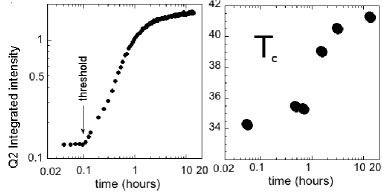
Figure 1: Graphs taken from Poccia et al[18]. On the left panel the presence of the reflected X-ray diffraction peaks associated with the oxygen order: we see that after a threshold, it increases rapidly and enter in a slow variation regime after a few hours. On the right panel, the corresponding measured values of $T_{c}(t)$ after the system being cooled down.

The connection between dopant atoms like the out of plane i-O[18, 23, 24] and the charges in the $CuO_{2}$ planes is well verified for $La_{2}CuO_{4+y}$, but it has also been seen in other cuprates[25]. It is an open question whether the electronic disorder is driven by the lower free energy of undoped antiferromagnetic (AF) regions[22] (intrinsic) or by the out of plane dopant’s (extrinsic origin)[25], like the i-O ordering[23, 18]. In either case, being intrinsic or extrinsic, it is very likely that there is an one to one correspondence between the two phenomena. This one to one correspondence is a crucial ingredient of our work and will be explored in detail here. Consequently the i-O ordering time evolution is assumed to occur together with the planar electronic phase separation (EPS) and they are described by the same CH equation[20, 21, 22, 26].

2 Phase Separation

Below the phase separation transition temperature $T_{ps}$, taken to be the order-disorder transition temperature for the i-O mobility at $T_{m}\approx 330$K[18], the appropriate order parameter is the normalized difference between the local $p(i,t)$ and the average charge density $p$ $u(p,i,t)\equiv(p(i,t)-p)/p$. Here, in order to compare with the actual system, we perform calculations with the optimal doping $p=0.16$, but we can perform calculations with any doping level. Clearly $u(i,t)=0$ corresponds to the homogeneous system, above $T_{PS}$, and $u(i,t)=\pm 1$ corresponds to the extreme case of full phase separation which is hardly achieved because the mobility vanishes as the temperature goes down. In this way one expects the system to reach an intermediated structure between homogeneous and complete phase separated. The Ginzburg-Landau (GL) free energy functional is the usual $u$ power expansion,

$$f(u)={{\frac{1}{2}\varepsilon^{2}|\nabla u|^{2}+V_{GL}(u,t)}}.$$ (1)

where the potential ${\it V_{GL}}(u,T)=-A^{2}(T)u^{2}/2+B^{2}u^{4}/4+...$, $A^{2}(T)=\alpha(T_{PS}(p)-T)$, $\alpha$ and $B$ are constants. $\varepsilon$ gives the size of the boundaries between the low and high density phases [20, 21]. The CH equation can be written[27] in the form of a continuity equation of the local density of free energy $f$, $\partial_{t}u=-{\bf\nabla.J}$, with the current ${\bf J}=M{\bf\nabla}(\delta f/\delta u)$, where $M$ is the mobility or the charge transport coefficient that sets the phase separation time scale. Therefore,

$$\frac{\partial u}{\partial t}=-M\nabla^{2}(\varepsilon^{2}\nabla^{2}u-A^{2}(T)u+B^{2}u^{3}).$$ (2)

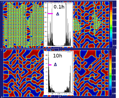
Figure 2: (color online) Time evolution simulation of the inhomogeneous charge density with average $p=0.16$ on an array of $105\times 105$ sites. The vertical scale gives the color code for the local densities (red is high and blue is low density). Top panels are for $t=2000ts$ end $t=4000ts$. Lower panels are for the $t=20.000$ and $t=200.000ts$. In top middle the local density $p(i)$ histogram for the $t=2000ts\equiv 0.1h$. In the lower panel the histogram for $t=200.000ts\equiv 10h$. The estimated FWHM of the charge dispersion $\Delta$ marked in the plots are to be compared with the experimental values.

The phase separation process described by this CH differential equation occurs due to the minimization of the free energy given by Eq.(1). The parameter $\varepsilon$ determines the size of the grain boundaries and $A(T)/B$ the values of the order parameter at the minima near the transition temperature. If $A(T)$ is zero (above $T_{ps}$) there is only one solution for the free energy and for the non-vanishing case there are two solution corresponding to the two phases (high and low densities)[27]. In Fig.(2), we show some typical simulations of the density map with the two (hole-rich and hole-poor) phases given by different colors. The simulations were done with $\varepsilon=0.08$ and $A(T)/B=1$. We use a constant value for the $A(T)/B$ ratio because usually the phase separation occurs in a small temperature interval and the mobility ceases at low temperatures.

In the case of the i-O experiments[18] the system is heated to $T=370$K above the mobility temperature $T_{m}=330$K and quenched to low temperature. Such procedure does not yield ordered i-O peaks and has poor superconducting order. However, by irradiating a given compound with X-rays near T=300K, Poccia et al[18] observed, after a time threshold $t_{0}$, the evolution of nucleation and growth of ordered domains accompanied by the recovery of a robust high $T_{c}$ state.

Here, we simulate the nucleation of these ordered domains following the EPS time evolution. In the simulations on a $105\times 105$ lattice, we note that below t=250ts (ts$\equiv$time steps) the system has an uniform density but at t=265ts a non uniformity with a regular checkerboard pattern sets in. The high and low densities increase up to 2000ts when another domain pattern, more irregular, develops as it is shown in Fig.2a. At 4000ts, the checkerboard order rests only on less than 1/3 of the system and the more stable irregular granular order dominates, as shown in Fig.2b. We make a correspondence between these ordered and disordered structure and that described by Fratini et al[23], i.e., a system with two phases and two different $T_{c}$s. Above 6000ts the granular pattern dominates and from 20000ts (Fig.2c) to 200000ts (Fig.2d) the grains grow very slowly. To make a direct comparison with the experiments, we take the onset or threshold time of the stable phase, i.e., $t_{0}=2000$ts or 0.1h as the beginning of the i-O process. This connects in a simple way the oxygen ordering at larger irradiated times with the raise and grow of the stable domains shown in Fig.(2).

In the CH approach, another way to follow a phase separation process is through the local densities histograms. In Fig.(2) we show this possibility for two selected times and as expected, the histogram dispersion $\Delta(t)$ decreases as time increases. We compare directly the two dispersions, the calculated from histograms, like those displayed in Fig.(2), and the experimental data in Fig.(3), without any adjustable parameter.

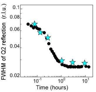
Figure 3: (color online) The FWHM of the i-O X-rays diffracted dispersion peaks [18] and the values of the local densities histograms $\Delta(t)$ calculated from 6 different times density maps dispersion (blue stars) as shown in Fig.(2 .

3 The local free energy and the pair formation

The CH equation yields the phase separation order parameter $u(i,T)$, that is used to calculate the potential $V_{GL}(i,t)$ from free energy (Eq.(1)). This is shown by the 3D view map in Fig.(4) for the case of t=10h. It is also shown in the left panel the values of $V_{GL}(i,t)$ along 25 sites in a straight line in the middle of the view map of Fig.(4) for four different times of phase separation or X-ray irradiation. In this way, we can visualize the regions where the charges get trapped. The inset shows the time variations of the barrier walls that, by assumption, scale the superconducting interaction[28].

The calculations shown in the inset of Fig.(4) demonstrate how it is possible to connect the phase separation time with the height of the $V_{GL}(i,t)$ grain boundary walls, which we define as $V_{gb}(t)$. The effect of $V_{gb}$ on the charges is to trap them inside the grains, and consequently they lose part of their kinetic energies. This loss of kinetic energy in the presence of a two-body attractive potential favor the possibility of Cooper pair formation and the domain walls act as a catalyst to the superconducting state[28]. The small changes on the size of $V_{gb}(t)$ with the time of phase separation $t$, as shown if Fig.(4), affects strongly the superconducting properties. The figure shows the larger increase between $t=0.3h=6000ts$ and $5h=100000ts$, right before it saturates.

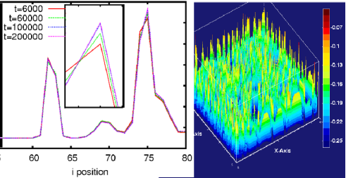
Figure 4: (color online) A 3D view map of the potential ${\it V_{GL}}(i,t=10h)$ on the right panel. On the left, the values on 25 sites in row to visualize the structure of the free energy potential wells with walls that leads to the definition of $V_{gb}(t)$ in the text. The values of $V_{gb}(t)$ are shown here at $t=0.3h,3h,5h$ and $10h$ and are very similar. In the inset we blow up the peaks and we see clearly a steady increase between $t=0.3h=6000ts$ and $t=5h=100000ts$ and the saturation above $t=5h$. The relative variations on $V_{gb}(t)$ are very small but have an important role in the BdG calculations of $\Delta_{d}(t)$ and on the $T_{c}(t)$.

4 The Superconducting Calculations

The calculated density maps $p(i,t)$ on a square lattice like that of Fig.(2) are used as the initial input and it is alway maintained fixed through the self-consistent Bogoliubov-deGennes (BdG) calculations. This is because it represents the situation in which the system is quenched to low temperatures to measured $T_{c}$. We use nearest neighbor hopping $t_{ij}=0.15$eV and next nearest neighbor hopping $t_{1}/t_{ij}=-0.27$ taken from hole doped experimental dispersion relations[29]. For completeness, the BdG equations are[22, 21, 30].

$$\begin{pmatrix}K&\Delta\cr\cr\Delta^{*}&-K^{*}\end{pmatrix}\begin{pmatrix}u_{n}({\bf x_{i}})\cr\cr v_{n}({\bf x_{i}})\end{pmatrix}=E_{n}\begin{pmatrix}u_{n}({\bf x_{i}})\cr\cr v_{n}({\bf x_{i}}).\end{pmatrix}$$ (3)

These equations, defined in detail in Refs.[21, 30], are solved self-consistently. $u_{n}$, $v_{n}$ and $E_{n}\geq 0$ are respectively the eigenvectors and eigenvalues. The d-wave pairing amplitudes are given by

$$\Delta_{d}({\bf x}_{i}) = -{V_{gb}\over 2}\sum_{n}[u_{n}({\bf x}_{i})v_{n}^{*}({\bf x}_{i}+{\bf\delta})+v_{n}^{*}({\bf x}_{i})u_{n}({\bf x}_{i}$$ (4)

$$+{\bf\delta})]\tanh{E_{n}\over 2k_{B}T},$$

and the local inhomogeneous hole density is given by

$$p({\bf x}_{i})=1-2\sum_{n}[|u_{n}({\bf x}_{i})|^{2}f_{n}+|v_{n}({\bf x}_{i})|^{2}(1-f_{n})],$$ (5)

where $f_{n}$ is the Fermi function. We stop the self-consistent calculations only when all $p({\bf x}_{i})\equiv p(i)$ converges to the appropriate time CH density map like those shown in Fig.(2) or in Fig.(5).

Typical solutions can be visualized in Fig.(5) where we show the local density $p(i)$ on a square lattice of 28x28 sites where the BdG calculations were made and the 3D map of the low temperature amplitude of the $d_{x^{2}-y^{2}}$ order parameter $\Delta_{d}(i,T\approx 0K)[cos(k_{x})-cos(k_{y})]$. The pairing potential $V_{gb}(t)$ in unities of $eV$ is parametrized to yield the average local density of states (LDOS) gaps measured by low temperature STM on the optimal doping $p=0.16$ $La_{2-p}Sr_{p}CuO_{2}$ [31], namely, $\Delta_{d}(T\approx 0)\approx 7-12$meV. Starting with $V_{gb}(t=2000ts)=0.95t$, and analyzing the increase of $V_{gb}(t)$ as those shown in Fig.(4), we were able to connect the time of X-ray exposure to the superconducting amplitudes.

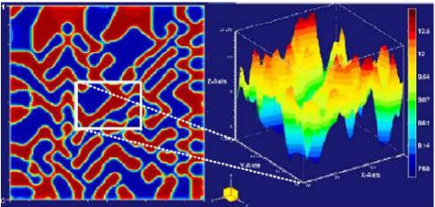
Figure 5: (color online) Left panel shows a typical density view map and the 28x28 square where the local superconducting amplitudes $\Delta_{d}(i,t)$ are calculated by the BdG approach at $t=6000ts\equiv 0.3$h, as an example.

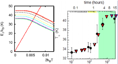
Figure 6: (color online) Left panel, the thermal energy $k_{B}T$ and the Josephson coupling among superconducting grains $E_{J}(t,T)$ (as given by Eq.(6)) for some given time of irradiation $t$ as function of T. The intersections give the calculated results for $T_{c}(t)$ plotted with inverted triangles on the top of the experimental results in the right panel.

With these values of the potential and the corresponding $\Delta_{d}(i,T\approx 0)$, we find that $\Delta_{d}(i,T)\rightarrow 0$ at a single temperature $T^{*}\approx 96$K, which is much larger than typical values of $T_{c}(p=0.16)$ for $La_{2}CuO_{4+y}$, but in agreement with the pseudogap phase measured by STM[32], or the Nernst signal on LSCO[33, 34]. To obtain the measured values of $T_{c}$, we notice that the EPS transition, with the free energy walls and wells, makes the structure of the system similar to granular superconductors[35]. In this way, it is likely that the superconducting transition occurs in two steps[26, 28]: first by intra-grain superconductivity and than by Josephson coupling with phase locking at a lower temperature. This two steps approach is also supported by the two energy scales found in most cuprates[36, 37], and also in the two different regimes of critical fluctuations in $YBa_{2}Cu_{3}O_{7}$ single crystals[38].

Granular superconductors are often modeled as networks of Josephson junctions (weak links) connecting the grains, i.e., the Josephson network[39]. In the case of an order parameter with $d_{x^{2}-y^{2}}$ symmetry, the direction of the tunnel matrix element across a junction is essential and it was analyzed in detail[40, 41, 42]. In the special relative orientation for which the d-wave gap nodes in both side of the junction are parallel, the critical current behaves mostly like an s-wave superconductor and its temperature dependence is qualitatively the same (see, for instance, Fig.3a of Bruder et al[42]). In the EPS considered here with the electronic grains in a $La_{2}CuO_{4+y}$ single crystal, the superconducting order parameter in each grain has the same orientation in real space, with the nodes along the crystal axis. Then the Josephson coupling is determined by tunneling from a gap node in one grain into the corresponding node of another grain[40, 41, 42].

Based on this similar behavior and on this special orientation, we use the analytical expression of the Josephson coupling energy $E_{J}$ to two s-wave superconductors[43]

$$E_{J}(t,T)\approx\frac{\pi h\Delta^{av}_{d}(t,T)}{4e^{2}R_{n}}tanh(\frac{\Delta^{av}_{d}(t,T)}{2K_{B}T}),$$ (6)

as an approximation to obtain the relative changes of $E_{J}$ with the irradiation time.

In this way the increase of the potential by the phase separation process enters in this equation by the values of $\Delta^{av}_{d}(T,t)$. Here $\Delta^{av}_{d}(T,t)\equiv\sum_{i}^{N}\Delta_{d}(T,i,t)/N$, since the amplitude $\Delta_{d}(T,i,t)$ varies with the position $i$ within the crystal, as shown in the right panel of Fig.(5). $R_{n}$ is the normal resistance of the $La_{2}CuO_{4+y}$ compound, which we assume to be independent of the time as inferred from the data of Poccia et al[18]. It is also proportional to the planar resistivity $\rho_{ab}$ measurements[44] on the $La_{2-p}Sr_{p}CuO_{2}$ series. In Fig.(6), the Josephson coupling $E_{J}(p,T)$ is plotted together with the thermal energy $K_{B}T$. The intersections yield $T_{c}(t)$.

As discussed in connection with the free energy of Eq.(1) and Fig.(4), the relative values of the grain boundary potential wall $V_{gb}(t)$ are easy to estimate, but we do not know their absolute values. As already mentioned, we use $V_{gb}(t=0.2h)=0.95t\approx 0.14$eV that matches the 1st point of Poccia et al[18], namely, $T_{c}(t=0.2h)=33.6$K. All the others $T_{c}(t)$ results for larger $t$, shown in Fig.(6), follow by the small but steady variations in $V_{gb}(t)$ shown in the inset of Fig.(4). In other words, we use $V_{gb}(t=0.2h)$ as an adjustable parameter to obtain $T_{c}(t=0.2h)$, but all the others seven points shown in the right panel of Fig.(6) are parameter free, i.e., they follow from the increase of $V_{gb}(t)$ as shown in Fig.(4). The steep increase of $T_{c}(t)$ during the consolidation of the stable phase between $t\approx 0.3-5h$ agrees well with the data as shown in Fig.(6), indicating that our triple approach (CH simulation of $p(i)$, the local $\Delta_{d}(i,t)$ and the Josephson estimation of $T_{c}(t)$ is appropriate to describe the $La_{2}CuO_{4+y}$ properties.

5 Conclusions

We have provided a complete description of a novel set of complex experiments relating the time of sample preparation with the superconducting temperature $T_{c}(t)$. The ensemble of calculations reported here demonstrated that the local variations in the free energy developed during the phase separation process is an essential ingredient of the superconducting interaction. These findings reveal a virtually unexplored line of research on how systematic variations of sample preparation may affect the superconductors properties.

I gratefully acknowledge partial financial aid from Brazilian agencies FAPERJ and CNPq.

References

- [1] \NameEd.by Sigmund E. Muller K.A. \BookPhase Separation in Cuprate Superconductors \PublSpringer-Verlag, Berlin \Year1994.
- [2] \NameDagotto E. \BookNanoscale Phase Separation and Colossal Magneto-Resistance \PublSpringer, Berlin \Year2002.
- [3] \NameJorgensen J.D. et al \REVIEWPhys. Rev. B38 198811337.
- [4] \Name Grenier J.C. at al \REVIEW Phys. C2021992209.
- [5] \Name Radaelli P.G. et al \REVIEWPhys. Rev. B48 1993499.
- [6] \Name Wells B.O. et al \REVIEWScience27719971067.
- [7] \NameCampi G. \REVIEWJ. Supercond. Nov. Magn.172004137.
- [8] \NameLee Y.S. \REVIEWPhys. Rev. B69 2004020502.
- [9] \NameBianconi A. Saini N.L. \BookStripes and related phenomena, Selected topics in Superconductivity \PublKluwer Academic/Plenum Publishers \Year2000. \revision
- [10] \NamePoilblanc D. Rice T.M. \REVIEWPhys. Rev. B39 19899749.
- [11] \NameMachida K. \REVIEWPhysica C158 1989192.
- [12] \NameZaanen J. Gunnarsson O. \REVIEWPhys. Rev. B40 19897391.
- [13] \NameSchulz H. \REVIEWPhys. Rev. Lett.64 19901445.
- [14] \Name Emery V.J. Kivelson S.A. \REVIEWPhysica C209 1993597.
- [15] \Name Löw U. et al \REVIEWPhys. Rev. Lett. 72 19941918.
- [16] \NameGorkov L.P. Teitel’baum G.B. \REVIEWPhys. Rev. Lett. 97 2006 247003.
- [17] \NameGorkov L.P Teitel’baum G.B. \REVIEWPhys. Rev.B 77 2008 180511.
- [18] \NamePoccia N. et al \REVIEWNature Materials 10 2011733.
- [19] \NameCahn J.W. Hilliard J.E. \REVIEWJ. Chem. Phys 281958 258.
- [20] \NameDe Mello E.V.L. Silveira Filho Otton T. \REVIEWPhysica A3472005 429.
- [21] \Name De Mello E.V.L. Caixeiro E.S. \REVIEW Phys. Rev. B702004224517.
- [22] \NameDe Mello E.V.L, Passos C.A.C Kasal R.B. \REVIEWJ. Phys.: Condens. Matter 21 2009 235701.
- [23] \NameFratini Michela et al \REVIEWNature 466 2010 841.
- [24] \NameRicci A. et al \REVIEWPhysical Review B84 2011 060511.
- [25] \NameOfer Rinat, Keren Amit \REVIEWPhys. Rev. B80 2009 224521.
- [26] \NameDe Mello E.V.L. Kasal R.B. \REVIEWJ. Supercond. Nov. Magn. 242011 1123.
- [27] \NameBray A.J. \REVIEWAdv. Phys. 431994347.
- [28] \NameDe Mello E.V.L. Kasal R.B. \REVIEW Phys. C 472201260.
- [29] Schabel M.C., Park C.-H., Matsuura A., Shen Z.X., Phys. Rev. B 57, 6090 (1998).
- [30] \NameDias D.N. et al \REVIEWPhys. C4682008480.
- [31] \NameKato T. et al \REVIEW J. Phys. Soc. Jpn. 772008054710.
- [32] \Name Gomes Kenjiro K. et al \REVIEWNature 447 2007 569.
- [33] \NameWang Yayu , Li Lu Ong N.P. \REVIEWPhys. Rev. B 73 2006 024510.
- [34] \NameDe Mello E.V.L. Dias D.N. \REVIEWJ. Phys.C.M. 192007 086218.
- [35] \NameMerchant L. et al \REVIEWPhys. Rev. B63 2001 134508.
- [36] \NameDamascelli A., Shen Z.X. Hussain Z., \REVIEW Rev. Mod. Phys. 752003473.
- [37] \NameGuyard W. et al \REVIEWPhys. Rev. Lett. 1012008097003.
- [38] \Name Costa Rosangela M. et al \REVIEWPhys. Rev. B642001 214513.
- [39] \NameEbner C. Stroud D. \REVIEWPhys. Rev. B311985 165.
- [40] \NameSigrist Manfred Rice T.M. \REVIEWRev. Mod. Phys. 67 1995 503.
- [41] \NameBarash Yu.S. et al \REVIEWPhys. Rev. B521995665.
- [42] \NameBruder C. et al \REVIEWPhys. Rev. B51 1995R12904.
- [43] \NameAmbeogakar V. Baratoff A. \REVIEW Phys. Rev. Lett. 101963486.
- [44] \NameTakagi H. et al \REVIEWPhys. Rev. Lett. 69 19922975.