OVERVIEW: This report presents a unified treatment of the density of states for the knots and folds of polymer chains. The physical realization of such systems ranges from DNA molecules (Taylor) to the microscopic configurations of space-time (Rovelli,Baez). Explicit calculations employing this procedure will appear in a subsequent paper.

The method in brief is as follows:
1. the starting point is a straight line/chain connecting two boundaries A and B as shown in Fig 1
2. the line is bent at each node, starting at one end and successively moving down the length of the chain one node at a time
3. at each point where the chain crosses itself a ”cross-over/under” is assigned
4. a complete set of configurations, the function space of the knot/fold, is obtained by allowing all possible folds/crossings (sequences of folds/crossings are characterized by binary strings)
5. a matrix construction is used to characterize the topologically distinct configurations; we comment on the implied curvature of the resulting space


bobk@physics.wisc.edu

PART A: folds

Motivation

It has been said that the phenomenon of polymer folding is an intractable physics problem, yet at first glance the problem appears to be well suited to the machinery of statistical mechanics: first choose a model pair potential between joints in the chain, then use the total energy in the Boltzmann factor and sum over all possible configurations. Iteration of this procedure then follows by suitable adjustments to the assumed pair potential. A difficulty arises in that the pair potential is likely to be dependent on the entire configuration; this is almost certainly due to quantum mechanical influence on the electron orbitals that determine the pair potential. Failure of statistical mechanical models suggests the need to separate energy and configurational considerations.

1. Statistical Mechanics

Models of the self-avoiding walk are frequently used to describe the quantitative properties of polymer/protein chain folding (Freed, Pande et al, Amit et al). Typically these tools employ standard methods in statistical mechanics. A multi-particle Hamiltonian is set up

$$H=\sum_{i,j}V(x_{i},x_{j})$$

representing a fictitious energy of interaction between two elements in the chain located at $x_{i}$ and $x_{j}$ . The statistical properties of the chain are then obtained from analysis of the partition function

$$Z=\int D[x_{i}]e^{-\beta H}$$

where $\beta$ acts as an inverse temperature parameter. It is a straight forword procedure to evaluate this quantity, but because the interactions must be strong to effectively eliminate configurations where the chain crosses itself, standard perturbative techniques are of limited value.

Evaluation of the partition function is not trivial of course, but nevertheless provides a complete and systematic solution to the problem. The objection to this approach is that the effective/model potential is likely to be unrepresentative. The energy of interaction between sites is unavoidably quantum mechanical and thus the interaction will vary not just on distance between pairs but also on total chain configuration (Bryngelson 1994). Typically, simulations have found the need for what are called non-native interactions (Wallin et al) in order to match with experiment.

To this extent we set energy considerations aside and limit the discussion to configurational concerns. Exact pair interaction must almost always depend on total configuration, hence, non-native interactions.

2. The Folding Operator

Each initial chain is a line on the interval $[0,N]$. Each fold describes a bend of $\pm\frac{\pi}{2}$, the first bend being at the node $N-1$, the second at $N-2$, etc. A binary string $[00101...011]$ is used to charcterize the $\pm$ sequence for one complete fold, while a second is used to describe the set of crossings as shown in Fig 1. The matrices that perform this operations are as follows.

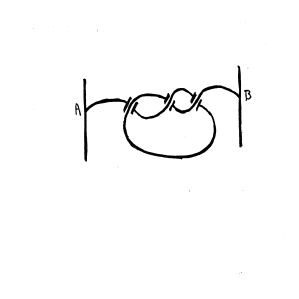
Figure 1: typical configuration, in this case $3_{1}$, the trefoil

Figure 2: typical bent polymer without crossings

The definition of the folding operator is that it bends, at right angles, an initially straight chain, one site after another. There is one such operator, or matrix in this formulation, for each configuration, ignoring self-intersections, and it will be the goal of the analysis to pick out those matrices that create allowable configurations.

The folding operator is easy to construct and relatively easy to diagonalize but we will find limits to the extent of useful information obtained.

In general the rotation operator takes the form

$$\tau(\theta)=\left[\begin{array}[]{cc}\cos(\theta)&\sin(\theta)\\ -\sin(\theta)&\cos(\theta)\\ \end{array}\right]$$

where $\theta$ is the clockwise angle of rotation from the positive x-axis (3 o’clock position). For $\theta=\frac{\pi}{2}$

$$\tau(\frac{\pi}{2})=\left[\begin{array}[]{cc}0&1\\ -1&0\\ \end{array}\right]\equiv\tau$$

Define $I_{n}=diag(1,1,...,1)$ n elements. For a chain of n+1 sites set from (0,0) to (n,0), folding at the second to the last site is

$$I_{n-2}\oplus\left[\begin{array}[]{c c }1&\\ \sigma_{1}&\tau_{1}\\ \end{array}\right]$$

where $\tau_{l}=s_{l}\tau$, $s=\pm 1$; folding at site third from the end is

$$I_{n-3}\oplus\left[\begin{array}[]{c c c}1&&\\ \sigma_{2}&\tau_{2}&\\ \sigma_{2}&&\tau_{2}\\ \end{array}\right]$$

etc.

For example, successive applications of the first four of these matrices yields

$$\left[\begin{array}[]{ccccc}1&&&&\\ \sigma_{4}&\tau_{4}&&&\\ \sigma_{4}&\tau_{4}\sigma_{3}&\tau_{43}&&\\ \sigma_{4}&\tau_{4}\sigma_{3}&\tau_{43}\sigma_{2}&\tau_{432}&\\ \sigma_{4}&\tau_{4}\sigma_{3}&\tau_{43}\sigma_{2}&\tau_{432}\sigma_{1}&\tau_{4-1}\\ \end{array}\right]$$

where $\sigma_{n}=1-\tau_{n}$, and $\tau_{432}=s_{4}s_{3}s_{2}\tau^{3}$.

These are random matrices to be dealt with in the follow-up paper where we discuss the distribution of eigenvalues. Preliminary numerical studies suggest allowed structures tend to cluster in groups. Such behavior has been reported in previous studies (Balafras and Dewey, Moret et al) and has possible application to the so-called Levinthal Paradox (Karplus, Dill and Chan).

The Levinthal Paradox says that a large polymer would take eons rather than milliseconds to fold if it did so by randomly sampling accessible states. What this suggests is that the folding process (and knotting as well) is accomplished through some globally determined energy potential and is not a locally driven phenomenon (Wallin et al).

Part B: Knots

Motivation

The difference between a knot and a fold in this formulation of the problem is the nature of the sequence of crossings: a particular sequence of crossings may, or may not, actually tie the chain, such that it becomes possible, or not, to pull the two ends arbitrarily far apart, returning the chain to the initial straight line.

How to do this is dealt in part by the following scheme. Each knot is thought to be described by two dimensions, position (or crossing) and time (or path length). The distinction as suggested in Fig 3 is made by first labeling all crossings successively until each site has a number, followed by assigning to each site a ”time” value as a full circuit of the knot is traversed.

[Aside: For the first few knots all crossings are labeled before the return path is begun; these are called sequential. However, beginning with $7_{7}$ a previously labeled site is encountered before all seven sites have been labeled; these are called nonsequential. This is something like Euler’s Konigsberg Bridge problem. This distinction is made clear in Figs 4 and 5 where we show how to reduce $6_{3}$ to a simpler circuit, thus making it clear that the knot is sequential, and also show that $7_{7}$ is necessarily nonsequential.]

1. Knot Matrix Designation

For a knot with N crossings:

a) each crossing is an element in a sequence of positions
b) the $n^{th}$ position element is described by the matrix

$$T_{n}(t)=\left[\begin{array}[]{ccc}I_{n-1}&&\\ &\tau(t)&\\ &&I_{N-n-1}\\ \end{array}\right]$$

where

$$\tau(t)=\left[\begin{array}[]{ccc}0&e^{i\alpha t}\\ 1&0\\ \end{array}\right]$$

for cross-over and $\tau^{\dagger}$ for cross-under; $\alpha$ to be determined.
c) the time sequence for a given knot is the product $[T]=T_{a}T_{b}T_{c}T_{d}...$ where $abcd...$ are successive crossings visited on a complete path; for example for $6_{1}$ the $[T]$ product is $\bar{T}_{5}T_{6}\bar{T}_{1}T_{2}\bar{T}_{3}T_{4}\bar{T}_{6}T_{5}\bar{T}_{4}T_{3}\bar{T}_{2}T_{1}$ abbreviated to $[\bar{5}6\bar{1}2\bar{3}4.\bar{6}5\bar{4}3\bar{2}1]$. This procedure is not unlike the group theory method of Artin/Burau (Kauffman, p. 86) except that the operators are 2d and label crossings instead of braids (Birman and Brendle). Also it appears that these matrices do not obey the Yang-Baxter relations (Baez and Muniain).
d) as in Fig 3 each operator is 2d, i.e. $T_{a}(n)$ where (a,n)=(space,time)=(position,path length).

The matrices $\tau,\tau^{\dagger}$ act at each crossing something like raising and lowering operators in field theory, and create a ”time evolution” of the initial, ground state (the identity matrix), carrying it through a sequence of intermediate states. The resulting matrix is a measure of the curvature of the knot to the extent that the configuration is not returned to the identity matrix for the closed contour.

Figure 3: geometry of the matrix $T_{l}(n)$

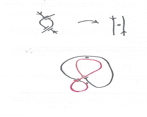
Figure 4: construction showing that $6_{3}$ is sequential

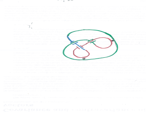
Figure 5: construction showing that $7_{7}$ is not sequential

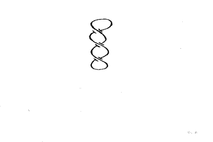
Figure 6: the identity operation for N=3

2. Topological Subspaces; Curvature

In order to construct the representative matrices for each knot we need to assign a value to the time variable $e^{i\alpha}$ and this is accomplished by requiring that configurations isomorphic to the unknot give the identity as shown in Fig 6. For numerical purposes we can choose an arbitrary real number $q$ and require that the second pass through the crossings act in reverse time; for example for $4_{1}$ the time factors are $q,q^{2},q^{3},q^{4},q^{4},q^{3},q^{2},q$.

The resulting matrices act as a representation of the curvature of the knot in the sense that a complete path around the knot is analogous to the closed curve in the computation of parallel displacement of a vector defined on a smooth manifold. The resulting matrix bares some relation to the curvature tensor in differential geometry; in quantum field theory, this quantity is a relation of the Wilson Loop, without the extra machinery for field theory purposes.

The table below gives the knot, the path and the resulting matrices for the figures shown in the Appendix.

[Aside: I gave up trying to get LATEX to put the figures where I wanted. The Appendix included here contains the relevant knots of the table; the drawings, inexpert as they are, indicate the sequence of crossings used to obtain the matrices below.]

$$\begin{array}[]{c c c}3_{1}&[\bar{3}2\bar{1}.3\bar{2}1]&\left[\begin{array}[]{cc|cc}&&1&\\ &&&q^{-5}\\ \hline\cr q^{2}&&&\\ &q^{3}&&\\ \end{array}\right]\\ \hline\cr 4_{1}&[\bar{3}4\bar{1}2.\bar{4}3\bar{2}1]&\left[\begin{array}[]{ccc|cc}&&&q^{-7}&\\ &q^{2}&&&\\ q^{4}&&&&\\ \hline\cr&&1&&\\ &&&&1\\ \end{array}\right]\\ \hline\cr 5_{1}&[\bar{5}4\bar{3}2\bar{1}.5\bar{4}3\bar{2}1]&\left[\begin{array}[]{ccc|ccc}&&1&&&\\ &&&q^{-7}&&\\ &&&&1&\\ \hline\cr&&&&&q^{-7}\\ q^{6}&&&&&\\ &q^{5}&&&&\\ \end{array}\right]\\ \hline\cr 5_{2}&[\bar{5}4\bar{1}2\bar{3}.5\bar{4}3\bar{2}1]&\left[\begin{array}[]{ccc|ccc}&&&&q^{-4}&\\ &q^{2}&&&&\\ &&1&&&\\ \hline\cr&&&&&q^{-7}\\ q^{6}&&&&&\\ &&&q^{3}&&\\ \end{array}\right]\\ \hline\cr\end{array}$$

$$\begin{array}[]{c c c}6_{1}&[\bar{5}6\bar{1}2\bar{3}4.\bar{6}5\bar{4}3\bar{2}1]&\left[\begin{array}[]{cccc|ccc}&&&&&q^{-15}&\\ &q^{2}&&&&&\\ &&1&&&&\\ &&&q^{2}&&&\\ \hline\cr q^{10}&&&&&&\\ &&&&1&&\\ &&&&&&1\\ \end{array}\right]\\ \hline\cr 6_{2}&[\bar{5}4\bar{3}6\bar{1}2.\bar{6}5\bar{4}3\bar{2}1]&\left[\begin{array}[]{cccc|ccc}&&&q^{-9}&&&\\ &q^{4}&&&&&\\ &&&&1&&\\ &&&&&q^{-7}&\\ \hline\cr q^{8}&&&&&&\\ &&q^{4}&&&&\\ &&&&&&1\\ \end{array}\right]\\ \hline\cr 6_{3}&[\bar{3}6\bar{5}2\bar{1}4.\bar{6}5\bar{4}3\bar{2}1]&\left[\begin{array}[]{cccc|ccc}&&1&&&&\\ &&&q^{-7}&&&\\ &&&&&q^{-11}&\\ &&&&&&1\\ \hline\cr&q^{5}&&&&&\\ q^{10}&&&&&&\\ &&&&q^{3}&&\\ \end{array}\right]\\ \hline\cr 7_{1}&[\bar{7}6\bar{5}4\bar{3}2\bar{1}.7\bar{6}5\bar{4}3\bar{2}1]&\left[\begin{array}[]{cccc|cccc}&&1&&&&&\\ &&&q^{-9}&&&&\\ &&&&1&&&\\ &&&&&q^{-9}&&\\ \hline\cr&&&&&&1&\\ &&&&&&&q^{-9}\\ q^{12}&&&&&&&\\ &q^{15}&&&&&&\\ \end{array}\right]\\ \hline\cr\end{array}$$

$$\begin{array}[]{c c c}7_{2}&[\bar{7}6\bar{1}2\bar{3}4\bar{5}.7\bar{6}5\bar{4}3\bar{2}1]&\left[\begin{array}[]{cccc|cccc}&&&&&&q^{-10}&\\ &q^{2}&&&&&&\\ &&1&&&&&\\ &&&q^{2}&&&&\\ \hline\cr&&&&1&&&\\ &&&&&&&q^{-9}\\ q^{12}&&&&&&&\\ &&&&&q^{3}&&\\ \end{array}\right]\\ \hline\cr 7_{3}&[\bar{5}6\bar{7}4\bar{3}2\bar{1}.7\bar{6}5\bar{4}3\bar{2}1]&\left[\begin{array}[]{cccc|cccc}&&1&&&&&\\ &&&q^{-9}&&&&\\ &&&&1&&&\\ &&&&&q^{-9}&&\\ \hline\cr q^{10}&&&&&&&\\ &q^{12}&&&&&&\\ &&&&&&1&\\ &&&&&&&q^{-4}\\ \end{array}\right]\\ \hline\cr 7_{4}&[\bar{5}6\bar{7}4\bar{1}2\bar{3}.7\bar{6}5\bar{4}3\bar{2}1]&\left[\begin{array}[]{cccc|cccc}&&&&q^{-6}&&&\\ &q^{4}&&&&&&\\ &&1&&&&&\\ &&&&&q^{-9}&&\\ \hline\cr q^{10}&&&&&&&\\ &&&q^{5}&&&&\\ &&&&&&1&\\ &&&&&&&-q^{4}\\ \end{array}\right]\\ \end{array}$$

$$\begin{array}[]{c c c}7_{5}&[\bar{7}6\bar{3}2\bar{1}4\bar{5}.7\bar{6}5\bar{4}3\bar{2}1]&\left[\begin{array}[]{cccc|cccc}&&1&&&&&\\ &&&q^{-7}&&&&\\ &&&&&&q^{-6}&\\ &q^{7}&&&&&&\\ \hline\cr&&&&1&&&\\ &&&&&&&q^{-9}\\ q^{12}&&&&&&&\\ &&&&&q^{3}&&\\ \end{array}\right]\\ \hline\cr 7_{6}&[\bar{5}6\bar{1}2\bar{7}4\bar{3}.7\bar{6}5\bar{4}3\bar{2}1]&\left[\begin{array}[]{cccc|cccc}&&&&q^{-4}&&&\\ &q^{2}&&&&&&\\ &&1&&&&&\\ &&&&&q^{-11}&&\\ \hline\cr q^{10}&&&&&&&\\ &&&q^{5}&&&&\\ &&&&&&1&\\ &&&&&&&q^{-2}\\ \end{array}\right]\\ \hline\cr 7_{7}&[\bar{5}7\bar{3}4\bar{7}6\bar{1}.7\bar{6}5\bar{4}3\bar{2}1]&\left[\begin{array}[]{cccc|cccc}&&&q^{-10}&&&&\\ &q^{6}&&&&&&\\ &&&&&q^{-9}&&\\ &&q^{3}&&&&&\\ \hline\cr q^{6}&&&&&&&\\ &&&&1&&&\\ &&&&&&q^{3}&\\ &&&&&&&1\\ \end{array}\right]\\ \end{array}$$

Part C. Summary; Follow-up

The methods presented above provide a means for constructing folds and characterizing disjoint topological spaces defined by each distinct knot. In a following paper we will further discuss the properties of these subspaces and how they might be used in the partition function for statistical purposes.

The broader implications of this work were not apparent at first. Initially, I had thought of the $[T]$ product in the context of polynomial knot invariants, guided by an analogy with the Artin/Burau group representation. Only afterward did it appear that the $[T]$ product was not unlike the Wilson Loop which is used in quantum field theory: this expression could be used to derive the Jones polynomial (Witten, Kauffman, Baez and Muniain). However, the matrices appear to contain more information than the polynomials; for example, subspaces apparent in the matrix suggest symmetries among subsets of crossings and might act to better characterize knot classes. Furthermore, close relation, at least in appearance, to the partition function suggests additional associations.

And yet, the crossings are, after all, not physical. The internal symmetries of knots have long been a matter of considerable interest (Hoste et al, Gruenbaum and Shepard) and some of the information pertaining to these symmetries is apparent in the mixing (or non-mixing) of crossings as indicated in the knot matrices. For example, one would expect knots $3_{1},5_{1},7_{1},...$ to be diagonal, as they are (see below).

The degree of mixing of the crossings, as basis vectors, is in some sense a measure of the complexity of the knot. The entropy involved in such configurations has recently received considerable attention (Baiesi et al).

Some open questions to be considered in the follow-up paper:
1. it is not clear how to relate the matrices to invariant polynomials, such as Alexander/Jones/Kauffman, nor how, if at all, to construct skein relations for the $[T]$ products
2. one change in methodology, possibly, periodic boundary conditions suggest that the $\tau$ matrix should, for the last crossing on the path be

$$\left[\begin{array}[]{ccc}0&...&e^{i\alpha t}\\ &&\\ 1&...&0\\ \end{array}\right]$$

instead of

$$\left[\begin{array}[]{ccc}I_{N-1}&...&\\ &0&e^{i\alpha t}\\ &1&0\\ \end{array}\right]$$

This change in procedure would assure the diagonal behavior of the simple odd numbered knots.
3. the notion of curvature of a knot is admittedly vague, unlike that of, say a 3-d manifold

References:

In getting started on this topic, the references that I found most useful were: K Freed, Renormalization Group Theory of Macromolecules; C Livinston Knots; L Kauffman Knots and Physics; J Baez and J Muniain Gauge Theories, Knots and Gravity

References to Part A:
A Ashtekar, ed. A. Ashteker Conceptual Problems of Quantum Gravity (1991) Birkhauser Boston
WR Taylor;Protein Knots and Fold Complexity; Comp. Biol. Chem. 31 151 (2007)
V Pande A Y Grosberg, T Tanaka; Statistical Mechanics of Simple Models of Protein Folding and Design; Biophysical Journal 73 3192 (1997)
N Madras Self-Avoiding Walk Birkhauser (1993)
D Amit G Parisi L Peleti; Asymptotic Behavior of the True Self-Avoiding Random Walk; Phys Rev B 27 1635 (1983)
K.Freed Renormaliztion Group Theory of Macromolecules Wiley (1987)
JD Bryngelson; When is a Potential Accurate Enough for Structure Prediction; J Chem Phys 100 6038 (1994)
KA Dill, HS Chan; From Levinthal to Pathways to Funnels; Nature Structural Biology 4 10 (1997)
MA Moret MC Santana GF Zebende PG Pascutti; Self-similarity and Protein Compactness; Phys Rev E 80 041908 (2009)
JS Balafas TG Dewey; Multifractal Analysis of Solvent Accessibilities in Proteins; Phys Rev E 52 880 (1995)
M Karplus; The Levinthal Paradox; Folding and Design 2 569 (1997)

References to Part B

C Rovelli in Knots Topology Quantum Field Theory ed. L Lusanna World Scientific (1989) L Kauffman; Knots and Physics; World Scientific (1992)
D Bolinger, Sulkowska J,; A Stevedore’s Protein Knot; PLoS Comp. Bio. 6 e1000731 (2010)
D Meluzzi, Smith DE, Arya G,; Biophysics of Knotting; Ann. Rev. Bioph. 39 349 (2010)
S Wallin, Zeldovich KB, Shakhnovich EI; Folding Mechanics of a Knotted Protein; J Mol. Bio. 368 884 (2007)
C Livingston ; Knot Theory ; Math Assoc Amer Pub (1993)
J S Birman T E Brendle Handbook of Knot Theory W Menasco M Thistlethwaite; Elsevier (2005)
J Hoste, M Thistlethwaite, J Weeks The First 1,701,936 Knots; Math. Intel. 20 33 (1998)
F Y Wu; Knot Theory and Statistical Mechanics; Rev Mod Phys 64 1099 (1992)
V Manturov Knot Theory Chapman Hall CRC (2004)
M Baiesi, E Orlandini, AL Stella; The Entropy Cost to Tie a Knot; J Stat. Mech. (2010) P06012; arxiv:1003.5134v1 cond-mat.stat-mech
J Baez J Muniain Gauge Theories, Knots and Gravity World Scientific (1994)
E Witten; Quantum Field Theory and the Jones Polynomial; Comm Math Phys 121 351 (1989)
B Gruenbaum GC Shephard;Symmetry Groups of Knots; Math Mag 58 161 (1985)
Acknowledgements: I wish to thank the physics department at UW-Madison for a fellowship during which this work was begun.

APPENDIX

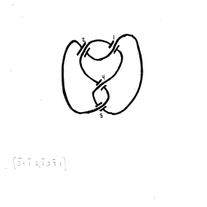
Figure 7: $4_{1}$ knot

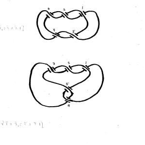
Figure 8: $5_{1}$ $5_{2}$ knots

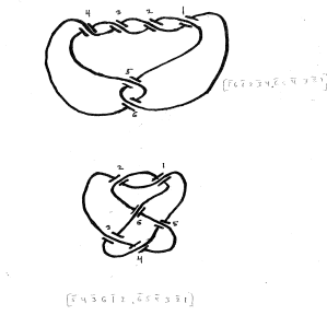
Figure 9: $6_{1}$ $6_{2}$ knots

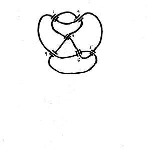
Figure 10: $6_{3}$ knot

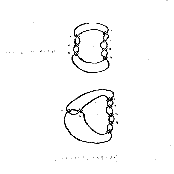
Figure 11: $7_{1}$ $7_{2}$

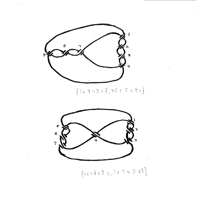
Figure 12: $7_{3}$ $7_{4}$

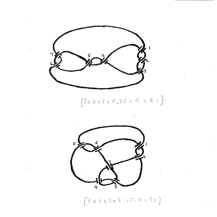
Figure 13: $7_{5}$ $7_{6}$

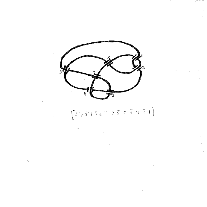
Figure 14: $7_{7}$