Fast and Accurate Frequency Estimation Using Sliding DFT

Abstract

Frequency Estimation of a complex exponential is a problem relevant to a large number of fields. In this paper a computationally efficient and accurate frequency estimator is presented using the guaranteed stable Sliding DFT which gives stability as well as computational efficiency. The estimator approaches Jacobsen s estimator and Candan s estimator for large N with an extra correction term multiplied to it for the stabilization of the sliding DFT. Simulation results show that the performance of the proposed estimator were found to be better than Jacobsen s estimator and Candan s estimator.

Index terms : Frequency Estimation, Sliding DFT, Radar Signal Processing

I Introduction

The frequency estimation of a complex sinusoid is a fundamental signal processing problem which finds a lot of importance in fields like radar signal processing.In radar signal processing the computational capability not only needs to be accurate but also fast which involves estimating the frequency every second. The received signal is corrupted by white gaussian noise. The best coarse frequency estimation of the signal is from the peak of the N point DFT of the received signal. A N point DFT is typically calculated for a data length of N samples which gives a resolution of $\frac{2\pi}{N}$. For real time spectral analysis a well known computationally efficient method is the sliding DFT especially in the cases when a new DFT spectrum is needed every few samples.The sliding DFT is computationally efficient than the radix-2 FFT. The sliding DFT performs a N point DFT within a sliding window of N samples.The window is then shifted by a sample for the next iteration and a new N point DFT is calculated which utilises the old N point DFT values.The single bin SDFT algorithm is implemented as an IIR filter, to which a comb filter can be added so as to compute all N DFT spectral components.In practical applications the algorithm can be initialised with zero input and zero output.The output wont be valid until N samples have been processed. The sliding DFT though has a marginally stable transfer function because all its poles lie on the z-domain’s unit circle.The filter coefficient numerical rounding might force the poles outside of the unit circle which results in instablity.A damping factor r may be used to force the pole into a radius of r inside the unit circle which guarantees stability.But the value of the bins obtained from the guaranteed stable sliding DFT are different from that of the traditional N point DFT.So the main problem lies in a fine estimation of frequency from the guaranteed stable sliding DFT which differ from the traditional N point DFT. The fine frequency estimation generally follows the coarse frequency estimation which is in turn done from the N point DFT.But the resolution of this process depends on the spacing of points taken for the fine resolution.In [3]-[6] the fine resolution estimate is done through a function on the DFT bins estimated from coarse resolution frequency estimaton.In [7] a simple relation for DFT interpolation is used and in [8] a bias correction is provided for [7].In this paper we derive Jacobsen’s formula for the guaranteed stable sliding DFT for which a bias correction term is also derived which includes bias correction for the damping factor r as well.

II problem description

A single complex sinusoid with white gaussian noise can be represented in the form

$$r[n]=Ae^{jwn}+w[n]$$

where A and $\omega$ are unknown variables which represent the amplitude and frequency of the complex sinusoid respectively where $\omega$=$\frac{2\pi(k_{p}+\delta)}{N}$ and $k_{p}$ is the index of the peak of the sliding DFT. $\delta$ is to be estimated from the three samples around the peak of the sliding DFT where $|\delta|$ $<$ 1/2

The transfer function for N point sliding DFT filter can be represented as

$$H(z)=\frac{1-r^{N}z^{-N}}{1-re^{j2k\pi/N}z^{-1}}$$

where $|r|<$ 1 Therefore a particular output bin of sliding DFT is written as

$$R[k]=\sum\limits_{n=0}^{N-1}x[n]r^{n}e^{-j2kn\pi/N}$$

where $|r|<$ 1 In practice though a particular output bin can be found out using the following recursive relation which basically serves the computational efficiency purpose

$$R_{k}[n]=R_{k}[n-1]re^{j2k\pi/N}-x(n-N)r^{N}+x(n)$$

The sliding DFT bin where the peak occurs and its immediate neighbours can be represented as follows:- Let the indices for the peak be $k_{p}$ and that of its immediate neighbours be $k_{p}-1$ and $k_{p}+1$ respectively.

$$R[k_{p}]=A\sum\limits_{n=0}^{N-1}r^{n}e^{j\frac{2\pi}{N}\delta n}+\hat{w}[k_{p}]$$

$$=Af(\delta)+\hat{w}[k_{p}]$$

(1)

$$R[k_{p}-1]=A\sum\limits_{n=0}^{N-1}r^{n}e^{j\frac{2\pi}{N}(\delta+1)n}+\hat{w}[k_{p}-1]$$

$$=Af(\delta+1)+\hat{w}[k_{p}-1]$$

(2)

$$R[k_{p}+1]=A\sum\limits_{n=0}^{N-1}r^{n}e^{j\frac{2\pi}{N}(\delta-1)n}+\hat{w}[k_{p}+1]$$

$$=Af(\delta-1)+\hat{w}[k_{p}+1]$$

(3)

where $\hat{w}[k]$ is the DFT of w[n] which also is white and

$$f(\alpha)=\sum\limits_{n=0}^{N-1}r^{n}e^{j\frac{2\pi}{N}\alpha n}$$

.

Our aim is to estimate the value of $\delta$ from these three samples $R[k_{p}]$,$R[k_{p}-1]$ and $R[k_{p}+1]$ so that

$$\hat{\omega}=2\pi/N(k_{p}+\delta)$$

becomes the fine frquency estimate. The two stage process consists of finding $k_{p}$ in the first stage and $\delta$ in the second stage.

III proposed estimator

To determine $\delta$ from the set of three equations we consider the Geometric Progression sums of each of the DFT bin and solve for $\delta$ using the approximation that the second and higher powers of $\delta$ are negligible as compared to $\delta$. We basically exploit the Geometric Progression sum in this case because of the added damping factor $r$ which in turn satisfies the relation $|r|<$ 1 and thus makes the common ratio in the Geometric Progression to be less than one.

$$f(\alpha)=\sum\limits_{n=0}^{N-1}r^{n}e^{j\frac{2\pi}{N}\alpha n}$$

$$=\frac{1-r^{N}}{1-re^{j\frac{2\pi\alpha}{N}}}$$

where $|r|<$ 1 To estimate $\delta$ We evaluate the first difference and second difference of $f(\delta)$ For evaluting the first and second differences which are $f(\delta+1)-f(\delta-1)$ and $f(\delta+1)-2f(\delta)+f(\delta-1)$ respectively (1) is used. Using elementary trigonometry the first difference

$$f(\delta+1)-f(\delta-1)$$

$$=\frac{1-r^{N}}{1-re^{j\frac{2\pi(\delta+1)}{N}}}-\frac{1-r^{N}}{1-re^{j\frac{2\pi(\delta-1)}{N}}}$$

which can be further simplified to

$$=\frac{2jr\sin(2\pi/N)e^{j2\pi\delta/N}(1-r^{N})}{1+r^{2}e^{j4\pi\delta/N}-2re^{j2\pi\delta/N}\cos(2\pi/N)}$$

Using elementary trigonometry the second difference

$$f(\delta+1)-2f(\delta)+f(\delta-1)$$

$$=\frac{1-r^{N}}{1-re^{j\frac{2\pi(\delta+1)}{N}}}-\frac{2(1-r^{N})}{1-re^{j\frac{2\pi\delta}{N}}}+\frac{1-r^{N}}{1-re^{j\frac{2\pi(\delta-1)}{N}}}$$

$$=\frac{(1-r^{N})(re^{j\frac{2\pi\delta}{N}}(e^{j\frac{\pi}{N}}-e^{-j\frac{\pi}{N}})^{2}+r^{2}e^{j\frac{4\pi\delta}{N}}(e^{j\frac{\pi}{N}}-e^{-j\frac{\pi}{N}})^{2})}{(1+r^{2}e^{j4\pi\delta/N}-2re^{j2\pi\delta/N}\cos(2\pi/N))(1-re^{j2\pi\delta/N})}$$

We get the following relation for the ratio of the two differences

$$\frac{f(\delta+1)-f(\delta-1)}{f(\delta+1)-2f(\delta)+f(\delta-1)}$$

$$=\frac{-j\cot(\pi/N)(1-r^{2}-2jr\sin(2\pi\delta/N))}{1+r^{2}+2r\cos(2\pi\delta/N)}$$

For large N and $\delta^{2}<<$1 we use the following approximations $\sin(2\pi\delta/N)=2\pi\delta/N$ and $\cos(2\pi\delta/N)=1$ the above relationship can be simplified to

$$=\frac{-j\cot(\pi/N)(1-r^{2}-4jr\pi\delta/N)}{(1+r)^{2}}$$

$$=-\frac{4\pi r\delta\cot(\pi/N)}{N(1+r)^{2}}-\frac{j(1-r^{2})\cot(\pi/N)}{(1+r)^{2}}$$

Simplifying the above relationship further we get

$$Real[\frac{f(\delta+1)-f(\delta-1)}{f(\delta+1)-2f(\delta)+f(\delta-1)}]$$

$$=-\frac{4\pi r\delta\cot(\pi/N)}{N(1+r)^{2}}$$

(4) Thus an estimate of $\delta$ can be produced by the substitution of $f(\delta)\dashrightarrow R[k_{p}],f(\delta-1)\dashrightarrow R[k_{p}+1]$ and $f(\delta+1)\dashrightarrow R[k_{p}-1]$ (which were inturn derived in the relations (1),(2) and (3)) in (4);

$$\hat{\delta}=\frac{(1+r)^{2}}{4r}\frac{\tan(\pi/N)}{\pi/N}Real[\frac{R[k_{p}-1]-R[k_{p}+1]}{2R[k_{p}]-R[k_{p}-1]-R[k_{p}+1]}]$$

IV Numerical Comparisons

In this section we present a numerical comparison between the proposed estimator and the other estimators namely, Candace’s estimator and Jacobsen’s estimator.The performance of the proposed estimator is compared across various damping factors which is shown in Fig. 1. The simulation is done in MATLAB.A sinusoidal signal is taken whose frequency is varied from 30.1 MHz to 30.9 MHz in steps of 0.1 MHz. 128 samples of the signal are taken where the sampling frequency is 128 MHz.A 128 point sliding DFT is taken for the proposed estimator while a 128 point traditional DFT is taken for the other estimators.The noise taken is white gaussian noise.

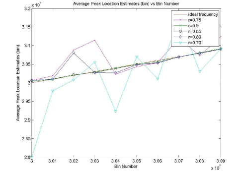
Figure 1: Performance of the proposed estimator with different damping factors

Fig. 2 shows the bias values of the proposed estimator and the other estimators with respect to the ideal frequency in the absence of noise for $\emph{N}=$128.This shows that none of the estimators are unbiased.For the proposed estimator the damping factor taken is $\emph{r}=$0.9 for the simulations.It can be clearly seen that the bias of the proposed estimator is less than 1000 Hz while those of the other estimators have higher bias values.

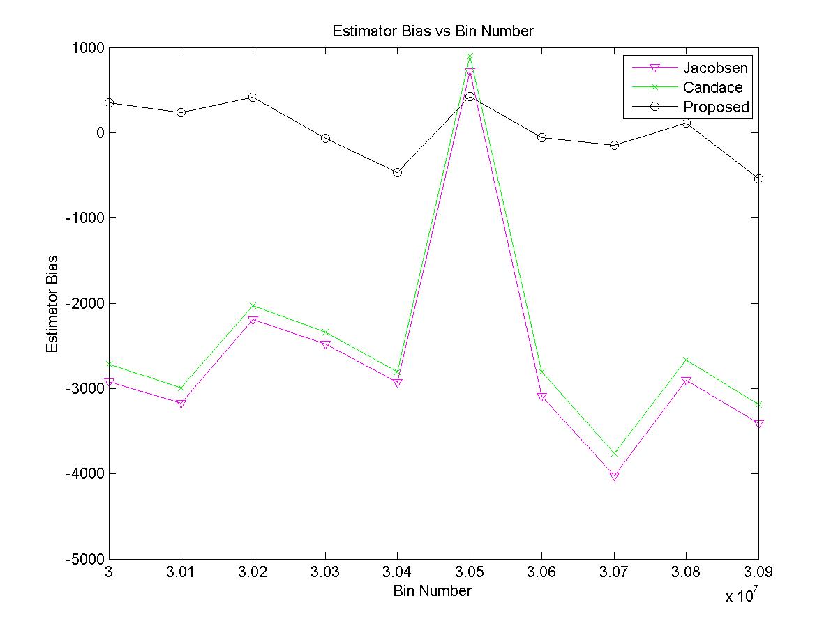
Figure 2: Variation of bias of different estimators in absence of noise

Fig. 3 shows the performance of the proposed estimator and the other estimators with respect to ideal frequency is presence of noise for $\emph{N}=$128.

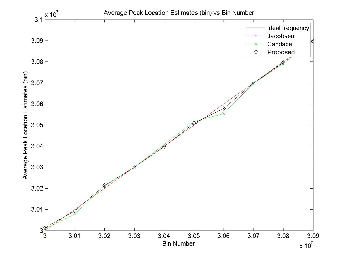
Figure 3: Performance of the estimators in presence of noise

Fig. 4 examines the bias of the estimators in presence of noise.It can be seen that the proposed estimator has lower bias as compared to the other estimators.With higher SNR values the bias values in presence of noise approach the bias values in absence of noise.

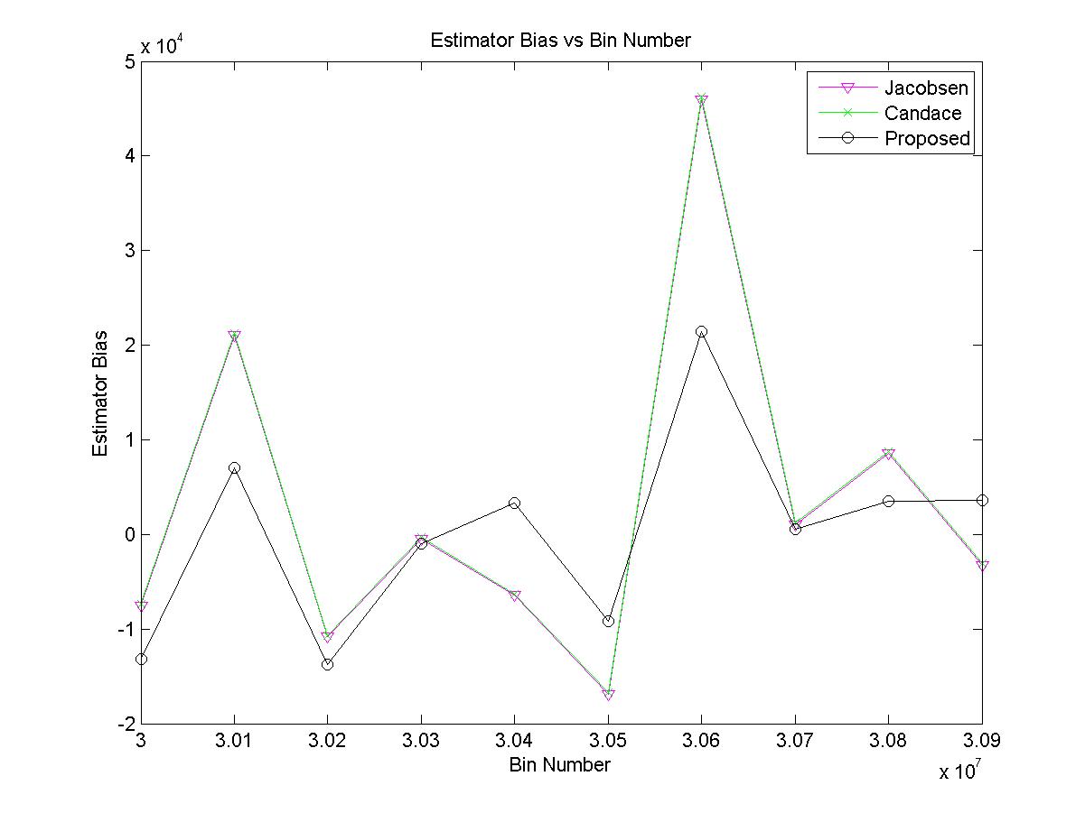
Figure 4: Variation of bias of different estimators in presence of noise

Fig. 5 examines the RMSE values of the estimators for large number of observations.

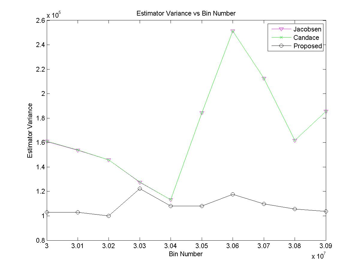
Figure 5: Variation of RMSE of different estimators in presence of noise

The SNR values taken for the above simulations range from 2 dB to 3dB. At higher SNR values the estimator bias and the variance values decrease further and all the three estimators behave nearly the same with the proposed estimator giving even lower bias and variance values. It should be noted that with the damping factor r approaching 1 with higher values of N the proposed estimator have nearly the same performance.The value of the damping factor has been kept around 0.9 for guaranteed stability and better performance.It is intutively satisfying that the bias correction factor in Candace’s estimator is also a part of the derived expression for the proposed estimator.The fewer number of operations involved for the proposed estimator compared to that of other estimators and the lower bias and variance values makes the proposed estimator very useful for radar signal processing.

V Conclusions

A new estimator is proposed which requires very few number of operations per output sample.The estimator has a correction term for bias.The good performance of the estimator is justified in the paper.The proposed estimator has low bias and variance values which makes it a really valuable tool in the field of radar signal processing. Simulation results showing superiority of the proposed estimator is provided.

The present work revolves around accurately estimating a single tone frequency or a multi tone frequencies where the tones have large seperations.A potential future work is the extension of present work to accurately estimating multi tone frequencies which are closely seperated without increasing the number of computations.

References

- [1] M.A.Richards,Fundamentals of Radar Signal Processing, New York:McGraw Hill, 2005.
- [2] M.D.Macleod,”Fast nearly ML estimation of the parameters of real or complex single or complex single tones or resolved multiple tones,”IEEE Trans. Signal Process.,vol. 46,no. 1,pp. 141-148,Jan. 1998
- [3] E.Jacobsen and P.Kootsookos,”Fast Accurate Frequency Estimators,” IEEE Trans.Signal Process.,vol. 24,pp. 123-125,May 2007
- [4] C.Candan,”A Method for Fine Resolution Frequency Estimation from Three DFT Samples,”IEEE Signal Processing Letters.,vol. 18,pp. 351-354,April 2011
- [5] B.G.Quinn,”Estimating Frequency by interpolation using Fourier coefficients,” ”IEEE Trans.Signal Process.,vol. 42,no. 5,pp. 1264-1268,May 1994
- [6] B.G.Quinn,”Estimation of frequency,amplitude and phase from the DFT of a time series,” IEEE Trans.Signal Process.,vol. 45,no. 3,pp. 814-817,March 1997
- [7] E.Jacobsen and R.Lyons,”The sliding DFT,” IEEE Signal Processing Magazine.,vol. 20,no. 2,pp. 74-80,March 2003