Non-perturbation theory of electronic dynamic conductivity for two-barrier resonance
tunnel nano-structure

Abstract

The non-perturbation theory of electronic dynamic conductivity for open two-barrier resonance tunnel structure is established for the first time within the model of rectangular potentials and different effective masses of electrons in the elements of nano-structure and the wave function linear over the intensity of electromagnetic field. It is proven that the results of the theory of dynamic conductivity, developed earlier in weak signal approximation within the perturbation method, qualitatively and quantitatively correlate with the obtained results. The advantage of non-perturbation theory is that it can be extended to the case of electronic currents interacting with strong electromagnetic fields in open multi-shell resonance tunnel nano-structures, as active elements of quantum cascade lasers and detectors. resonance tunnel nano-structure, conductivity, non-perturbation theory 73.21.Fg, 73.90.+f, 72.30.+q, 73.63.Hs

Abstract

Вперше запропоновано непертурбацiйну теорiю електронної динамiчної провiдностi вiдкритої двобар’єрної резонансно-тунельної структури у моделi прямокутних потенцiалiв i рiзних ефективних мас електронiв у рiзних елементах наносистеми та з лiнiйною за напруженiстю електромагнiтного поля хвильовою функцiєю системи. Показано, що результати розвинутої ранiше теорiї динамiчної провiдностi у малосигнальному наближеннi (у межах теорiї збурень) якiсно i кiлькiсно корелюють з отриманими результатами. Переваги непертурбацiйної теорiї в тому, що вона може бути поширена на випадок взаємодiї потокiв електронiв з потужними електромагнiтними полями у вiдкритих багатошарових резонансно-тунельних наноструктурах, як активних елементах квантових каскадних лазерiв i детекторiв. резонансно-тунельна наноструктура, провiднiсть, непертурбацiйна теорiя

1 Introduction

The experimental produce of nano-lasers and nano-detectors and, further, quantum cascade lasers and detectors [1, 2, 3] stimulates the intensive development of the theory of dynamic conductivity for nano-heterosystems as active elements of these unique devices. In spite of the twenty years period of investigating the interaction between electromagnetic field and electronic currents in open nano-structures, the respective theory is far from being completed. One of the reasons is the mathematical problems arising at the quantum mechanical research of physical processes caused by the interaction of quasi-particles with classic and quantized (phonons) fields in open nano-structures.

The theory of electronic conductivity for the two- and three-barrier resonance tunnel structures (RTS) [4, 5, 6, 7, 8, 9, 10] is rather complicated and mathematically sophisticated even without taking into account the dissipative processes (scattering at the phonons, impurities, imperfections). Therefore, the maximally simplified model is used in the above mentioned and other papers [11, 12, 13]: $\delta$-like approximation of potential barriers for the electrons and weak signal approximation equivalent to the first order of perturbation theory (PT) over the intensity of electromagnetic field interacting with electronic current in RTS.

We must note that $\delta$-like approximation of potential barriers essentially simplifies the model of nano-structure. Herein, the electron is automatically characterized by the unitary effective mass within the whole system, which permits to calculate the RTS dynamic conductivity [4, 5, 6, 7, 8, 9, 10, 11, 12, 13] using the PT iteration method and in such a way, quit the frames of linear approximation over the field intensity.

Further, in references [14, 15] it was shown that $\delta$-like approximation of potential barriers correctly described the qualitative properties of spectral parameters of quasi-stationary states of electrons and the dynamic conductivity of nano-structures but the magnitudes of resonance energies were overestimated by tens per cent and resonance widths by ten times with respect to their magnitudes in a more realistic model of rectangular potentials and different effective masses of electron in the elements of nano-structure. It was displayed that in any RTS, the $\delta$-barrier model strongly underestimated the electrons life times in all quasi-stationary states and, thus, the magnitude of the dynamic conductivity became the orders smaller even for the structures with weak electromagnetic field.

The theory of dynamic conductivity established in references [16, 17, 18, 19] for the open two- and three-barrier RTS is based, as a rule, on a more realistic model but it is so complicated compared to the $\delta$-barrier model that it is practically impossible to leave the framework of weak signal approximation. Nevertheless, the development of experimental capabilities makes the problem of strong interaction of electronic currents and electromagnetic field in RTS more and more urgent.

Therefore, it is necessary to develop the non-perturbation theory (NPT) of conductivity for open RTS where the intensity of electromagnetic field would not play such a critical role as in PT. The motivation for the positive expectations regarding the NPT existed because the solution of complete Schrodinger equation with Hamiltonian describing the interaction between electrons and varying in time electromagnetic field was known [20]. However, in spite of the known analytical expression for the exact wave function, the theory of conductivity for the open RTSs was not successfully developed.

The possible approach to the solution of this problem for the dynamic conductivity of the two-barrier RTS is proposed in our paper for the first time. We develop the NPT for the electronic dynamic conductivity using the wave function which is the exact solution of complete Schrodinger equation in the linear approximation over the field. Being convinced that the results obtained in the first order of PT for electronic conductivity correlate with the results of the herein developed NPT, the established approach can be used in developing a general theory of electronic current interacting with strong electromagnetic field in open multi-shell nano-structures, being the active elements of quantum cascade lasers and detectors.

2 Hamiltonian of the system. Finding the wave function from the complete Schrodinger equation

The open two-barrier RTS is studied in the Cartesian coordinate system with OZ axis perpendicular to the planes of nano-structure, figure 1. The small difference between the lattice constants of the nano-structure wells and barriers makes it possible to use the effective masses

$$m(z)=m_{0}\sum\limits_{p=0}^{2}[\theta(z-z_{2p-1})-\theta(z-z_{2p})]+m_{1}\sum\limits_{p=0}^{1}[\theta(z-z_{2p})-\theta(z-z_{2p+1})]$$ (1)

and rectangular potentials

$$U(z)=U\sum\limits_{p=0}^{1}[\theta(z-z_{2p})-\theta(z-z_{2p+1})].$$ (2)

Here $\theta(z)$ is Heaviside step function; $z_{-1}\rightarrow-\infty$, $z_{4}\rightarrow+\infty$.

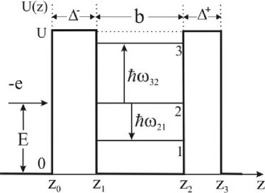
Figure 1: Energy scheme for the electrons and geometry of two-barrier RTS.

It is assumed that mono-energetic electron current with the energy ($E$), density of current ($J_{0}^{+}\sim\sqrt{E}$) and concentration ($n_{0}$) moving perpendicularly to the planes of two-barrier RTS falls at it from the left side. The electronic movement can be considered as one-dimensional ($\overrightarrow{k}_{||}=0$). According to the numeric evaluations, the velocity within the nano-structure is by 3–4 orders smaller than the velocity outside. Thus, the interaction between electrons and electromagnetic field with frequency ($\omega$) and intensity of electric field ($\epsilon$) is essential only within the two-barrier RTS and can be neglected outside it.

The electron wave function has to satisfy the complete Schrodinger equation

$$\mathrm{i}\hbar\frac{\partial\Psi(E,\omega,z,t)}{\partial t}=[H_{0}(z)+H_{1}(z,t)]\Psi(E,\omega,z,t),$$ (3)

where

$$H_{0}(z)=-\frac{\hbar^{2}}{2}\frac{\partial}{\partial z}\frac{1}{m(z)}\frac{\partial}{\partial z}+U(z)$$ (4)

is the Hamiltonian of the electron without interaction with the field.

The electron interaction with the electromagnetic field varying in time, is described by the Hamiltonian

$$H_{1}(z,t)=-2e\epsilon z[\theta(z)-\theta(z-z_{3})]\cos\omega t.$$ (5)

The both linearly independent exact solutions of complete Schrodinger equation with Hamiltonian $H_{0}(z)$ in the potential well are known: $\exp(\pm\mathrm{i}kz-\mathrm{i}\omega_{0}t)$ [17, 19], $\omega_{0}=E\hbar^{-1}$. The both linearly independent exact solutions of equation (3) with Hamiltonian $H(z,t)=H_{0}(z)+H_{1}(z,t)$, taking into account the electron-electromagnetic field interaction in linear approximation over the electric intensity are also known:

$$\exp\left[\mathrm{i}\left(\pm kz-\omega_{0}t+\frac{2e\epsilon z}{\hbar\omega}\sin\omega t\pm\frac{2e\epsilon k}{m\omega^{2}}\cos\omega t\right)\right],$$

where $k$ is electron quasi-momentum [20]. Thus, using the exact solutions of equation (3) for the case of two-barrier RTS, the electron wave function is written as

$$\Psi(E,\omega,z,t)=\Psi_{0}(E,z,t)\theta(-z)+\sum\limits_{p=1}^{3}\Psi_{p}(E,\omega,z,t)[\theta(z-z_{p-1})-\theta(z-z_{p})]+\Psi_{4}(E,z,t)\theta(z-z_{3}).$$ (6)

In the outer media of two-barrier RTS, where the interaction with electromagnetic field is neglected, the wave functions are

$$\Psi_{0}(E,z,t)=(a_{0}\mathrm{e}^{\mathrm{i}kz}+b_{0}\mathrm{e}^{-\mathrm{i}kz})\mathrm{e}^{-\mathrm{i}\omega_{0}t},$$ (7)

$$\Psi_{4}(E,z,t)=a_{4}\mathrm{e}^{\mathrm{i}kz-\mathrm{i}\omega_{0}t},$$ (8)

where

$$k=\hbar^{-1}\sqrt{2m_{0}E}\,.$$

Here it is taken into account that the mono-energetic electronic current impinges at RTS from the left hand side, since in the left hand media there is both a falling and a reflected wave while in the right one there is the wave moving towards the infinity only.

Within the two-barrier RTS, where the electron-electromagnetic field interaction is essential, the wave function is found as linear combinations of eigen wave functions of the Hamiltonian $H(z,t)$

$$\Psi_{1}(E,\omega,z,t) =\left[a_{1}f_{1}^{\rightarrow}(E,\omega,z,t){\re}^{\chi z}+b_{1}f_{1}^{\leftarrow}(E,\omega,z,t)\mathrm{e}^{-\chi z}\right]\mathrm{e}^{-\mathrm{i}\omega_{0}t}$$

$$\Psi_{2}(E,\omega,z,t) =\left[a_{2}f_{2}^{\rightarrow}(E,\omega,z,t)\mathrm{e}^{\mathrm{i}kz}+b_{2}f_{2}^{\leftarrow}(E,\omega,z,t)\mathrm{e}^{-\mathrm{i}kz}\right]\mathrm{e}^{-\mathrm{i}\omega_{0}t},$$ (9)

$$\Psi_{3}(E,\omega,z,t) =\left[a_{3}f_{1}^{\rightarrow}(E,\omega,z,t)\mathrm{e}^{\chi z}+b_{3}f_{1}^{\leftarrow}(E,\omega,z,t)\mathrm{e}^{-\chi z}\right]\mathrm{e}^{-\mathrm{i}\omega_{0}t},$$ (10)

where

$$f_{p}^{\rightleftarrows}(E,\omega,z,t)=\exp(\mathrm{i}\alpha\sin\omega t\pm\mathrm{i}\beta_{p}\cos\omega t)\ ,\quad\quad(p=1,2)$$ (11)

$$\alpha=\frac{2e\epsilon z}{\hbar\omega}\,;\quad\quad\beta_{1}=\frac{2\mathrm{i}e\epsilon\chi}{m_{1}\omega^{2}}\,;\quad\quad\beta_{2}=\frac{2e\epsilon k}{m_{0}\omega^{2}}\,;\quad\quad\chi=\hbar^{-1}\sqrt{2m_{1}(U-E)}\,.$$ (12)

Further, using the known [21] expansion of exponential functions into Fourier range over all the harmonics, the functions $f_{p}^{\rightleftarrows}(E,\omega,z,t)$ are written as

$$f_{p}^{\rightleftarrows}(E,\omega,z,t)=\sum\limits_{n_{1}=-\infty}^{\infty}\sum\limits_{n_{2}=-\infty}^{\infty}\mathrm{i}^{\pm n_{2}}j_{n_{1}}(\alpha)j_{n_{2}}(\beta_{p})\mathrm{e}^{\mathrm{i}(n_{1}\mp n_{2})\omega t}\ ,$$ (13)

where $j_{n}$ are the cylindrical Bessel functions of the whole order.

The quantum transitions, accompanied by energy radiation or absorption, occur between electron quasi-stationary states with odd number under the effect of electromagnetic field. The most intensive transitions arise between the neighbouring resonance states. Thus, the expression (13) for the functions $f_{p}^{\rightleftarrows}(E,\omega,z,t)$ can be essentially simplified by leaving only zero and first harmonics from the whole infinite range. Then, in a one-mode approximation for the functions $f_{p}^{\rightleftarrows}(E,\omega,z,t)$, the following expression is obtained

$$f_{p}^{\rightleftarrows}(E,\omega,z,t) = C_{p}^{\rightleftarrows}(E,\omega,z)+\left\{D_{p}(E,\omega,z)+\mathrm{i}\left[F_{p}^{\rightleftarrows}(E,\omega,z)+G_{p}^{\rightleftarrows}(E,\omega,z)\right]\right\}\mathrm{e}^{-\mathrm{i}\omega t}$$ (14)

$$+ \left\{-D_{p}(E,\omega,z)+\mathrm{i}\left[F_{p}^{\rightleftarrows}(E,\omega,z)-G_{p}^{\rightleftarrows}(E,\omega,z)\right]\right\}\mathrm{e}^{\mathrm{i}\omega t},$$

with

$$C_{p}^{\rightleftarrows}(E,\omega,z)=j_{0}(\alpha)j_{0}(\beta_{p})+2\sum\limits_{n_{1}=1}^{\infty}[j_{4n_{1}}(\alpha)j_{4n_{1}}(\beta_{p})-j_{4n_{1}-2}(\alpha)j_{4n_{1}-2}(\beta_{p})],$$ (15)

$$D_{p}(E,\omega,z)=\sum\limits_{n_{1}=1}^{\infty}\{j_{4n_{1}-1}(\alpha)[j_{4n_{1}}(\beta_{p})+j_{4n_{1}-2}(\beta_{p})]-j_{4n_{1}-3}(\alpha)[j_{4n_{1}-2}(\beta_{p})+j_{4n_{1}-4}(\beta_{p})]\},$$ (16)

$$G_{p}^{\rightleftarrows}(E,\omega,z)=\pm\sum\limits_{n_{1}=1}^{\infty}\{j_{4n_{1}}(\alpha)[j_{4n_{1}-1}(\beta_{p})-j_{4n_{1}+1}(\beta_{p})]+j_{4n_{1}-2}(\alpha)[j_{4n_{1}-1}(\beta_{p})-j_{4n_{1}-3}(\beta_{p})]\}.$$ (17)

Within the framework of the linear Hamiltonian over the field intensity ($\epsilon$), the rather complicated formulas (15)–(17) correctly define the electron wave function in a one-mode approximation independently of the intensity magnitude. In the case of small intensity when the condition

$$\min[\alpha(E),\beta_{1}(E),\beta_{2}(E)]\ll 1$$ (18)

is fulfilled, expanding the Bessel functions into a series and preserving the linear term over the field, the expressions for coefficients are simplified

$$C_{p}^{\rightleftarrows}=1;\quad\quad\quad D_{p}=-\alpha/2;\quad\quad\quad F_{p}^{\rightleftarrows}=\pm\beta_{p}/2;\quad\quad\quad G_{p}^{\rightleftarrows}=0.$$ (19)

Thus, the wave function is also obtained in a convenient analytical form

$$\Psi(E,\omega,z,t)\! = \!(a_{0}\mathrm{e}^{\mathrm{i}kz}+b_{0}\mathrm{e}^{-\mathrm{i}kz})\mathrm{e}^{-\mathrm{i}\omega_{0}t}\theta(-z)+a_{4}\mathrm{e}^{\mathrm{i}kz}\mathrm{e}^{-\mathrm{i}\omega_{0}t}\theta(z-z_{3})$$ (20)

$$+ \!\sum\limits_{p=1}^{3}\mathrm{e}^{-\mathrm{i}\omega_{0}t}\left\{a_{p}\mathrm{e}^{K_{p}z}\left[1+\frac{1}{2}(\mathrm{i}\beta_{p}+\alpha)\mathrm{e}^{\mathrm{i}\omega t}+\frac{1}{2}(\mathrm{i}\beta_{p}-\alpha)\mathrm{e}^{-\mathrm{i}\omega t}\right]\right.$$

$$+ \!\left.b_{p}\mathrm{e}^{-K_{p}z}[1-\frac{1}{2}(\mathrm{i}\beta_{p}-\alpha)\mathrm{e}^{\mathrm{i}\omega t}-\frac{1}{2}(\mathrm{i}\beta_{p}+\alpha)\mathrm{e}^{-\mathrm{i}\omega t}]\right\}\left[\theta(z-z_{p-1})-\theta(z-z_{p})\right],\quad$$

where

$$K_{1}=K_{3}=\chi;\quad\quad\quad K_{2}=\mathrm{i}k.$$

Using the obtained wave function $\Psi(E,\omega,z,t)$ one can perform the calculation of the permeability coefficient for the two-barrier RTS, obtaining the spectral parameters of electron quasi-stationary states and active dynamic conductivity of nano-structure.

3 Permeability coefficient and dynamic conductivity of two-barrier RTS

Now, we can find the dynamic conductivity caused by the quantum transitions of electrons from the quasi-stationary state with the energy $E$ into the states with the energies $E+\hbar\omega$ or $E-\hbar\omega$ due to the effect of the periodical electromagnetic field with intensity $\epsilon$ and frequency $\omega$. Therefore, we have to define the densities of electron currents: $J(E+\hbar\omega)$ and $J(E-\hbar\omega)$, flowing out of the RTS with the respective energies. In such approach, the complete wave function is written as linear combination of wave functions describing the electron states with the energies $E$, $E+\hbar\omega$ and $E-\hbar\omega$. The functions $\Psi(E\pm\hbar\omega,\omega,z,t)$ can be obtained from the expression (20) for the already known function $\Psi(E,\omega,z,t)$ using the substitution $E\rightarrow E\pm\hbar\omega$. Then,

$$\Psi(E\pm\hbar\omega,\omega,z,t) = b_{0}^{\pm}\mathrm{e}^{-\mathrm{i}k^{\pm}z}\mathrm{e}^{-\mathrm{i}(\omega_{0}\pm\omega)t}\theta(-z)+a_{4}^{\pm}\mathrm{e}^{\mathrm{i}k^{\pm}z}\mathrm{e}^{-\mathrm{i}(\omega_{0}\pm\omega)t}\theta(z-z_{3})$$ (21)

$$+ \sum\limits_{p=1}^{3}\mathrm{e}^{-\mathrm{i}\omega_{0}t}\left\{a_{p}^{\pm}\mathrm{e}^{K_{p}^{\pm}z}\left[\mathrm{e}^{\mp\mathrm{i}\omega t}+\frac{1}{2}(\mathrm{i}\beta_{p}^{\pm}\pm\alpha)+\frac{1}{2}(\mathrm{i}\beta_{p}^{\pm}\mp\alpha)\mathrm{e}^{\mp 2\mathrm{i}\omega t}\right]\right.$$

$$+ \left.b_{p}^{\pm}\mathrm{e}^{-K_{p}^{\pm}z}\left[\mathrm{e}^{\mp\mathrm{i}\omega t}-\frac{1}{2}(\mathrm{i}\beta_{p}^{\pm}\mp\alpha)-\frac{1}{2}(\mathrm{i}\beta_{p}^{\pm}\pm\alpha)\mathrm{e}^{\mp 2\mathrm{i}\omega t}\right]\right\}$$

$$\times \left[\theta(z-z_{p-1})+\theta(z-z_{p})\right],$$

where

$$K_{1}^{\pm}=K_{3}^{\pm}=\chi^{\pm}=\hbar^{-1}\sqrt{2m_{1}[U-(E\pm\hbar\omega)]}\,;\quad K_{2}^{\pm}=\mathrm{i}k^{\pm}=\mathrm{i}\hbar^{-1}\sqrt{2m_{0}(E\pm\hbar\omega)}\,;$$ (22)

$$\beta_{1}^{\pm}=\frac{2\mathrm{i}e\epsilon\chi^{\pm}}{m_{1}\omega^{2}}\,;\qquad\beta_{2}^{\pm}=\frac{2e\epsilon k^{\pm}}{m_{0}\omega^{2}}\,.$$ (23)

The mono-energetic electron current falls at RTS with the energy $E=\hbar\omega_{0}$. Under the effect of electromagnetic field there occur quantum transitions into higher (with the energy $E+\hbar\omega$) or lower (with the energy $E-\hbar\omega$) electron quasi-stationary states, the currents from which produce the dynamic conductivity of a nano-structure. In order to describe this physical process correctly, we have to leave the terms containing only the first harmonic ($\pm\omega$) in formula (21) for the wave function. Thus,

$$\Psi(E\pm\hbar\omega,\omega,z,t) = b_{0}^{\pm}\mathrm{e}^{-\mathrm{i}k^{\pm}z}\mathrm{e}^{-\mathrm{i}(\omega_{0}\pm\omega)t}\theta(-z)+a_{4}^{\pm}\mathrm{e}^{\mathrm{i}k^{\pm}z}\mathrm{e}^{-\mathrm{i}(\omega_{0}\pm\omega)t}\theta(z-z_{3})$$ (24)

$$+ \sum\limits_{p=1}^{3}\mathrm{e}^{-\mathrm{i}(\omega_{0}\pm\omega)t}(a_{p}^{\pm}\mathrm{e}^{K_{p}^{\pm}z}+b_{p}^{\pm}\mathrm{e}^{-K_{p}^{\pm}z})[\theta(z-z_{p-1})+\theta(z-z_{p})].$$

The complete wave function $\Phi(E,E-\hbar\omega,E+\hbar\omega,\omega,z,t)$ can be written at the base of superposition (linear combination) of wave functions (20) and (24). It depends on electron energies $E$, $E-\hbar\omega$, $E+\hbar\omega$ and electromagnetic field frequency $\omega$. For a convenient presentation, it is further written as $\Phi(E,\omega,z,t)$.

$$\Phi(E,\omega,z,t) = \Phi_{0}(E,\omega,z,t)\theta(-z)$$ (25)

$$+ \sum\limits_{p=1}^{3}\Phi_{p}(E,\omega,z,t)[\theta(z-z_{p-1})-\theta(z-z_{p})]+\Phi_{4}(E,\omega,z,t)\theta(z-z_{3}),$$

where

$$\Phi_{0}(E,\omega,z,t) =\mathrm{e}^{-\mathrm{i}\omega_{0}t}\left(A_{0}\mathrm{e}^{\mathrm{i}kz}+B_{0}\mathrm{e}^{-\mathrm{i}kz}+B_{0}^{+}\mathrm{e}^{-\mathrm{i}k^{+}z}\mathrm{e}^{-\mathrm{i}\omega t}+B_{0}^{-}\mathrm{e}^{-\mathrm{i}k^{-}z}\mathrm{e}^{\mathrm{i}\omega t}\right),$$ (26)

$$\Phi_{p}(E,\omega,z,t) =\mathrm{e}^{-\mathrm{i}\omega_{0}t}\left\{A_{p}\mathrm{e}^{K_{p}z}\left[1+\frac{1}{2}(\mathrm{i}\beta_{p}+\alpha)\mathrm{e}^{\mathrm{i}\omega t}+\frac{1}{2}(\mathrm{i}\beta_{p}-\alpha)\mathrm{e}^{-\mathrm{i}\omega t}\right]\right.$$

$$+B_{p}\mathrm{e}^{-K_{p}z}\left[1-\frac{1}{2}(\mathrm{i}\beta_{p}-\alpha)\mathrm{e}^{\mathrm{i}\omega t}-\frac{1}{2}(\mathrm{i}\beta_{p}+\alpha)\mathrm{e}^{-\mathrm{i}\omega t}\right]$$

$$+\left.\left(A_{p}^{+}\mathrm{e}^{K_{p}^{+}z}+B_{p}^{+}\mathrm{e}^{-K_{p}^{+}z}\right)\mathrm{e}^{-\mathrm{i}\omega t}+\left(A_{p}^{-}\mathrm{e}^{K_{p}^{-}z}+B_{p}^{-}\mathrm{e}^{-K_{p}^{-}z}\right)\mathrm{e}^{\mathrm{i}\omega t}\right\},$$ (27)

$$\Phi_{4}(E,\omega,z,t) =\mathrm{e}^{-\mathrm{i}\omega_{0}t}\left(A_{4}\mathrm{e}^{\mathrm{i}kz}+A_{4}^{+}\mathrm{e}^{\mathrm{i}k^{+}z}\mathrm{e}^{-\mathrm{i}\omega t}+A_{4}^{-}\mathrm{e}^{\mathrm{i}k^{-}z}\mathrm{e}^{\mathrm{i}\omega t}\right).$$ (28)

The two-barrier RTS under study is an open one, consequently the wave function $\Phi(E,\omega,z,t)$ at any moment of time has to satisfy the normality condition

$$\int\limits_{-\infty}^{\infty}\Phi^{*}(k^{\prime},\omega,z,t)\Phi(k,\omega,z,t)\mathrm{d}z=\delta(k-k^{\prime}).$$ (29)

The wave function and its density of current should be continuous at all nano-structure interfaces

$$\Phi_{p}(E,\omega,z_{p},t)=\Phi_{p+1}(E,\omega,z_{p},t);\quad\quad\frac{\partial\Phi_{p}(E,\omega,z,t)}{m_{0(1)}\ \partial z}\bigg{|}_{z=z_{p}}=\frac{\partial\Phi_{p+1}(E,\omega,z,t)}{m_{1(0)}\ \partial z}\bigg{|}_{z=z_{p}}.$$ (30)

The coefficients at zero harmonics: $B_{0},A_{p},B_{p},A_{4}$ are definitely obtained from the system of homogeneous equations (30) through the coefficient $A_{0}$. This is, in turn, related to the density of start electron current impinging at RTS: $J_{0}^{+}=en_{0}\sqrt{2Em_{0}^{-1}}|A_{0}|^{2}$, where $n_{0}$ is the concentration of electrons in this current, $e$ is electron charge. Coefficients at the first harmonics: $B_{0}^{\pm},A_{p}^{\pm},B_{p}^{\pm},A_{4}^{\pm}$ are defined through the now known coefficients at zero harmonics of function $\Phi(E,\omega,z,t)$. According to the quantum mechanics [22], the permeability coefficient for the two-barrier RTS is

$$D(E)=|A_{4}/A_{0}|^{2}.$$ (31)

It is well known [14, 23] that the permeability coefficient $D(E)$ determines the spectral parameters: resonance energies ($E_{n}$) and resonance widths ($\Gamma_{n}$) of quasi-stationary states of electrons. The positions of $D(E)$ maxima in the energy scale fix the resonance energies, while their widths at the halves of maximal heights $D(E_{n})$ fix the resonance widths of these quasi-stationary states.

According to electrodynamics [24], in a quasi-static approximation, the energy ($\mathcal{E}$), got by the electrons from the field during the period $T=2\pi/\omega$, is related to the real part of dynamic conductivity ($\sigma$)

$$\mathcal{E}=\frac{4\pi z_{3}\epsilon^{2}}{\omega}\sigma(E,\omega).$$ (32)

The same energy is defined by the electron currents flowing out of the nano-structure through the densities of currents of uncoupling electrons

$$\mathcal{E}=\frac{\hbar\omega T}{e}\left\{\left[J(E+\hbar\omega,z_{3})-J(E+\hbar\omega,0)\right]-\left[J(E-\hbar\omega,z_{3})-J(E-\hbar\omega,0)\right]\right\}.$$ (33)

According to quantum mechanics [22], the density of current is defined by the wave function $\Phi(E,\omega,z,t)$

$$J(E,z)=\frac{\mathrm{i}e\hbar n_{0}}{2m(z)}\left[\Phi(E,\omega,z,t)\frac{\partial\Phi^{*}(E,\omega,z,t)}{\partial z}-\Phi^{*}(E,\omega,z,t)\frac{\partial\Phi(E,\omega,z,t)}{\partial z}\right].$$ (34)

Thus, as a result of analytical calculations, the final expression for the dynamic conductivity of two-barrier RTS is obtained:

$$\sigma(E,\omega)=\frac{\hbar^{2}\omega n_{0}}{2z_{3}m_{0}\epsilon^{2}}[k^{+}(|B_{0}^{+}|^{2}+|A_{4}^{+}|^{2})-k^{-}(|B_{0}^{-}|^{2}+|A_{4}^{-}|^{2})]\ .$$ (35)

It is evident that in linear approximation over the electromagnetic field intensity, the coefficients $B_{0}^{\pm},A_{4}^{\pm}$ are also linear. Consequently, in this approximation, (the same in PT [4, 5, 6, 7, 8, 9, 10, 11, 12, 13, 15, 16, 17, 18, 19]) the dynamic conductivity is independent of $\epsilon$.

The calculations of spectral parameters of electron quasi-stationary states and dynamic conductivity of nano-structure were performed at the base of the developed NPT for In_0.52Al_0.48As/In_0.53Ga_0.47As two-barrier RTS with physical parameters: $m_{0}$ = 0.046 $m_{e}$, $m_{1}$ = 0.089 $m_{e}$, $U$ = 516 meV, $n_{0}$ = $10^{16}$ cm^-3 and typical geometrical ones: $b$ = 10.8 nm, $\Delta^{+}+\Delta^{-}$ = 6 nm, $\Delta^{+}$ = 2 $\div$ 4.5 nm. The same calculations were performed in the frames of the previously developed PT [19] in the first order over the field intensity for comparison.

The results obtained for positive or negative conductivities $\sigma(E,\Omega=\hbar\omega)$ produced by the quantum transitions of electrons interacting with electromagnetic field in the processes of absorption ($1\rightarrow 2$) or radiation ($2\rightarrow 1$) are shown in figures 2 (a), (b) and figures 2 (d), (e), respectively.

The spectral parameters (resonance energies and resonance widths) of electron quasi-stationary states, defined from the permeability coefficient [14, 23], do not depend on the method of calculation. Their magnitudes, obtained for the two-barrier RTS with $b$=10.8 nm, $\Delta^{+}=\Delta^{-}$=3 nm are presented in figures 2 (a), (b), (d), (e). The figures prove that the functions $\sigma(E,\Omega={\rm const})$ and $\sigma(E={\rm const},\Omega)$ are of the shape of Lorentz curve in both methods (NPT and PT). However, herein, it is clear that the magnitudes $\sigma(E,\Omega)$ in PT are overestimated in the detector and underestimated in laser quantum transitions at any $E$ and $\omega$, comparing to the exacter NPT.

In the both methods, the positive conductivity maximum: $\sigma_{12}=\max\sigma_{12}(E,\Omega)$, caused by the detector (accompanied by electromagnetic wave absorption) quantum transitions between the first and second quasi-stationary states is calculated at the plane ($E$, $\Omega$) in the point: $E=E_{1}$, $\Omega=\Omega_{12}=E_{2}-E_{1}$. For the two-barrier RTS under study we obtained: $\sigma_{12}^{\rm PT}$=20557 S/cm, and $\sigma_{12}^{\rm NPT}$=16740 S/cm. It means that the PT gives the magnitude at $22.8~{}\%$ bigger than the NPT. It is also shown that in the both methods, the widths ($\Gamma_{\Omega}$) of $\sigma(E_{1},\Omega)$ functions are almost coinciding and in $\Omega$ scale coincide to the resonance width of the second quasi-stationary state ($\Gamma_{\Omega}^{\rm NPT}\approx\Gamma_{\Omega}^{\rm PT}\approx\Gamma_{2}$). The widths ($\Gamma_{E}$) of $\sigma(E,\Omega_{12})$ functions coincide in $E$ scale and with resonance width of the first quasi-stationary state ($\Gamma_{E}^{\rm NPT}\approx\Gamma_{E}^{\rm PT}\approx\Gamma_{1}$).

In the both methods, the negative conductivity minimum: $\sigma_{21}=\min\sigma_{21}(E,\Omega)$, caused by the laser (accompanied by electromagnetic wave radiation) quantum transitions between the second and first quasi-stationary states is placed at the plane ($E$, $\Omega$) in the point: $E=E_{2}$, $\Omega=\Omega_{21}=E_{2}-E_{1}$. For the two-barrier RTS under study, we obtained: $\sigma_{21}^{\rm PT}=-41300$ S/cm, $\sigma_{21}^{\rm NPT}=-49990$ S/cm. Contrary to the positive conductivity, the widths of the negative one in both scales ($E$, $\Omega$) are close to each other and to the resonance width $\Gamma_{1}$, i.e. $\Gamma_{E}^{\rm NPT}\approx\Gamma_{E}^{\rm PT}\approx\Gamma_{\Omega}^{\rm NPT}\approx\Gamma_{\Omega}^{\rm PT}\approx\Gamma_{1}$.

In figures 2 (c), (f) the dependences of maximal (minimal) magnitudes of positive (negative) conductivities on the width of the outer barrier ($\Delta^{+}$) at a fixed sum width of both barriers ($\Delta^{+}+\Delta^{-}=6$ nm) are shown for NPT and PT. It is clear that the functions in the transitions $1\leftrightarrows 2$ and $2\leftrightarrows 3$ are located close to each other in both methods not only qualitatively but also quantitatively. The insertions in figures 2 (c), (f) prove that the errors ($\eta=1-\sigma^{\rm PT}/\sigma^{\rm NPT},\%$) of conductivities calculated within PT with respect to NPT weakly depend on the relationship between the widths of both barriers.

Finally, we should note that in the both methods the dependences of $\sigma$ on $\Delta^{+}$ at $\Delta^{-}+\Delta^{+}=\Delta={\rm const}$ are not only of the same shape (figures 2 (c), (f)) but their magnitudes at any $\Delta^{+}$ are close to each other. The behaviour of the function is clearly explained by physical considerations. In reference [19] it was proven that the magnitude of dynamic conductivity is proportional to the electron life times in those quasi-stationary states between which the quantum transitions occur due to the interaction with electromagnetic field. If the difference between the widths of both barriers $|\Delta^{+}-\Delta^{-}|$ is big, the life times in all quasi-stationary states are small because the electrons rapidly quit the two-barrier RTS through the thinner barrier. If the barriers widths correlate, the life times in all quasi-stationary states increase, approaching the maximal magnitude at $\Delta^{-}=\Delta^{+}=\Delta/2$. From figures 2 (c), (f) one can see that $\sigma$ dependence on $\Delta^{+}$ is qualitatively similar to the above described evolution of life times with the only difference that $\max\sigma(\Delta^{+})$ is approached not at $\Delta^{-}=\Delta^{+}=\Delta/2$ but at $\Delta_{0}^{+}>\Delta/2$. This is also clear, because, contrary to the electron life times in quasi-stationary states independent on the number of electrons in two-barrier RTS (in the frames of the model neglecting electron-electron interaction), the conductivity depends on this factor due to the interaction with electromagnetic field. Thus, at the increase of input barrier width ($\Delta^{-}$), the number of electrons reflected from RTS increases. Therefore, at $\Delta^{-}=\Delta+\Delta_{0}^{+}<\Delta/2$ the number of electrons in the RTS is bigger than at $\Delta^{-}=\Delta^{+}=\Delta/2$ and, consequently, $\sigma(\Delta_{0}^{+})>\sigma(\Delta/2)$.

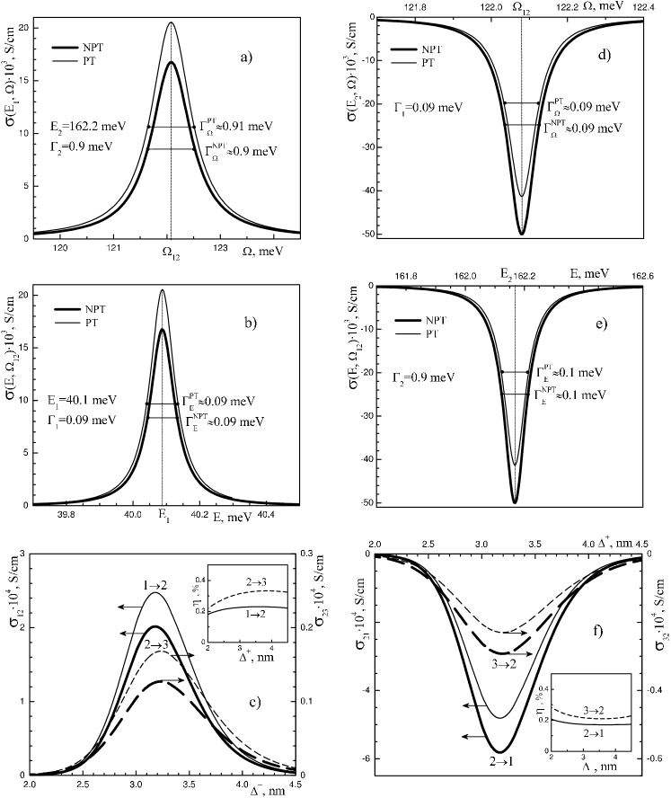
Figure 2: Dependences of maximal magnitudes of positive (a, b, c) and negative (d, e, f) conductivities $\sigma$ on electromagnetic field energy $\Omega=\hbar\omega$ (a, d) and electron energy $E$ (b, e) in two-barrier RTS at $\Delta^{+}=\Delta^{-}$=3 nm. Dependences of maximal magnitudes of positive and negative conductivities on the relationship between the both barrier widths (c, f) at $\Delta^{+}+\Delta^{-}$= 6 nm obtained within the non-perturbation theory (bold solid and dashed curves) and perturbation theory (thin solid and dashed curves).

4 Conclusions

1. The non-perturbation theory of active dynamic conductivity for the open two-barrier RTS, preserving the terms linear over the electromagnetic field in an electron wave function, is proposed for the first time.

2. It is shown that the properties of positive and negative conductivities of two-barrier RTS, shown earlier within the linear approximation over the field perturbation theory, in the so-called weak signal approximation are not only qualitatively similar but quantitatively correlate to the results of a more exact non-perturbation theory proposed.

3. The developed non-perturbation theory of dynamic conductivity for the two-barrier nano-structure can be used for the multi-shell RTS and generalized for the physically and technically important case of electron currents interacting with strong electromagnetic fields in quantum cascade lasers and detectors.

Непертурбацiйна теорiя електронної динамiчної провiдностi двобар’єрної резонансно-тунельної наноструктури М.В.Ткач, Ю.О.Сетi, О.М.Войцехiвська Чернiвецький нацiональний унiверситет iм. Ю.Федьковича, вул. Коцюбинського, 2, 58012 Чернiвцi, Україна

References

• [1] Faist J., Capasso F., Sivco D.L., Sirtori C., Hutchinson A.L., Cho A.Y., Science, 1994, 264, 553; doi:10.1126/science.264.5158.553.
• [2] Faist J., Capasso F., Sirtori C., Appl. Phys. Lett., 1995, 66, 538; doi:10.1063/1.114005.
• [3] Gmachl C., Capasso F., Sivco D.L., Cho A.Y., Rep. Prog. Phys., 2001, 64, 1533; doi:10.1088/0034-4885/64/11/204.
• [4] Golant E.I., Pashkovskii A.B., Phys. Tehn. Poluprovodnikov, 1994, 28, 954 (in Russian).
• [5] Belyaeva I.V., Golant E.I., Pashkovskii A.B., Semiconductors, 1997, 31, 103; doi:10.1134/1.1187090.
• [6] Pashkovskii A.B., JETP Lett., 2005, 82, 210; doi:10.1134/1.2121816.
• [7] Elesin V.F., J. Exp. Theor. Phys., 1997, 85, 264; doi:10.1134/1.558273.
• [8] Elesin V.F., J. Exp. Theor. Phys., 2002, 94, 794; doi:10.1134/1.1477905.
• [9] Elesin V.F., J. Exp. Theor. Phys., 2005, 100, 116; doi:10.1134/1.1866204.
• [10] Tkach M.V., Makhanets O.M., Seti Ju.O., Dovganiuk M.M., Voitsekhivska O.M., J. Phys. Stud., 2010, 14, 3703 (in Ukrainian).
• [11] Diez E., Sanchez A., Dominguez-Adame F., Phys. Lett. A, 1996, 215, 103; doi:10.1016/0375-9601(96)00202-2.
• [12] Rapedius K., Korsch H.J., J. Phys. A: Math. Theor., 2009, 42, 425301; doi:10.1088/1751-8113/42/42/425301.
• [13] Kraynov V.P., Ishkhanyan H.A., Phys. Scr., 2010, 140, 014052; doi:10.1088/0031-8949/2010/T140/014052.
• [14] Tkach N.V., Seti Yu.A., Low Temp. Phys., 2009, 35, 556; doi:10.1063/1.3170931.
• [15] Tkach M.V., Seti Yu.O., Ukr. J. Phys., 2010, 55, 798.
• [16] Tkach M.V., Makhanets O.M., Seti Ju.O., Dovganiuk M.M., Voitsekhivska O.M., Acta Phys. Pol. A, 2010, 117, 965.
• [17] Tkach N.V., Seti Ju.A., Semiconductors, 2011, 45, 376; doi:10.1134/S1063782611030195.
• [18] Seti Ju., Tkach M., Voitsekhivska O., Condens. Matter Phys., 2011, 14, 13701; doi:10.5488/CMP.14.13701.
• [19] Tkach M.V., Seti Ju.O., Matijek V.O., Voitsekhivska O.M., Condens. Matter Phys., 2011, 14, 23704; doi:10.5488/CMP.14.23704.
• [20] Golant E.I., Pashkovskii A.B., Semiconductors, 2000, 34, 327; doi:10.1134/1.1187981.
• [21] Jeffreys H., Swirles B., Methods of Mathematical Physics (3rd ed.). Cambridge University Press, 2000.
• [22] Landau L.D., Lifshitz E.M., Quantum Mechanics: Non-Relativistic Theory. Pergamon Press, 1977.
• [23] Tkach N.V., Seti Ju.A., Phys. Solid State, 2011, 53, 590; doi:10.1134/S1063783411030322.
• [24] Landau L.D., Lifshitz E.M., Pitaevskii L.P., Electrodynamics of Continuous Media (2nd ed.). Butterworth-Heinemann, 1984.
\ukrainianpart