Joining Forces of Bayesian and Frequentist Methodology: A Study for Inference in the Presence of Non-Identifiability

Abstract

identifiability, profile likelihood, Bayesian Markov chain Monte Carlo sampling, posterior propriety, propagation of uncertainty, prediction uncertainty Increasingly complex applications involve large datasets in combination with non-linear and high dimensional mathematical models. In this context, statistical inference is a challenging issue that calls for pragmatic approaches that take advantage of both Bayesian and frequentist methods. The elegance of Bayesian methodology is founded in the propagation of information content provided by experimental data and prior assumptions to the posterior probability distribution of model predictions. However, for complex applications experimental data and prior assumptions potentially constrain the posterior probability distribution insufficiently. In these situations Bayesian Markov chain Monte Carlo sampling can be infeasible. From a frequentist point of view insufficient experimental data and prior assumptions can be interpreted as non-identifiability. The profile likelihood approach offers to detect and to resolve non-identifiability by experimental design iteratively. Therefore, it allows one to better constrain the posterior probability distribution until Markov chain Monte Carlo sampling can be used securely. Using an application from cell biology we compare both methods and show that a successive application of both methods facilitates a realistic assessment of uncertainty in model predictions.

1 Introduction

In many scientific situations mathematical models are used to predict properties of a system under study using explicitly formulated assumptions and hypotheses. This is especially important for complex applications that do not allow for an intuitive understanding of the processes involved. Applications range from analyses in particle physics [1] or in climate research [2, 3] to quantifying dynamical processes in cell biology [4]. Often, these mathematical models contain parameters that are unknown or known only with large uncertainty. For example in bio-chemical models that are utilised in cell biology, parameters such as reaction rate constants, amount of molecular compounds, detection sensitivities or measurement backgrounds are often unknown. Before a model can be used for prediction reliably, the unknown parameters have to be estimated by comparing model output to experimental data.

For a realistic assessment of the accuracy of model predictions, it is important that uncertainties in the experimental data and in prior assumptions are propagated correctly via the parameters to the desired predictions. Bayesian Markov chain Monte Carlo (MCMC) sampling facilitates this propagation of uncertainties by sampling from the posterior probability distribution [5]. However, if experimental data is limited and the mathematical models are non-linear and contain many unknown parameters the posterior probability distribution can be insufficiently constrained. For such insufficiently constrained posterior the probability mass can be distributed widely in a high dimensional parameter space. Consequently, MCMC sampling can quickly become infeasible.

Alternatively, one can resort to frequentist methods in this situation. Here, insufficient experimental data and prior assumptions can be interpreted as non-identifiability of the model parameters [6]. We applied a generic approach that uses the profile likelihood to detect both structural and practical non-identifiability [7]. Furthermore, this approach allows one to design new experiments that resolve non-identifiability. Therefore, it is beneficial to further constrain the posterior probability distribution until MCMC sampling can be applied reliably and efficiently.

We compared the results of both MCMC sampling and profile likelihood methods. In the absence of non-identifiability the results of both methods are in good agreement. However, in the presence of non-identifiability their results can be substantially different. Our results imply that MCMC sampling in the presence of non-identifiability can be misleading. Therefore, we suggest a successive application of both methods that ensures a realistic assessment of uncertainty in model predictions.

1.1 Frequentist methods

Maximum likelihood estimation of model parameters is a theoretically well developed area [8]. Based on an assumption on the distribution of the measurement noise, the likelihood function $L(y|\theta)$ of the data $y$ given the parameters $\theta$ describes the agreement of model output and experimental data. In case of normally distributed measurement noise $\epsilon\sim\mathrm{N}(0,\sigma^{2})$ the likelihood reads as

$$L(y|\theta)=\prod_{k=1}^{m}\prod_{l=1}^{d_{k}}\,\frac{1}{\sqrt{2\pi\sigma_{kl}^{2}}}\,\exp\left(-\frac{1}{2}\left(\frac{y_{kl}-y_{k}(t_{l},\theta)}{\sigma_{kl}}\right)^{2}\right)$$ (1)

where $m$ model outputs $y_{k}(t_{l},\theta)$ and $d_{k}$ data instances for each model output such as time points $t_{l}$ can be considered. The maximum of $L(y|\theta)$, i.e. the best fit of the model to the data, provides a point estimate $\hat{\theta}$ of the parameters. This maximum likelihood estimate (MLE) can be calculated for non-linear models by numerical optimisation methods, see e.g. the trust region algorithm in [9] and for a general introduction in [10, 11]. The uncertainty of the estimate $\hat{\theta}$ is buried in the shape of the likelihood function. Figure 1 shows an illustration of the likelihood for three typical cases.

If the amount of model quantities that can be accessed by experiments is limited, a subset of parameters can be structurally non-identifiable. This indicates that the parametrisation of the model is such that two or more parameters can compensate their effects and yield exactly the same model outputs $y_{k}(t_{l},\theta)$. This in turn results in a constant likelihood value on a sub-manifold, see figure 1A. Consequently, the MLE for the parameters cannot be determined uniquely. The parameter relations that cause the structural non-identifiability are akin to gauge invariances in physical theories. However, for complex models it can be difficult to detect structural non-identifiability. For example, if models can only be evaluated by numerical simulation, such as in the case of detector models used in particle physics [12] or dynamical models that are used in cell biology [4], structural non-identifiability cannot be detected directly. In the latter case, methods for a priori structural non-identifiability analysis exist that analyse the structure of the ordinary differential equations (ODE) without having an analytical solution. A comparison of these methods can be found in [13]. However, a priori methods are often limited to linear ODE systems or are impractical for models containing many parameters [14]. Arguably one of the the most practical a priori methods that has also been proved to work for larger models applies a probabilistic algorithm [15, 16].

In addition to structural non-identifiability, model parameter can be practically non-identifiable [7]. This type of non-identifiability arises if the amount and quality of experimental data is limited. It cannot be detected by a priori methods. However, practical non-identifiability is of equal importance. A generic approach that allows one to detect both structural and practical non-identifiability at the same time uses the concept of the profile likelihood [7, 17]. The profile likelihood $PL$ can be calculated for each parameter $\theta_{i}$ individually by

$$PL(y|\theta_{i})=\max_{\theta_{j\not=i}}[L(y|\theta)].$$ (2)

The equation indicates that for each value of $\theta_{i}$ all of the remaining parameters $\theta_{j}$ are re-optimised, see figure 1 for illustration. The profiles $PL(y|\theta_{i})$ break down the uncertainty contained in the high-dimensional likelihood $L(y|\theta)$ to a footprint in one dimension. It allows for reliable conclusions, about whether a parameter can be inferred from the experimental data. Three typical cases arise and can be detected from the profiles. A flat profile with a constant value indicates structural non-identifiability (c.f. figure 1A). A profile that decreases but tails out to a plateau to one or both sides indicates practical non-identifiability (c.f. figure 1B). A profile that tails out to zero on both sides quickly enough, i.e. at least exponentially fast, indicates structural and practical identifiability (c.f. figure 1C). Experimental design and model reduction strategies based on the profile likelihood allows one to resolve parameter non-identifiabilities iteratively, for an application see in [18].

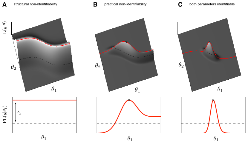
Figure 1: Identifiability analysis using likelihood profiles: The upper panels show as illustration the shape of the likelihood $L(y|\theta)$ in two dimensions for three typical cases. The traces of the profiles in parameter space are indicated as red lines. The lower panels shows the respective profile likelihood $PL(y|\theta_{1})$ for the dimension of parameter $\theta_{1}$ as red lines. In all panels the asterisks denote the MLE in cases where a unique solution exists and the dashed lines denote the threshold $\Delta_{\alpha}$ that yields a likelihood based confidence region [19, 10]. Three typical cases can arise: (A) A flat profile indicates structural non-identifiability. In this case, no unique solution for MLE exist. (B) A profile that decreases but tails out to a plateau to one or both sides indicates practical non-identifiability. (C) A profile that tails out to zero on both sides quickly enough, i.e. at least exponentially fast, indicates structural and practical identifiability. The confidence interval of $\theta_{1}$, for (A) is infinite, for (B) has only a lower bound, for (C) has a finite range.

Furthermore, the profile likelihood allows one to assess likelihood based confidence intervals [20, 21, 22]. A confidence interval $[\sigma_{i}^{-},\,\sigma_{i}^{+}]$ to a confidence level $\alpha=0.95$ signifies that the true value of the parameter $\theta^{*}_{i}$ is expected to be inside the interval with 95% probability. Using a threshold $\Delta_{\alpha}=\mathrm{Q}(\chi^{2}_{df},\,\alpha)$ which is the $\alpha$ quantile of the $\chi^{2}$–distribution with $df$ degrees of freedom [10], confidence intervals can be determined from the profiles by $\{\theta_{i}\,\,|-2\cdot\log(PL(y|\theta_{i})/L(y|\hat{\theta}))<\Delta_{\alpha}\}$.

1.2 Bayesian methods

By applying Bayes’ theorem the likelihood function (1) is extended by the prior probability density function (PDF) of the parameters $P(\theta)$ and normalised by a factor $c$ yielding the posterior PDF of the parameters

$$P(\theta|y)=c\cdot L(y|\theta)\cdot P(\theta).$$ (3)

In analogy to the MLE, the maximum a posteriori (MAP) estimate is defined by maximising $P(\theta|y)$. The only decisive difference to frequentist methodology is the choice of the prior $P(\theta)$. The direct computation of the normalisation factor $c$ is not feasible for a high dimensional parameter space. However, extensive Markov chain Monte Carlo (MCMC) sampling offers a way to evaluate $P(\theta|y)$ despite unknown $c$. This intriguing feature opens the prospect of considering the full high dimensional posterior PDF for statistical inference. Most prominently, the Metropolis-Hastings algorithm [23, 24] defines a Markov process where transitions $\theta\rightarrow\theta^{\prime}$ are generated using a proposal function $q(\theta|\theta^{\prime})$ that eventually produces a series of samples of the posterior PDF $P(\theta|y)$. The transitions are accepted with probability

$$\alpha(\theta,\theta^{\prime})=\min[1,\left(L(y|\theta^{\prime})/L(y|\theta)\right)\cdot\left(q(\theta|\theta^{\prime})/q(\theta^{\prime}|\theta)\right)].$$ (4)

For efficiency of the sampling the choice of the proposal function $q(\theta|\theta^{\prime})$ is important. Often, proposals drawn from a multivariate normal distribution are convenient. One of the most simple implementations uses $q(\theta|\theta^{\prime})\sim\mathrm{N}(0,s\cdot\mathbb{I})$ where $s\cdot\mathbb{I}$ is a scaled identity matrix (SIM). Too small a choice of $s$ in relation to the actual shape of the posterior PDF will cause the process to converge slowly and to produce correlated samples. Too large a choice of $s$ will lead to rejection of too many proposals $\theta^{\prime}$ yielding a slow sampling. Assuming that the posterior PDF is a multivariate normal distribution the optimal acceptance rate of proposals is $\approx 0.23$ [25]. Nevertheless, in the light of complex and non-linear models with possibly limited amount and accuracy of experimental data, this assumption is problematic because the shape of the posterior PDF can be far from the PDF of a normal distribution. For a high dimensional parameter space computational efficiency also becomes an important issue. In these cases, the Markov chain may have to move along complex structures [19, figure 8.2.2]. To increase efficiency more sophisticated methods take into account the natural geometry of the posterior PDF, e.g. the manifold Metropolis adjusted Langevin algorithm (MMALA) takes into account the local gradient and curvature information [26].

Before applying an MCMC sampling method, the prior PDF of the parameters needs to be specified. Given that empirical evidence exists about the distribution of a parameter, such as a previous measurements or estimation, $P(\theta)$ should incorporate this prior knowledge accordingly [27]. If no empirical evidence about the parameter value is available, the prior should be chosen as uninformative [19]. This requires a flat metric in parameter space, i.e. that does not artificially favour certain parameter values. Depending on the parametrisation of the model it can in practice be difficult to obtain a flat metric and hence to specify an uninformative prior [27].

The most crucial problem that MCMC sampling faces is to ensure that the samples obtained realistically represent the actual posterior PDF. One instance where the convergence of the Markov chain fails is if the posterior PDF is not proper [28]. Posterior PDF’s are called proper if they are integrable [19]. This means that it has to tail out to zero sufficiently fast over the appreciable range of the parameters such that its integral can be normalised to one. Non-identifiable parameters cause the posterior PDF to be non-proper [28]. This indicates that neither the prior assumptions nor the likelihood that represents the experimental data constrain the posterior PDF sufficiently. A practical consequence is that the Markov chain cannot converge and hence gives inaccurate results [29]. For convergence it is required that the Markov chain is positive recurrent which is not given in the case of non-identifiability [30]. The user must ensure parameter identifiability before an MCMC technique can be used securely. If models contain many unknown parameters and the posterior PDF is not sufficiently constrained the convergence of the Markov chain can be impractically slow even for a proper posterior PDF.

2 Results

For reliable inference in the presence of non-identifiability, we propose a joint approach that takes advantage of both profiling and MCMC sampling methods. The profile likelihood is suitable to detect parameter non-identifiability [7]. Furthermore, it allows for experimental design that helps to resolve parameter non-identifiability [18]. This ensures that the posterior PDF is proper and well constrained. Subsequently, efficient MCMC sampling [26] can be used reliably to generate samples of the posterior PDF. Finally, the uncertainty in model predictions can be assessed realistically. The workflow of this joint approach is displayed in figure 2A.

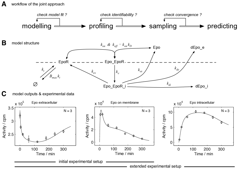
Figure 2: (A) Workflow of the joint approach that combines profile likelihood and MCMC sampling methods: The first step is setting up an appropriate mathematical model (B) that contains the available prior knowledge and explains the experimental data sufficiently well (C). The profile likelihood approach allows one to detect and to resolve non-identifiability by experimental design. Therefore, it helps to ensure that the posterior PDF is proper and sufficiently well constrained. Subsequently, MCMC sampling can be applied securely. Finally, the uncertainty in model predictions can be assessed realistically using the obtained samples. (B) The figure shows the structure of the ODE model describing Epo and EpoR interactions. The dashed line indicates the cell membrane, the part above is the outside, the part below is the inside of the cell. (C) The agreement of experimental data and model output for MAP parameter values for both experimental setups is displayed. The extended setup was derived by experimental design considerations, see in [18].

Both profiling and MCMC sampling methods separately are used for inference in various fields, e.g. in particle physics [31, 1] or in climate research [3, 2]. Here, we present results of using the joint approach that takes advantage of both methods for an application from cell biology [32]. An ordinary differential equation (ODE) model was used to describe the concentration dynamics of six molecular compounds involved in the interplay of the hormone erythropoietin (Epo) and its corresponding membrane receptor (EpoR), see figure 2B. Epo is an important factor in the differentiation of blood cells. The dynamics of the molecular compounds are formulated as

$$\mathrm{d}\vec{x}(t,\theta)/\mathrm{d}t=\vec{f}(\vec{x}(t,\theta),\theta)$$ (5)

and a mapping of the dynamics to experimentally accessible quantities by the model output function

$$\vec{y}(t,\theta)=\vec{g}(\vec{x}(t,\theta),\theta)$$ (6)

that enters the likelihood function (1) was used. The model comprises six ODEs and ten unknown parameters including one nuisance parameter, for details about the model equations see the supplementary notes. All parameters are positive by definition, hence the logarithmic space yields a flat metric [19]. Since no empirical evidence about the values of the nine parameters of interest was available the prior was chosen uninformative.

Radioactively labeled Epo facilitated the measurement of Epo concentration in the extracellular medium and of Epo bound to the cell membrane, see supplementary table 1. The MAP estimates of the model parameters were obtained by numerical optimisation, see supplementary table 2. The agreement of model outputs and experimental data for this initial experimental setup is shown in figure 2C. In accordance with the experimental data the model describes the binding of Epo to the Epo receptor on the membrane, internalisation and recycling of the Epo-EpoR complex. As first step of the proposed joint approach the posterior PDF was screened for non-identifiability using the profiling method.

2.1 Identifiability analysis using posterior profiles

The profile likelihood approach for identifiability analysis [7] can be translated to a profile posterior approach. In analogy to equation (2) profiling can be applied to the unnormalised posterior PDF by defining the profile posterior

$$PP(\theta_{i}|y)=\max_{\theta_{j\not=i}}[P(\theta|y)],$$ (7)

c.f. figure 1. Technical details on the implementation of the methods are given in the supplementary notes. For the initial experimental setup, the profiles of the posterior PDF reveal four structurally non-identifiable, two practically non-identifiable and three identifiable parameters. One of each case is displayed as red lines in figure 3A, the remaining profiles are shown in supplementary figure 1.

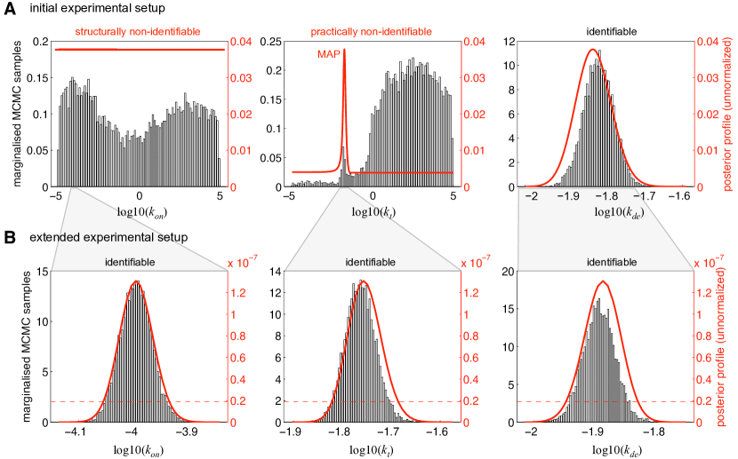
Figure 3: Comparison of profiling and sampling results: (A) For the initial experimental setup the posterior profiles indicated by red lines reveal that parameter $k_{on}$ is structurally non-identifiable, parameter $k_{t}$ is practically non-identifiable and parameter $k_{de}$ is identifiable. The histograms display the marginalised MCMC samples obtained by the MMALA algorithm. For the identifiable parameter $k_{de}$ both results of profiling and sampling agree quite well. Also for the structurally non-identifiable parameter $k_{on}$ the agreement is acceptable. For the practically non-identifiable parameter $k_{t}$ the results are substantially different. The profile shows that the MAP point is located at $\log_{10}(k_{t})\approx-1.8$. However, the lion’s share of the marginalised MCMC samples propose $\log_{10}(k_{t})$ to be $>0$. (B) Taking into account more experimental data the posterior profiles for the extended experimental setup indicate that all parameters are now identifiable. The results of MCMC sampling and profiling are in good agreement. Interestingly, the MCMC samples for parameter $k_{t}$ for the extended setup are localised close to the MAP point of the initial setup, note the different scales on the x-axis for (A) and (B). The dashed red lines indicates the threshold $\Delta_{\alpha}$ that can be used to assess likelihood based confidence intervals.

2.2 Markov chain Monte Carlo sampling

The results of the posterior profiling approach indicates that the posterior PDF for the initial experimental setup is not proper, i.e. the posterior PDF cannot be normalised to one and is therefore not a valid PDF. In this situation an MCMC sampling cannot converge and hence gives inaccurate results [29]. In order to allow for a comparison between profiling and MCMC sampling, the prior PDF was restricted artificially to a uniform distribution with support from $10^{-5}$ to $10^{+5}$. The resulting posterior PDF is now proper and the Markov chain can in principle converge. It is important to note that the results of MCMC sampling can potentially be biased due to the artificial specification of this prior PDF. The new posterior PDF, though proper, still exhibits a complicated structure. The probability mass is distributed widely in the ten dimensional parameter space, see the posterior profiles in figure 3A. In this situation, the SIM sampling algorithm, that uses a scale identity matrix for generating proposals, was too inefficient and did not yield reasonable results within an acceptable time, see supplementary figures 1–3. To improve efficiency the MMALA algorithm that takes into account the local geometry of $P(\theta|y)$ was used [26]. Figure 3A shows the histograms of marginalised MCMC samples. The remaining results are displayed in supplementary figures 4–6. For the identifiable parameter $k_{de}$ and for the structural non-identifiable parameter $k_{on}$ the results of the MCMC sampling are in good agreement with the results of the profiling. For the practically non-identifiable parameter $k_{t}$ the results are substantially different. The profile shows that the MAP point is located at $\log_{10}(k_{t})\approx-1.8$. However, the lion’s share of the marginalised MCMC samples propose $\log_{10}(k_{t})$ to be $>0$. In this region the posterior profile reveals a plateau.

2.3 Taking into account additional experimental data.

Both the results of posterior profiling and MCMC sampling indicate substantial uncertainty in the parameter estimates for the initial experimental setup. Based on the results of the profiling approach additional experiments were suggested, see in [18] for details. The target of the experimental design was to resolve non-identifiabilities. The additional experimental data were included in the estimation procedure, yielding an extended experimental setup, see figure 2C. Figure 3B shows the recomputed posterior profiles. They indicate, by tailing out to zero, that the identifiability problems were resolved for all parameters. The remaining profiles are shown in supplementary figure 7.

As a consequence the posterior PDF is now proper without artificial assumptions on the prior PDF. In this situation, the SIM sampling algorithm was still too inefficient and did not yield reasonable results within an acceptable time, see supplementary figures 7–9. To improve efficiency the MMALA algorithm that takes into account the local geometry of $P(\theta|y)$ was used again [26]. Figure 3B shows the histograms of marginalised MCMC samples. The results for the remaining parameters are shown in supplementary figures 10–12. For all parameters the results of the MCMC sampling and posterior profiling are now in good agreement. The MCMC samples for parameter $k_{t}$ that showed substantial difference between profiles and MCMC samples for the initial setup are now in good agreement as well. Interestingly, the MCMC samples for parameter $k_{t}$ for the extended setup are localised close to the MAP point of the initial setup. This suggests that the large probability mass of MCMC samples for values of $\log_{10}(k_{t})>0$ obtained for the initial setup was misleading.

MCMC sampling results are now reliable and allow one to consider the full high dimensional posterior PDF for inference, see e.g. the non-linear correlation between parameter $k_{di}$ and $k_{de}$ shown in supplementary figure 13. Using the generated MCMC samples, the parameter uncertainties contained in the posterior PDF can be propagated accurately to the prediction of the dynamics of molecular compounds that are not accessible by experiments directly, see figure 4.

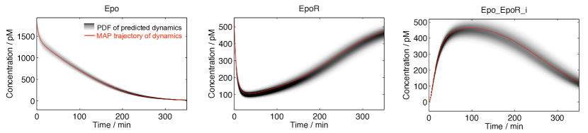
Figure 4: Propagation of parameter uncertainties to model predictions: The posterior samples that were acquired by MCMC sampling for the extended setup, see figure 3B, can now be used to assess prediction uncertainties accurately. The figure shows the predicted dynamics of three molecular components that could not be measured directly. The red line shows the prediction that corresponds to the MAP estimate of the parameters. The grey scale displays the posterior PDF of the prediction.

3 Summary

We introduced a joint approach that combines frequentist profiling and efficient Bayesian MCMC sampling methods. The proposed approach uses the analysis of posterior profiles that helps to determine the identifiability of the model parameters. Non-identifiability results in a posterior distribution that is not proper, i.e. that cannot be normalised to one. However, a proper posterior distribution is required for convergence of the MCMC sampling. The results of the posterior profiling can be used for experimental design that helps resolve non-identifiabilities iteratively. Consequently, this ensures that the posterior distribution is proper. Having ensured identifiability of the parameters, the MCMC sampling results are reliable and can be used to propagate the uncertainty of parameter estimates to model predictions. Using an application from cell biology we showed that this approach enables one to obtain accurate results.

We compared the results of posterior profiling and marginalising over the MCMC samples for two stages of experimental setup: an initial setup that contains non-identifiabilities and an extended setup where all parameters are identifiable. A uniform prior distribution ensured that the posterior is proper despite non-identifiability for the initial setup. For the extended setup the results of posterior profiling and marginalising over the MCMC samples are in good agreement. For the initial setup substantial difference between profiles and MCMC samples are observed. Interestingly, the profiles for the initial setup reflect the posterior distribution for the extended setup much better than the MCMC samples of the initial setup. This indicates that MCMC sampling results in the presence of non-identifiability can be inaccurate despite a proper posterior distribution.