An Exercise in Invariant-based Programming with Interactive and Automatic Theorem Prover Support

Abstract

Invariant-Based Programming (IBP) is a diagram-based correct-by-construction programming methodology in which the program is structured around the invariants, which are additionally formulated before the actual code. Socos is a program construction and verification environment built specifically to support IBP. The front-end to Socos is a graphical diagram editor, allowing the programmer to construct invariant-based programs and check their correctness. The back-end component of Socos, the program checker, computes the verification conditions of the program and tries to prove them automatically. It uses the theorem prover PVS and the SMT solver Yices to discharge as many of the verification conditions as possible without user interaction. In this paper, we first describe the Socos environment from a user and systems level perspective; we then exemplify the IBP workflow by building a verified implementation of heapsort in Socos. The case study highlights the role of both automatic and interactive theorem proving in three sequential stages of the IBP workflow: developing the background theory, formulating the program specification and invariants, and proving the correctness of the final implementation.

1 Introduction

Invariant-based programming (IBP) is a method for formal verification of imperative programs [4]. It is a correct-by-construction method: the correctness proofs are developed hand-in-hand with the program. In IBP the internal loop invariants of the program are also written before the code. After the invariant structure has been established, the code is added in small increments, and each extension is verified to preserve the invariants. Letting the correctness arguments determine the structure of the code, rather than vice versa, makes the verification task significantly less difficult compared to verification a posteriori. IBP has been successfully applied as a pedagogical device in teaching introductory formal methods [5].

The correctness of even small programs depends on a large number of verification conditions to be proved. We are building a programming environment called Socos, which applies state-of-the-art automatic theorem proving tools and satisfiability modulo theories (SMT) solvers to discharge as many of the lemmas as possible without user intervention. The front-end to the system is a graphical diagram editor, supporting both constructing the program and checking its correctness. This front-end is implemented as a plug-in for Eclipse [2]. The back-end program checker derives the verification conditions from the program source, and interfaces with the theorem prover PVS [19] to automatically discharge as many of the conditions as possible. Socos allows the full higher-order logic of PVS in specifications and invariants. Hence, all conditions could not be proved automatically. Conditions that were not automatically discharged can be proved interactively in the PVS proof assistant. Alternatively, proof automation can often be improved by introducing abstractions which are more suitable for automatic reasoning in the domain of discourse. Such abstractions can be added to the verification process through background theories, and domain-specific proof strategies based on background theories can significantly improve proof automation.

This paper presents the workflow of Socos-supported IBP in the context of a case study. We first describe IBP in general, followed by a overview of Socos from both a user and a systems level perspective. Next, we build a set of PVS background theories for dynamic arrays, sortedness and permutations. Finally, based on these theories we build a verified implementation of heapsort. The case study focuses on the interplay between programming and proving, and describes how the complete workflow from specification to verified implementation is supported by Socos. Although the code itself is small, verification of heapsort involves several nontrivial invariants and proofs. The specification involves the notions of sortedness, permutations, and heaps. We extend the background theories by proving additional lemmas in PVS to improve automation while maintaining soundness with respect to the base definitions. The case study also shows how Socos can identify bugs related to corner cases, which are otherwise easily missed during testing.

Related work.

IBP builds on early work by Back [3], Reynolds [21], van Emden [15]. A comprehensive overview of the method is given in [4]. A description of the semantics and proof theory of IBP can be found in [8]. There exists a large number of verification tools based on VC generation and theorem proving. PVS verification of Java programs is supported by Loop [11] and the Why/Krakatoa tool suite [17]. Several program verifiers are based on SMT solvers. Boogie [9] is an automatic verifier of BoogiePL, a language intended as a backend for encoding verification semantics of object oriented languages. Spec#, an extension to C#, is based on Boogie [10]. Back and Myreen have developed an automatic checker for invariant diagrams [7] based on the Simplify validity checker [13]. Together with the second author they later developed the checker into a prototype of the Socos environment [6].

Overview of paper.

The remainder of the paper is as follows. Section 2 introduces the notion of invariant diagrams and their correctness. Section 3 describes the Socos environment from the user perspective. Section 4 gives a systems-level overview of Socos, focusing on the interface to the underlying components (PVS and Yices). In Section 5 we develop a background theory for dynamic arrays, sortedness and permutations. Section 6 develops the case study, a verified implementation of heapsort. Section 7 concludes the paper with a summary and some observations.

2 Invariant diagrams

The basic building blocks of invariant-based programs are situations and transitions. Situations are predicates over the state space of the program, whereas transitions are program statements. Invariant diagrams are directed, nested graphs where the nodes correspond to situations and the edges correspond to transitions. The operational interpretation of an invariant diagram is that of a state chart: control flows from situation to situation by (nondeterministically) following enabled transitions. A transition is enabled if its guard holds in the current state. Figure 1a shows an IBP implementation of the selection sort algorithm. Situations are drawn as rectangles with rounded corners, transitions as arrows connecting the rectangles. The predicate (invariant) of a situation is written in the top left corner of the situation. Statements—sequential composition of guards and assignments—are written adjacent to the transition arrows. The program consists of an inner and an outer loop. Each iteration of the outer loop extends the sorted portion with one element by finding (in the inner loop) the minimal element in the unsorted portion (at index $m$) and then exchanging it with the first element in the unsorted portion (at index $k$). The invariant of the inner loop is stronger than that of the outer loop. Nesting the inner loop situation inside the outer loop situation indicates that the invariant of the outer loop should be inherited.

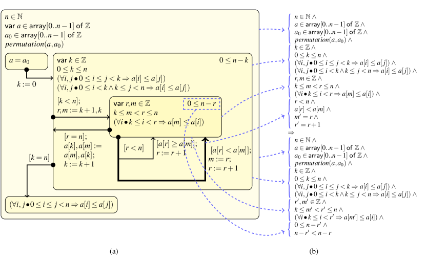
Figure 1: (a) invariant diagram for selection sort; (b) consistency and termination conditions for the bolded loop transition

An invariant-based program is correct if execution, when started from any one situation, terminates in a final situation. A final situation is a situation with no outgoing transitions. Final situations correspond to the postcondition(s) of the program. An invariant diagram can be interpreted as a total correctness theorem, where each transition corresponds to a consistency lemma, each intermediate (non-final) situation corresponds to a liveness lemma, and each loop corresponds to a termination lemma. A transition is consistent if the source situation, the guard and the assignments imply the target situation. An intermediate situation is live if at least one outgoing transition is always enabled. A loop is terminating if each cycle strictly decreases a termination function, i.e., a function from the program states to a well-founded set. The termination function is written together with its lower bound in the upper right hand corner of the recurring situation. A diagram is correct iff all transitions are consistent, all intermediate situations are live, and all loops are terminating.

The programmer first defines the situation structure, and then adds and checks the transitions one by one. The lemma to be checked for a transition can be read directly from the diagram. Figure 1b shows the condition for the loop transition in the example. The antecedent contains the source situation predicate, the guard of the transition, and the equalities introduced by the assignments to variables $m$ and $r$. The consequent contains the same situation predicates over the updated values $m^{\prime}$ and $r^{\prime}$, and additionally a constraint that the termination function of the inner loop ($n-r$) remains bounded from below (by $0$) while strictly decreasing.

3 Invariant-based programming in the Socos environment

Socos supports construction and static checking of invariant-based programs. The top level document, called the verification context, defines global constants, associated PVS background theories, and a default proof strategy. Nested within the verification context is a collection of (mutually recursive) procedures. Each procedure is specified by a precondition and one or more postconditions, and implemented by an invariant diagram. Visually, pre- and postconditions are distinguishable from intermediate situations by the outline: preconditions are drawn with a thick outline, whereas postconditions are drawn with a double outline. If the precondition is omitted, it defaults to true and the initial transition is drawn from the procedure outline. The transition language supports sequential composition of assumptions, assertions, assignments, and procedure calls. All expressions, including guard expressions and the right hand side of assignments, are written in the PVS syntax.

The programmer edits the verification context and its contained diagrams in a graphical environment (Figure 2). By the click of a button, Socos generates the verification conditions from the diagram, attempts to discharge as many as possible automatically, and then reports the unproved conditions to the programmer.

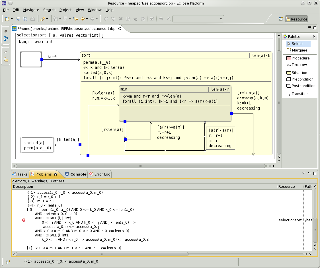
Figure 2: The Socos programming environment

Figure 2 shows a session in which the program in Figure 1, implemented as a Socos procedure, is being checked. In this case, the program contains an error: the second loop transition has the increment $\mathtt{r:=r+1}$ and assignment $\mathtt{m:=r}$ in the wrong order. Consequently, the loop invariant is not preserved by the transition. Socos pinpoints the inconsistency by highlighting the loop transition, and the unproved (false) condition associated with the transition becomes visible in the “Problems view”.

Invariant diagrams are built and checked incrementally, i.e., transition by transition. Hence, all transitions may not be in place when the program is checked. Consistency is always checked for all transitions that have been added so far to the diagram. Liveness and termination checking can be postponed. For instance, omitting the termination function disables generation of termination conditions, and instead Socos prints a warning that the program may not be terminating.

4 System overview

Figure 3 shows the components of Socos and their interdependencies. In this section, we briefly describe these components.

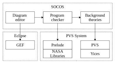
Figure 3: Software architecture

4.1 Diagram editor

The diagram editor is implemented as an extension to Eclipse [2], an extensible platform for tool integration. Eclipse extensions, called plug-ins, implement a set of standardized extension points provided by Eclipse to implement the functionality of the plug-in. The user interface of Eclipse follows a workspace metaphor, in which the user manages a set of resources through views and editors. A view is a UI component displaying a resource; editors allow both viewing and updating a resource. The Socos plug-in adds an invariant diagram editor built on top of the Graphical Editing Framework (GEF) provided by Eclipse. The editor’s associated tool palette, shown in the right hand side of Figure 2, contains tools for code editing, situation placement, and transition routing. Clicking the “check button” sends the diagram to the program checker, which can be called either locally (over Unix pipes) or remotely (over http).

4.2 Program checker

The program checker generates a PVS translation of the verification conditions for the diagram. The verification conditions are calculated by weakest preconditions, and exported into a PVS theory file containing a lemma for each condition. To each lemma, the program checker also associates a proof script which is run through the PVS proof checker, and the final proof state (proved or failed) of each condition is collected. Any PVS strategy can be used to attempt to discharge the conditions; the default strategy invokes Yices. We give here only a brief overview of the underlying proof tools and the translation; the verification semantics is described in detail in [16].

PVS and Yices.

PVS is a free, open source theorem proving system based on simply-typed higher-order logic [20]. It provides base types such as bool, nat, int and real, and type constructors to build new types from existing types. Types are related to sets: two types are equal if they denote the same set of values, and subtypes correspond to subsets. For example, $\mathtt{nat}$ is a subtype of $\mathtt{int}$, $\mathtt{int}$ is subtype of $\mathtt{rational}$, and $\mathtt{rational}$ is a subtype of $\mathtt{real}$. Subtypes are introduced by predicate subtyping [22]; the subtype is defined by a predicate on the supertype. Type checking in PVS is undecidable in the general; type correctness conditions (TCCs) generated by the type checker may hence require interactive proof.

PVS proof theory is based on sequent calculus. A proof is a tree where each node is a sequent of the form $\gamma_{1},\dots,\gamma_{n}\vdash\delta_{1},\dots,\delta_{m}$ where $\gamma_{1},\dots,\gamma_{n}$ are the antecedents and $\delta_{1},\dots,\delta_{m}$ are the consequents. PVS proofs are goal-directed: the proof of a proposition $\alpha$ starts with the root sequent $\vdash\alpha$. A command either proves a sequent, or reduces it to subgoals. A proof tree is complete when every leaf is proved. The logic of PVS is embodied in a small set of primitive inference rules. Every command corresponds to a sequence of applications of these rules. Proof strategies are higher-order functions combining basic commands into more powerful commands.

Yices is a free SMT solver which can be used as a decision procedure in PVS [14]. To check the validity of a sequent $\gamma_{1},\dots,\gamma_{n}\vdash\delta_{1},\dots,\delta_{m}$, the command (yices) checks the satisfiability of the formula $\gamma_{1}\land\dots\land\gamma_{n}\land\neg\delta_{1}\land\dots\land\neg\delta_{m}$ using Yices. If the formula is unsatisfiable, the sequent is valid and is thus discharged; otherwise, (yices) does nothing.

Verification condition generation.

The consistency condition for a transition $S_{X,Y}$ from situation $X$ to situation $Y$ is generated based on the rule:

$$\forall\sigma:P_{X}(\sigma)\Rightarrow wp(S_{X,Y})(P_{Y})(\sigma)$$

The variable $\sigma$ ranges over all program states, $P_{X}$ and $P_{Y}$ are the state predicates of the situations $X$ and $Y$, and $wp(S_{X,Y})$ is the weakest precondition predicate transformer for the statement $S_{X,Y}$. Based on this rule, one PVS lemma is generated for each situation, capturing the consistency of all outgoing transitions. Procedure calls are verified consistent based on the pre- and postconditions of the called procedure in the usual way.

A procedure is live if the following conditions both hold: (1) the postcondition is reachable from the precondition; and (2) each statement can proceed from any state it may be reached by (absence of miracles). Condition (1) is checked by analyzing the transition graph. Condition (2) is true for all statements satisfying the “excluded miracle” law: $\forall\sigma:\neg\text{wp}(S)(\emptyset)(\sigma)$. Assignments, procedure calls and guarded choices satisfy this property. Socos also allows assume statements—which may be miraculous—but in this case warns that the program may not be live.

Termination is proved by mapping the situations in a strongly connected component to a well-founded set. Each component must be associated with a function from the program state to $\mathtt{nat}$. Socos generates a verification condition that the value of the termination function strictly decreases by the loop transition. For recursive procedures, the termination function is over the parameter list, and must be shown to decrease by each recursive call.

Proof checking.

Parallel to each generated lemma, the program checker generates a proof script that can be executed by PVS to produce a transcript of the proof run. Socos implements a light-weight interface to the PVS Lisp process, through which the generated proof script is executed and all open (unproved) sequents are collected from the proof transcript. Socos extracts the open sequents on-line as the proof progresses, allowing incremental extension of the proof status report. By applying the primitive inference rules of PVS, the proof script expands the generated correctness lemma into a proof tree where each leaf is of the form

$$\gamma_{1},\dots,\gamma_{n}\vdash\delta$$

where $\gamma_{1},\dots,\gamma_{n}$ are the assumptions from the source situation and transition, and $\delta$ is a single constraint from the target situation. The default proof strategy applied to each such leaf is user-definable. The following PVS strategy, which we will use in the case study, expands all relevant definitions in the sequent, loads the lemmas supplied as parameters into the antecedent, and invokes Yices as an end-game prover:

⬇

(defstep endgame (&optional (lemmas nil))

(let ((introduce-lemmas ‘(then ,@(loop for l in lemmas append ‘((lemma ,l))))))

(then

(skosimp*)

(auto-rewrite-defs :always? t)

(assert)

introduce-lemmas

(yices)

(fail)))

"End-game strategy" "Invoking Yices, supplying lemmas: ~{~a~^, ~}")

Yices either proves the lemma, or the entire strategy fails. Definitions not expanded in the second step appear as uninterpreted constants and the supplied lemmas as axioms to Yices. This allows feeding specific lemmas in cases where automatic reasoning with the definitions is infeasible; the example in Section 5 demonstrates this mechanism.

4.3 Background theories

Socos contexts can directly import PVS background theories containing specifications, definitions and lemmas useful for specifying and verifying invariant diagrams. Good background theories are challenging to develop. For a new domain we spend about half the time developing the background theories, while the other half is spent building and verifying the diagrams. However, the time vested in developing background theories is typically amortized over several programs in the same domain. Background theories can build on existing theories, for instance from the PVS prelude or the comprehensive NASA Langley theory collection [18]. Socos provides a small library of background theories and strategies. It currently consists of just a few basic theories for arrays and vectors, but we plan on extending it based on case studies.

5 Background theories for sorting

This section describes two background theories: vector, introducing a type for dynamic arrays, and sorting, introducing a set of predicates for specifying sortedness and permutations. We will use these theories in program developed in the remainder of the paper.

5.1 Dynamic arrays

PVS dependently typed records provide a convenient way of modeling dynamic (resizable) arrays containing elements of the generic type $\mathtt{T}$:

$\begin{array}[t]{@{}l}\mathtt{vector[T:type+]}:\;\textsf{{theory}}\\ \textsf{{begin}}\\ \quad\begin{array}[t]{l}\mathtt{vector:\textsf{{type+}}=[\#\,len\colon nat,\,elem\colon[below(len)\rightarrow T]\,\#]}\\ \mathtt{index(a:vector)}:\textsf{{type}}=\mathtt{below[len(a)]}\end{array}\end{array}$

The $\mathtt{vector}$ type is a record type with a field $\mathtt{len}$ for the number of elements and field $\mathtt{elem}$ for accessing the contents. The value of the field $\mathtt{elem}$ is a function whose domain depends on value of the field $\mathtt{len}$. The type $\mathtt{below}$ is a dependent type itself, defined as $\mathtt{below(i:nat):\textsf{{type}}=\{s:nat|s<i\}}$ in the PVS prelude. Since PVS is a logic of total functions, $\mathtt{elem(a)}$ may only be applied within its domain; accessing $\mathtt{elem(a)}$ outside its domain will generate unprovable TCCs. The second line introduces the shorthand $\mathtt{index(a)}$ for the domain of $\mathtt{elem(a)}$. Access and update of an element can now be defined as:

$\begin{array}[t]{@{}l}\quad\begin{array}[t]{l}\mathtt{access(a\colon\mathtt{vector},i\colon index(a)):T=elem(a)(i)}\\ \mathtt{update(a\colon\mathtt{vector},i\colon index(a),x:T):vector=}\\ \quad\mathtt{(\#\,len\colon=len(a),elem\colon=elem(a)\,\textsf{{with}}\,[i\colon=x]\,\#)}\end{array}\end{array}$

In the sequel, we will write $\mathtt{a[i]}$ instead of $\mathtt{access(a,i)}$ for brevity. Finally, a predicate that two arrays are element-wise equal on a common subrange will become useful later:

$\begin{array}[t]{@{}l}\quad\begin{array}[t]{l}\mathtt{eql(a\colon\mathtt{vector},b\colon\mathtt{vector},l\colon nat,r\colon nat):bool}=\\ \quad\mathtt{\forall(i:nat):l\leq i\land i<r\land i<len(a)\land i<len(b)\Rightarrow a[i]=b[i]}\\ \end{array}\\ \textsf{{end}}\;\mathtt{vector}\\ \\ \end{array}$

5.2 Sortedness, permutation and swap

We focus in the sequel on sorting arrays of type $\mathtt{vector[int]}$. The postcondition of a sorting program should state that the array (1) is in non-decreasing order, and (2) has preserved all values of the original array. We introduce a predicate $\mathtt{sorted}$ to express property (1) in a new PVS theory:

$\begin{array}[t]{@{}l}\mathtt{sorting}:\;\textsf{{theory}}\\ \textsf{{begin}}\\ \quad\begin{array}[t]{@{}l}\textsf{{importing}}\ \mathtt{vector[int]}\\ \mathtt{a,b,c}:\;\textsf{{var}}\ \mathtt{vector}\\ \mathtt{sorted(a):bool=\forall(i,j:index(a)):i<j\Rightarrow a[i]\leq a[j]}\end{array}\end{array}$

In the sequel we use $\mathtt{sorting}$ as a background theory for our sorting program, extending it with additional definitions as needed. To formalize property (2), we introduce a binary predicate $\mathtt{perm}$, asserting the existence of a bijection over the indexes that makes vectors $\mathtt{a}$ and $\mathtt{b}$ elementwise equal:

$\quad\mathtt{perm(a,b):bool=\begin{array}[t]{@{}l}\mathtt{\mathtt{\exists(f:(bijective?(index(a),index(b)))):}}\\ \quad\mathtt{\forall(i:index(b)):b[i]=a[f(i)]}\end{array}}$

For an automatic prover reasoning in terms of this definition is problematic, since it requires demonstration of a bijection. Quantifiers render Yices incomplete, and the catch-all strategy grind fails to prove even that $\mathtt{perm}$ is reflexive. When verifying algorithms which manipulate pairs of elements it is more fruitful to consider permutation as the smallest equivalence relation that is invariant under the pairwise swap. Proceeding in this direction, we introduce and prove the following properties of $\mathtt{perm}$ in PVS:

$\quad\begin{array}[t]{@{}l}\mathtt{perm\_len:\;\textsf{{lemma}}\ perm(a,b)\Rightarrow len(a)=len(b)}\\ \mathtt{perm\_ref:\;\textsf{{lemma}}\ perm(a,a)}\\ \mathtt{perm\_sym:\;\textsf{{lemma}}\ perm(a,b)\Rightarrow perm(b,a)}\\ \mathtt{perm\_trs:\;\textsf{{lemma}}\ \mathtt{perm(a,b)\land perm(b,c)\Rightarrow perm(a,c)}}\end{array}$

The first lemma states that permutations have equal length, allowing the prover to infer that a valid index in an array is also a valid index in any permutation of the array. The remaining lemmas state that permutation is an equivalence relation. Proving these four lemmas is a straightforward exercise in PVS, involving in each case finding the right instantiation of the bijection $\mathtt{f}$. Next, we introduce a function $\mathtt{swap}$ for exchanging the elements at indexes $\mathtt{i}$ and $\mathtt{j}$, while keeping the remainder of the elements in the array unchanged:

$\quad\begin{array}[t]{l}\mathtt{swap(a,(i,j\colon index(a))):\{b|len(b)=len(a)\}=a[i\leftarrow a[j]][j\leftarrow a[i]]}\end{array}$

That $\mathtt{swap}$ maintains the length is encoded in a predicate subtype. All array manipulations in the heapsort program will be pairwise swaps, so the endgame strategy only needs to know the following about $\mathtt{swap}$: the effect on subsequent accesses, and that $\mathtt{perm}$ is maintained. We state these properties as follows:

$\quad\begin{array}[t]{l}\mathtt{swap\_acc:\;\textsf{{lemma}}}\\ \begin{array}[t]{l}\quad\mathtt{\forall(a,(i,j,k:index(a))):swap(a,i,j)[k]=a[}\begin{array}[t]{l}\mathtt{\textsf{{if}}\ k=i\ \textsf{{then}}\ j}\\ \mathtt{\textsf{{elsif}}\ k=j\ \textsf{{then}}\ i}\\ \mathtt{\textsf{{else}}\ k\ \textsf{{endif}}\ ]}\end{array}\end{array}\\ \mathtt{swap\_perm:\;\textsf{{lemma}}}\\ \mathtt{\quad\forall(a,(i,j:index(a))):perm(a,swap(a,i,j))}\end{array}$

The proofs are trivial: the first follows directly from the definitions, and the second by supplying the suitable bijection. To support automatic reasoning in terms of the above more abstract properties of $\mathtt{perm}$ and $\mathtt{swap}$ rather than the definitions, we turn off auto-rewrites:

$\begin{array}[t]{l}\quad\textsf{{auto\_rewrite-}}\ \mathtt{perm,\ swap}\\ \textsf{{end}}\ \mathtt{sorting}\end{array}$

This directive prevents $\mathtt{perm}$ and $\mathtt{swap}$ from being expanded, and hence they will be treated as uninterpreted functions by Yices when (endgame) is invoked. We ask Socos to import the background theory and invoke the lemmas automatically by adding the following lines to the verification context:

$\begin{array}[t]{l}\textsf{{importing}}\ \mathtt{sorting}\\ \textsf{{strategy}}\begin{array}[t]{l}\texttt{"(endgame :lemmas}\begin{array}[t]{l}\texttt{(}\texttt{perm\_len perm\_ref perm\_sym}\\ \texttt{ perm\_trs swap\_acc swap\_perm))"}\end{array}\end{array}\end{array}$

6 Case study: heapsort

Heapsort is an in-place, comparison-based sorting algorithm from the class of selection sorts. It achieves $O(n\,\text{log}\,n)$ worst and average case performance by storing the unsorted elements in a binary max-heap structure, allowing for constant time retrieval of the maximal element and logarithmic time recovery of the heap property after the maximal element has been removed. The algorithm shown here is the one given by Cormen et al. in [12, Ch. 6]. It comprises two loops in sequence. The first loop builds a max-heap out of an unordered array by extending a partial heap one element at a time, starting from the end of the array. The second loop maintains a sorted subarray after the heap, and in each iteration extends the sorted portion by swapping the root of the max-heap with the last element of the heap, and then restores the heap property for the next iteration.

6.1 Situation structure

We introduce a procedure $\mathtt{heapsort}$, which given the mutable (value-result) parameter $\mathtt{a}$ of type $\mathtt{vector[int]}$, should achieve the postcondition $\mathtt{sorted(a)\land perm(a,a_{0})}$, where $\mathtt{a_{0}}$ denotes the original value of $\mathtt{a}$. We design $\mathtt{heapsort}$ around the two loops BuildHeap and TearHeap. The former builds the heap out of the unordered array $\mathtt{a}$ by moving in each iteration one element of the non-heap portion of $\mathtt{a}$ into its correct place in the heap portion; the latter then sorts $\mathtt{a}$ by selecting in each iteration the first (root) element from the heap portion and prepending it to the sorted portion of the array. TearHeap is not entered until BuildHeap has completed, so the same loop counter $\mathtt{k}$ can be used in both loops. In both situations $\mathtt{k}$ will be in the range $[0..\mathtt{len(a)}]$, and $\mathtt{perm(a,a_{0})}$ is also also an invariant of both loops.

In BuildHeap, the heap is extended leftwards one element at a time by decreasing $\mathtt{k}$. The portion to the right of $\mathtt{k}$ satisfies the following max-heap property: an element at index $i$ is greater than or equal to both the element at index $2i+1$ (the “left child”) and the element at index $2i+2$ (the “right child”). Figure 4 shows the invariant of BuildHeap and the loop transition. The loop terminates when $\mathtt{k}$ reaches zero. For each iteration, after $\mathtt{k}$ has been decremented the new element at position $\mathtt{k}$ must be “sifted down” into the heap to re-establish the max-heap property. We defer this task to another procedure, $\mathtt{siftdown}$, which is to be implemented in the next section. The parameters to $\mathtt{siftdown}$ are the left and right bounds of the heap, as well as the array itself.

Figure 4: Building the heap. The shaded portion satisfies the max-heap property

We now formalize the heap property. We extend the $\mathtt{sorting}$ background theory with functions $\mathtt{l}$ and $\mathtt{r}$ for the index of the left and right child respectively, and a predicate $\mathtt{heap}$ expressing that a subrange of $\mathtt{a}$ satisfies the max-heap property:

$\begin{array}[t]{l}\mathtt{l(i\colon nat):nat=2\times i+1}\\ \mathtt{r(i\colon nat):nat=2\times i+2}\\ \mathtt{heap(a,(m,n:nat)):bool=m\leq n\land n\leq len(a)\ \land}\begin{array}[t]{l}(\mathtt{\forall(i:nat):m\leq i\Rightarrow}\\ \quad\mathtt{(l(i)<n\Rightarrow a[i]\geq a[l(i)])\land}\\ \quad\mathtt{(r(i)<n\Rightarrow a[i]\geq a[r(i)])})\end{array}\end{array}$

We get that BuildHeap should maintain $\mathtt{heap(a,k,len(a))}$. When the loop terminates, $\mathtt{heap(a,0,len(a))}$ should hold.

In situation TearHeap, which is entered after BuildHeap has completed, we again iterate leftwards, now maintaining the heap to the left of $\mathtt{k}$, and a sorted subarray to the right of $\mathtt{k}$. The loop is iterated while $\mathtt{k}>1$ (when the heap contains a single element, the array is already sorted). In each iteration, $\mathtt{k}$ is decremented, then the element at index $\mathtt{k}$ element is exchanged with the element at index $0$ (the root of the heap) to extend the sorted portion. As the leftmost portion may no longer be a heap, this is followed by a call to $\mathtt{siftdown}$ to restore the heap property. Additionally, to infer that the extended right portion is sorted, we also need to know that the array is partitioned around $\mathtt{k}$, i.e., that the elements to the left of $\mathtt{k}$ are smaller than or equal to the elements to the right of (and at) $\mathtt{k}$. An informal diagram for the TearHeap situation and the intermediate states in the loop transition is shown in Figure 5. In this figure we have indicated with sloping that a portion of the array is sorted in non-decreasing order.

Figure 5: Sorting the array. The shaded portion satisfies the max-heap property, the sloping portion is sorted, and the array is partitioned around $\mathtt{k}$

To be able to express the constraints of TearHeap concisely we introduce two predicates into the background theory; one expressing that the rightmost portion of an array is sorted, and one that an array is partitioned around a given index:

$\begin{array}[t]{l}\mathtt{sorted(a,(n\colon upto(len(a)))):bool=\forall(i,j\colon index(a)):n\leq i\land i<j\Rightarrow a[i]\leq a[j]}\\ \mathtt{partitioned(a,(k\colon upto(len(a)))):bool=\forall(i,j\colon index(a)):i<k\land k\leq j\Rightarrow a[i]\leq a[j]}\end{array}$

With these declarations added to the background theory, we can now give a first situation structure for the procedure $\mathtt{heapsort}$. A partial invariant diagram is shown in Figure 6. Since Constraints is also over the local variable $\mathtt{k}$, the postcondition cannot be nested inside Constraints; hence we have repeated the constraint $\mathtt{perm(a,a_{0})}$ in the postcondition.

Figure 6: Heapsort situations

6.2 Loop initialization and exit

Since the initial and final transitions, as well as the transition between BuildHeap and TearHeap do not depend on the siftdown procedure, they can be added and checked immediately. We first consider the initial transition. While we could initialize the loop counter to $\mathtt{len(a)}$, we can do better. $\mathtt{heap(a,m,len(a))}$ is actually true for any index $\mathtt{m}$ on the bottom level of the heap, i.e., satisfying $\mathtt{\lfloor len(a)/2\rfloor\leq m}$. We can confirm this hypothesis by adding the statement $\mathtt{k:=floor(len(a)/2)}$ as the initial transition and asking Socos to check $\mathtt{heapsort}$. Socos responds that all transitions are consistent, and also points out that the procedure is not live. We proceed by adding the two exit transitions: from BuildHeap to TearHeap, and from TearHeap to the postcondition. The updated diagram is shown in Figure 7. Rechecking the program, Socos confirms that the program is consistent (but still not live). However, before we can add the loop transitions, we need to implement and verify siftdown.

Figure 7: heapsort with acyclic transitions in place

6.3 The siftdown procedure

The parameters to siftdown are the left bound $\mathtt{m}$, the right bound $\mathtt{n}$, and the array $\mathtt{a}$. Assuming the subrange $[\mathtt{m}+1..\mathtt{n})$ satisfies the heap property, siftdown should ensure upon completion that the subrange $[\mathtt{m}..\mathtt{n})$ satisfies the heap property, that the subranges $[\mathtt{0}..\mathtt{m})$ and $[\mathtt{n}..\mathtt{len(a)})$ are unchanged, and that the updated array is a permutation of the original array. A pre-post specification is given in Figure 8.

Figure 8: siftdown specification

The procedure siftdown achieves its postcondition by “sifting” the first element in the range downward into the heap until it is either greater than or equal to both its left and right child, or the bottom of the heap has been reached. When either condition is true, the heap property has been restored. Each iteration of the loop swaps the current element with the greater of its children, maintaining the invariant that each element within the heap range, except the current one, is greater than or equal to both its children. The loop statement, using a counter $\mathtt{k}$ pointing to the current element, is given in Figure 9 together with an illustration of the loop invariant.

Figure 9: The $\mathtt{siftdown}$ loop invariant

In this figure circles represent elements within the heap range. A shaded circle indicates that an element is known to be greater than or equal to its children. The dashed lines indicate that the parent of $\mathtt{k}$ is also be known to be greater than or equal to $\mathtt{k}$:s children. This part of the invariant is required to prove that the max-heap property holds for the new parent of $\mathtt{k}$ after swapping. That it is maintained follows from the fact that the child selected for swapping is known to be greater than or equal to its children.

The procedure should return when either the values of both children are less than or equal the current element, or there are no more children within the range of the heap. More precisely, the loop should exit to the postcondition when the following condition holds:

$\mathtt{n\leq r(k)\vee(a[l(k)]\leq a[k]\land a[r(k)]\leq a[k])}$

Figure 10 shows a diagram with an intermediate situation Sift and the entry, loop and exit transitions in place. The termination function $\mathtt{n-k}$ is decreased by both loop transitions.

Figure 10: A first attempt at siftdown

When we check the program, Socos proves all transitions except the exit transition; the unproved condition is shown in Figure 11.

⬇

[-1] n <= r(k) OR

(a[l(k)] <= a[k] AND a[r(k)] <= a[k])

[-2] (n <= r(k) OR

(a[l(k)] <= a[k] AND

a[r(k)] <= a[k]))

OR

(r(k) < n AND

(a[k] < a[l(k)] OR a[k] < a[r(k)]))

[-3] (perm(a, a_0))

[-4] m <= k and k <= n and n <= len(a)

[-5] eql(a, a_0, 0, m)

[-6] eql(a, a_0, n, len(a))

[-7] FORALL (i: nat):

m <= i =>

(i /= k =>

(l(i) < n => a[l(i)] <= a[i]) AND

(r(i) < n => a[r(i)] <= a[i]))

AND

((l(i) = k OR r(i) = k) =>

(l(k) < n => a[l(k)] <= a[i]) AND

(r(k) < n => a[r(k)] <= a[i]))

|-------

[1} (heap(a, m, n))

Figure 11: Unproven condition for the exit transition from Sift

The automatic strategy was unable to assert that $\mathtt{heap(a,m,n)}$ is established by the exit transition. The assumptions are, in fact, not strong enough to show that $\mathtt{heap(a,m,n)}$ is maintained. This is due to an omission of a corner case in the program in Figure 10: when $\mathtt{n=r(k)}$, nothing is known about the relation between $\mathtt{a[k]}$ and $\mathtt{a[l(k)]}$. The corner case occurs when the left child of the current element is the last element in the heap range, and the right child falls just outside of the heap range. This bug is hard to spot, and is easily missed even with extensive testing.

To confirm our guess that the missing corner case is the issue, we strengthen the first disjunct of the exit guard to $\mathtt{n<r(k)}$ and re-check the program. Now, the exit transition is proved consistent, but the liveness check for the first branch from Sift now fails since the case $\mathtt{n=r(k)}$ is no longer handled. We resolve the issue by restoring the first disjunct of the exit guard to $\mathtt{n\leq r(k)}$, and handle the corner case in a separate branch of the exit transition which swaps elements $\mathtt{k}$ and $\mathtt{l(k)}$ if $\mathtt{a[k]<a[l(k)]}$ before exiting to the postcondition. The updated program can be seen in Figure 12. This diagram is a correct implementation of $\mathtt{siftdown}$, and now all VCs and TCCs are discharged automatically.

Figure 12: Final siftdown program, with corrected exit transition. The corner case $\mathtt{n=r(k)}$ is handled in a separate exit transition

6.4 Completing heapsort

Using $\mathtt{siftdown}$ to implement both missing loop transitions, we complete the procedure $\mathtt{heapsort}$. Figure 13 shows the program from Figure 7 extended with the loop transitions and termination functions.

Figure 13: $\mathtt{heapsort}$ with loop transitions in place

Socos proves all termination and liveness conditions for the diagram in Figure 13. It also discharges all consistency conditions except for the TearHeap loop transition. The unproven condition is listed in Figure 14. Here, the prover has problems showing that the loop transition maintains $\mathtt{partitioned}$.

⬇

[-1] 0 <= k - 1

[-2] k - 1 < k

[-3] (heap(a_1, 0, k - 1))

[-4] (perm(a_1, swap(a, 0, k - 1)))

[-5] (eql(a_1, swap(a, 0, k - 1), 0, 0))

[-6] (eql(a_1, swap(a, 0, k - 1), k - 1, len(a_1)))

[-7] 0 <= k - 1

[-8] k - 1 <= len(swap(a, 0, k - 1))

[-9] (heap(swap(a, 0, k - 1), 0 + 1, k - 1))

[-10] k > 1

[-11] ((k > 1 OR k <= 1))

[-12] (perm(a, a_0))

[-13] k <= len(a)

[-14] (partitioned(a, k))

[-15] (sorted(a, k))

[-16] (heap(a, k))

|-------

[1] (partitioned(a_1, k - 1))

Figure 14: Unproven condition for loop transition from TearHeap

The constant $\mathtt{a\_1}$ denotes the value of $\mathtt{a}$ returned by $\mathtt{siftdown}$. The condition is hard to prove due to the way we have defined the postcondition of $\mathtt{siftdown}$. $\mathtt{siftdown}$ manipulates the leftmost portion of the array, and the properties of $\mathtt{perm}$ given to the automatic prover cannot be used to infer that $\mathtt{partitioned}$ is maintained throughout the procedure call. Proving the condition actually requires two non-trivial properties: 1) the root of a max-heap is the maximal element; and 2) if $\mathtt{partitioned}$ holds for an index and an array, it also holds for a permutation of the array where the portion to the right of the index is unchanged. One alternative is to start proving this condition directly in PVS. However, it is better to first make properties (1) and (2) explicit in the program by adding assert statements to the loop transition:

$\begin{array}[t]{l}\mathtt{\color[rgb]{.5,.5,.5}}\\ \mathtt{\color[rgb]{.5,.5,.5}\,\color[rgb]{0,0,0}{\{\forall(i:index(a)):i\leq k\Rightarrow a[i]\leq a[0]\};}}\\ \mathtt{\color[rgb]{.5,.5,.5}\,\color[rgb]{0,0,0}{\{partitioned(a,k)\}\,;}}\\ \mathtt{\color[rgb]{.5,.5,.5}}\end{array}$

Re-checking, we are left with two simpler conditions: the first assertion above, and the condition from Figure 14 but with the above assertions as additional antecedents. The second assertion is discharged automatically. The first assertion can be proved with a straightforward induction proof. Proving that $\mathtt{partitioned(a\_1,k-1)}$ is a consequence of $\mathtt{partitioned(swap(a,0,k-1),k-1)}$ and the antecedents in Figure 14 is much more involved, requiring reasoning in terms of the definition of permutation. To finish the verification, we prove the lemmas heap_max and perm_partitioned in the background theory:

$\begin{array}[t]{l}\texttt{heap\_max}\mathtt{:}\ \textsf{{lemma}}\\ \quad\mathtt{\forall(k\colon nat):heap(a,0,k)\Rightarrow(\forall(i\colon nat):i<k\Rightarrow a(i)\leq a(0))}\\ \\ \texttt{perm\_partitioned}\mathtt{:}\ \textsf{{lemma}}\\ \quad\mathtt{\forall(a,b,(k:upto(len(a)))):\begin{array}[t]{@{}l}\mathtt{perm(a,b)\land partitioned(a,k)\land eql(a,b,k,len(a))}\\ \mathtt{\Rightarrow partitioned(b,k)}\end{array}}\end{array}$

With the help of these additional lemmas, the condition can be discharged automatically.

7 Conclusion

In this paper, we have described the Socos environment and shown how it combines specification, implementation and verification of invariant-based programs into a single workflow. We demonstrated the use of Socos in construction of a correct invariant-based implementation of heapsort. The full verification workflow comprised three sequential stages. First background theories for arrays, sorting and permutations were built in PVS. Secondly, the situation structure, consisting of the specifications and internal loop invariants, was defined. Thirdly, the transitions were added and verified consistent with the situations. The result is a PVS checked proof of consistency, liveness and termination of the invariant diagram.

The endgame strategy, which relies on the SMT solver Yices, automatically discharges most of the simple verification conditions. When endgame is unable to discharge a true condition, we have the following options to proceed:

• Prove the condition interactively in PVS; however, since such proofs are closely coupled to the implementation, they are sensitive to changes in the code and/or specification.

• Add an assume statement to achieve consistency at the cost of liveness; this is a valid alternative if full verification is not required because we are satisfied with, e.g., testing the parts that could not be automatically verified.

• Add an assert statement to isolate a specific difficult condition on which the proof depends; this condition can then be handled using one of the other alternatives.

• Add a helper lemma to the background theory, prove it, and ask endgame to apply it automatically.

The case study presented in Section 6 used background theories extensively. The properties introduced in the theories are reasonably general, and could be reused in other verification contexts. The actual application of the lemmas to verify individual transitions was completely automatic. In our experience, extending the default strategy with additional lemmas should be done judiciously, since they increase the size of the verification problem. Adding too many lemmas may cause the SMT solver to hit time or memory constraints. When this issue develops, the different parts of the program that depend on separate background theories must be identified and verified separately. In general, our experience has been that careful formulation of the background theory and the situation structure of the program are the key elements to successfully integrating programming and proving.

References

- [1]
- [2] Eclipse Integrated Development Environment. Available at http://www.eclipse.org.
- [3] Ralph-Johan Back (1978): Program Construction by Situation Analysis. Research Report 6, Computing Centre, University of Helsinki, Finland. Available at http://crest.abo.fi/publications/public/1978/ProgramConstruct%ionBySituationAnalysisTR.pdf.
- [4] Ralph-Johan Back (2009): Invariant Based Programming: Basic approach and Teaching Experiences. Formal Aspects of Computing 21(3), pp. 227–244, 10.1007/s00165-008-0070-y.
- [5] Ralph-Johan Back, Johannes Eriksson & Linda Mannila (2007): Teaching the Construction of Correct Programs Using Invariant Based Programming. In: Proc. of SEEFM 2007, South-East European Research Centre, pp. 171–187.
- [6] Ralph-Johan Back, Johannes Eriksson & Magnus Myreen (2007): Testing and Verifying Invariant Based Programs in the SOCOS Environment. In: Proc. of Tests and Proofs (TAP) 2007, LNCS 4454, Springer, pp. 61–78, 10.1007/978-3-540-73770-4_4.
- [7] Ralph-Johan Back & Magnus Myreen (2005): Tool Support for Invariant Based Programming. In: Proc. of APSEC 2005, IEEE Computer Society, pp. 711–718, 10.1109/APSEC.2005.104.
- [8] Ralph-Johan Back & Viorel Preoteasa (2011): Semantics and Proof Rules of Invariant Based Programs. In: 26th Symposium On Applied Computing, pp. 1658–1665, 10.1145/1982185.1982532.
- [9] Mike Barnett, Bor-Yuh Evan Chang, Robert DeLine, Bart Jacobs & K. Rustan M. Leino (2006): Boogie: A modular reusable verifier for object-oriented programs. In: Proc. of FMCO 2005, LNCS 4111, Springer, pp. 364–387, 10.1007/11804192_17.
- [10] Mike Barnett, K. Rustan M. Leino & Wolfram Schulte (2004): The Spec# programming system: An overview. In: CASSIS 2004, LNCS 3362, Springer, pp. 49–69, 10.1007/978-3-540-30569-9_3.
- [11] Joachim van den Berg & Bart Jacobs (2001): The LOOP Compiler for Java and JML. In: Proc. of TACAS 2001, LNCS 2031, Springer, pp. 299–312, 10.1007/3-540-45319-9_21.
- [12] Thomas H. Cormen, Clifford Stein, Ronald L. Rivest & Charles E. Leiserson (2001): Introduction to Algorithms. MIT Press.
- [13] David Detlefs, Greg Nelson & James B. Saxe (2005): Simplify: a theorem prover for program checking. Journal of the ACM 52(3), pp. 365–473, 10.1145/1066100.1066102.
- [14] Bruno Dutertre & Leonardo de Moura (2006): The Yices SMT solver. Technical Report, Computer Science Laboratory, SRI International, Menlo Park, CA. Available at http://yices.csl.sri.com/tool-paper.pdf.
- [15] M. H. van Emden (1979): Programming with Verification Conditions. IEEE Transactions on Software Engineering 5(2), pp. 148–159, 10.1109/TSE.1979.234171.
- [16] Johannes Eriksson & Ralph-Johan Back (2010): Applying PVS Background Theories and Proof Strategies in Invariant Based Programming. In: Proc. of ICFEM 2010, pp. 24–39, 10.1007/978-3-642-16901-4_4.
- [17] Jean-Christophe Filliâtre & Claude Marché (2007): The Why/Krakatoa/Caduceus Platform for Deductive Program Verification. In: Proc. of CAV 2007, LNCS 4590, Springer, pp. 173–177, 10.1007/978-3-540-73368-3_21.
- [18] NASA Langley Research Center: NASA Langley PVS Libraries. Available at http://shemesh.larc.nasa.gov/fm/ftp/larc/PVS-library/pvslib.h%tml.
- [19] Sam Owre, S. Rajan, John Rushby, Natarajan Shankar & Mandayam K. Srivas (1996): PVS: Combining specification, proof checking, and model checking. In: Proc. of CAV’96, LNCS 1102, Springer, pp. 411–414, 10.1007/3-540-61474-5_91.
- [20] Sam Owre & Natarajan Shankar (1997): The Formal Semantics of PVS. Technical Report SRI-CSL-97-2, Computer Science Laboratory, SRI International, Menlo Park, CA. Available at http://www.csl.sri.com/papers/csl-97-2.
- [21] John C. Reynolds (1978): Programming with transition diagrams. In D. Gries, editor: Programming Methodology, Springer-Verlag, pp. 153–165.
- [22] John Rushby, Sam Owre & N. Shankar (1998): Subtypes for Specifications: Predicate Subtyping in PVS. IEEE Transactions on Software Engineering 24(9), pp. 709–720, 10.1109/32.713327.