Conditional Sampling for Max-Stable Processes with a Mixed Moving Maxima Representation

Abstract

This paper deals with the question of conditional sampling and prediction for the class of stationary max-stable processes which allow for a mixed moving maxima representation. We develop an exact procedure for conditional sampling using the Poisson point process structure of such processes. For explicit calculations we restrict ourselves to the one-dimensional case and use a finite number of shape functions satisfying some regularity conditions. For more general shape functions approximation techniques are presented. Our algorithm is applied to the Smith process and the Brown-Resnick process. Finally, we compare our computational results to other approaches. Here, the algorithm for Gaussian processes with transformed marginals turns out to be surprisingly competitive.

1 Introduction

Over the last decades, several models for max-stable processes have been developed and applied. In view of the wide range of potential applications of max-stable processes for modelling extreme events, the question of prediction and conditional sampling arises. Davis and Resnick (1989, 1993) proposed prediction procedures for time series which basically aim to minimize a suitable distance between observation and prediction. Further approaches for max-stable processes have been rare for a long time, apart from a few exceptions. Cooley et al (2012) introduced an approximation of the conditional density. Recently, Wang and Stoev (2011) proposed an exact and efficient algorithm for conditional sampling for max-linear models

$$Z_{i}=\max_{j=1,\ldots,p}a_{ij}Y_{j},\quad i=1,\ldots,n,$$

where $Y_{j}$ are independent Fréchet random variables. Dombry et al (2013) presented algorithms for conditional simulation of Brown-Resnick processes and extremal Gaussian processes based on more general results on conditional distributions of max-stable processes given in Dombry and Eyi-Minko (2013).

Here, we consider stationary max-stable processes with standard Fréchet margins that allow for a mixed moving maxima (M3) representation (see, for instance, Schlather, 2002, Stoev and Taqqu, 2005). Let $G$ be a countable set of measurable functions $f:\ \mathbb{R}^{d}\to[0,\infty)$ and $\mathcal{G}=2^{G}$. Furthermore, let $(\Omega,\mathcal{F},\mathbb{P})$ be a probability space and $F:(\Omega,\mathcal{F})\to(G,\mathcal{G})$ be a random function such that $\mathbb{E}(\int_{\mathbb{R}^{d}}F(x)\,\mathrm{d}x)=1$. Then, we consider the stationary max-stable process

$$Z(t)=\max_{(s,u,f)\in\Pi}uf(t-s),\qquad t\in\mathbb{R}^{d},$$ (1)

where $\Pi$ is a Poisson point process on $S=\mathbb{R}^{d}\times(0,\infty)\times G$ with intensity

$$\Lambda(A\times B\times C)=\mu(A)\cdot\mathbb{P}_{F}(C)\cdot\int_{B}\frac{\,\mathrm{d}u}{u^{2}},\quad A\in\mathcal{B}^{d},\ B\in\mathcal{B}\cap(0,\infty),\ C\in\mathcal{G},$$ (2)

$\mu$ is the Lebesgue measure on $\mathbb{R}^{d}$ and $\mathbb{P}_{F}$ the push forward measure of $F$ on $G$. Stoev and Taqqu (2005) provide the equivalent representation of M3

$$Z(t)=\bigvee_{f\in G}\mathbb{P}_{F}(\{f\})\cdot\int_{\mathbb{R}^{d}}^{\!\!\!\!\!\!e}f(t-u)M_{1}^{(f)}({\rm d}u),\quad t\in\mathbb{R}^{d},$$ (3)

as an extremal integral where $M_{1}^{(f)}$, $f\in G$, are independent copies of a random sup-measure $M_{1}$ on $\mathbb{R}^{d}$ w.r.t. $\mu$ (cf. Stoev and Taqqu, 2005, Def. 2.1).

We aim to sample from the conditional distribution of the process $Z$ given $Z(t_{1}),\ldots,Z(t_{n})$ for fixed $t_{1},\ldots,t_{n}\in\mathbb{R}^{d}$. As $Z$ is entirely determined by the Poisson point process $\Pi$, we analyse the distribution of $\Pi$ given some values of $Z$. The idea to use a Poisson point process structure for calculating conditional distributions has already been implemented in the case of a bivariate min-stable random vector (Weintraub, 1991).

A very general Poisson point process approach was recently used by Dombry and Eyi-Minko (2013). They separately consider the points of the Poisson point process which contribute to the maximum process $Z$ in $t_{1},\ldots,t_{n}$ and those which do not. They provide formulae for the distribution of these two point processes in terms of the exponent measure. Via these formulae, the resulting conditional distribution function can be calculated explicitly if the exponent measure is absolutely continuous w.r.t. the Lebesgue measure as in the case of Brown-Resnick and extremal Gaussian processes (cf. Dombry et al, 2013). However, in case of a non-regular model, like M3 with a countable number of shape functions, the formulae cannot be directly applied for explicit computations. Therefore, we will use a different approach, based on martingale arguments leading to explicit formulae. As we also consider the points contributing to the maximum separately, some of the results of Dombry and Eyi-Minko (2013) are independently established here.

As an example for the Poisson point process approach, we consider the case of two observations $Z(t_{1})=z_{1}$ and $Z(t_{2})=z_{2}$. Then, by definition of $Z$ there is at least one point $(s_{1},u_{1},f_{1})\in\Pi$ that generates $Z(t_{1})$, i.e. $u_{1}f_{1}(t_{1}-s_{1})=z_{1}$, and at least one point $(s_{2},u_{2},f_{2})\in\Pi$ with $u_{2}f_{2}(t_{2}-s_{2})=z_{2}$. Later, we will show that each observation is generated by exactly one point. Thus, there are two different possible point configurations which we will call scenarios, similarly to Wang and Stoev (2011) and Dombry and Eyi-Minko (2013): (i) a single point generates both observations, i.e. $(s_{1},u_{1},f_{1})=(s_{2},u_{2},f_{2})$, and (ii) the points $(s_{1},u_{1},f_{1})$ and $(s_{2},u_{2},f_{2})$ are different. Then, conditional sampling of $\Pi$ can be performed via the following steps. First, draw a scenario from the conditional scenario distribution. Then, within this scenario, simulate the points generating the observations. Finally, independently simulate those points of $\Pi$ that do not generate any observation.

The paper is organized as follows. In Section 2, we introduce a random partition of $\Pi$ into three measurable point processes allowing to focus on those points of $\Pi$ which determine $Z(t_{1}),\ldots,Z(t_{n})$. We figure out the conditional distribution of the resulting scenarios coping with the problem that the condition $\{Z(t_{1})=z_{1},\ldots,Z(t_{n})=z_{n}\}$ is an event of probability zero for every $z_{1},\ldots,z_{n}>0$ (Section 3). Based on these considerations, Section 4 provides explicit formulae for the conditional distribution of $\Pi$ for the case $d=1$ and some regularity assumptions on a finite number of random shape functions. In Section 5, the results are applied to Smith’s (1990) process, whose shape function is the Gaussian pdf, and compared to other algorithms. Section 6 deals with an approximation procedure in the case of a countable and uncountable number of random shape functions. A prominent example, the Brown-Resnick process (Brown and Resnick, 1977), is further investigated in a comparison study for different algorithms in Section 7. In Section 8, we give a brief overview of the results for a discrete M3 process restricted to $p\mathbb{Z}^{d}$. The results from theoretical considerations as well as from the simulation studies are summarized and discussed in Section 9. Finally, Section 10 provides the proofs for the results in Section 4.

2 Random partition of $\Pi$ and measurability

In this section, we will consider random sets of points within $\Pi$ which essentially determine the process $Z$. Separating these critical points of $\Pi$ from the other ones, we get a random partition of $\Pi$. We will show that this partition is measurable, which allows for further investigation of this partition.

For some fixed $(t,z)\in\mathbb{R}^{d}\times(0,\infty)$, define the set

$$K_{t,z}={}\Big{\{}(x,y,f)\in S:\ y=\frac{z}{f(t-x)}\Big{\}},$$

where we use the convention $z/0=\infty$ for $z>0$. We call $K_{t,z}$ the set of points generating $(t,z)$ due to the fact that

$$Z(t)=z\quad\Longleftrightarrow\quad|\Pi\cap K_{t,z}|\geq 1\ \wedge\ \Pi\cap\overline{K_{t,z}}=\emptyset.$$

Here, $\overline{K}=\bigcup_{(x,y,f)\in K}\{x\}\times(y,\infty)\times\{f\}$ for a set $K\subset S$ and $\wedge$ denotes the logical conjunction ‘and’.

Hereinafter, for any mapping $g$ with domain ${\rm dom}(g)\subset\mathbb{R}^{d}$ and any vector $\mathbf{t}=(t_{1},\ldots,t_{n})\in({\rm dom}g)^{n}$ we will write $g(\mathbf{t})$ instead of $(g(t_{1}),\ldots,g(t_{n}))$, for short. Similarly, $\mathbf{t}>0$ is understood as $t_{i}>0$, $i=1,\ldots,n$.

We now consider $n$ fixed points $(t_{1},z_{1}),\ldots,(t_{n},z_{n})\in\mathbb{R}^{d}\times(0,\infty)$ and the set of points generating $(\mathbf{t},\mathbf{z})$ as

$$K_{\mathbf{t},\mathbf{z}} ={}\bigg{\{}(x,y,f)\in S:\ y=\min_{i=1,\ldots,n}\frac{z_{i}}{f(t_{i}-x)}\bigg{\}}$$

$$={} \big{\{}(x,y,f)\in S:\ yf(\mathbf{t}-x)\leq\mathbf{z},yf(t_{j}-x)=z_{j}\textrm{ for some }j\in\{1,\ldots,n\}\big{\}}.$$

This implies

$$\overline{K_{\mathbf{t},\mathbf{z}}}={} \big{\{}(x,y,f)\in S:\ yf(t_{j}-x)>z_{j}\textrm{ for some }j\in\{1,\ldots,n\}\big{\}}$$

$$\textrm{and }K_{\mathbf{t},\mathbf{z}}\cap K_{t_{i},z_{i}}={} \left\{(x,y,f)\in S:\ yf(t_{i}-x)=z_{i},\ yf(\mathbf{t}-x)\leq\mathbf{z}\right\}.$$

Therefore, we have that $Z(\mathbf{t})\leq\mathbf{z}$ if and only if $\Pi\cap\overline{K_{\mathbf{t},\mathbf{z}}}=\emptyset$ and

$$Z(\mathbf{t})=\mathbf{z}\hfill\iff{} \hfill|\Pi\cap K_{t_{i},z_{i}}\cap K_{\mathbf{t},\mathbf{z}}|\geq 1,\ i=1,\ldots,n\ \wedge\ \Pi\cap\overline{K_{\mathbf{t},\mathbf{z}}}=\emptyset.$$ (4)

Now we define a random partition of $\Pi$ by

$$\Pi_{1}:={}\Pi\cap\overline{K_{\mathbf{t},Z(\mathbf{t})}},\quad\Pi_{2}:={}\Pi\cap K_{\mathbf{t},Z(\mathbf{t})},\quad\text{and }\Pi_{3}:={}\Pi\setminus(\Pi_{1}\cup\Pi_{2}).$$

Relation (4) implies that $\Pi_{1}=\emptyset$ and $|\Pi_{2}\cap K_{t_{i},Z(t_{i})}|\geq 1$ a.s. for $i\in\{1,\ldots,n\}$. Note that the processes $\Pi_{2}$ and $\Pi_{3}$ can be transformed into the processes $\Phi_{K}^{+}$ and $\Phi_{K}^{-}$ defined in Dombry and Eyi-Minko (2013) via the transformation $(x,y,f)\mapsto yf(\cdot-x)$. We need a refined version of a result by Dombry and Eyi-Minko (2013) who proved the measurability of $\Phi_{K}^{+}$ and $\Phi_{K}^{-}$ in a more general setting. Here, we will show the measurability of a further partition of $\Pi_{2}$, namely the restriction of $\Pi_{2}$ to certain intersection sets, which we will need in Section 3.

For any $A\in\mathcal{A}$, $\mathcal{A}=2^{\{1,\ldots,n\}}\setminus\{\emptyset\}$, we define

$$I_{A}(\mathbf{z})={} \textstyle K_{\mathbf{t},\mathbf{z}}\cap\big{(}\bigcap_{i\in A}K_{t_{i},z_{i}}\setminus\bigcup_{j\in A^{c}}K_{t_{j},z_{j}}\big{)}$$

$$={} \{(x,y,f)\in S:\ yf(t_{i}-x)=z_{i},\ i\in A,\ yf(t_{j}-x)<z_{j},\ j\notin A\},$$

i.e. $I_{A}(\mathbf{z})$ contains those points which simultaneously generate all the observations $(t_{i},z_{i})$, $i\in A$, but none of the observations $(t_{j},z_{j})$, $j\notin A$. By construction $K_{\mathbf{t},\mathbf{z}}$ is a disjoint union of $I_{A}(\mathbf{z})$, $A\in\mathcal{A}$.

To prove the measurability of these restrictions of $\Pi$ to the intersection sets $I_{A}(Z(\mathbf{t}))$, let $\mathcal{C}$ be the $\sigma$-algebra on $\mathbb{R}^{\mathbb{R}^{d}}$ generated by the cylinder sets

$$C_{s_{1},\ldots,s_{m}}(B)=\{f\in\mathbb{R}^{\mathbb{R}^{d}}:\ (f(s_{1}),\ldots,f(s_{m}))\in B\},$$

where $s_{1},\ldots,s_{m}\in\mathbb{R}^{d},B\in\mathcal{B}^{m}$, $m\in\mathbb{N}$.

Proposition 1

Let $t_{1},\ldots,t_{n}\in\mathbb{R}^{d}$ be fixed.

1. The mapping

   $$\Psi:\ S\to\mathbb{R}^{\mathbb{R}^{d}},\ (x,y,f)\mapsto yf(\cdot-x)$$

   is $(\mathcal{B}^{d}\times(\mathcal{B}\cap(0,\infty))\times 2^{G},\mathcal{C})$-measurable.

2. Let $A\in\mathcal{A}$ and $B\subset S$ a bounded Borel set. Then, $|\Pi\cap I_{A}(Z(\mathbf{t}))\cap B|$ is a random variable.

3. $\Pi_{1},\Pi_{2}$ and $\Pi_{3}$ are point processes. (cf. Dombry and Eyi-Minko, 2013)

Proof

1. It suffices to verify that $\Psi^{-1}(C_{s_{1},\ldots,s_{m}}(\times_{i=1}^{m}(a_{i},b_{i})))$ is measurable for any $s_{j}\in\mathbb{R}^{d}$, $a_{j}<b_{j}\in\mathbb{R}$, $j=1,\ldots,m$, $m\in\mathbb{N}$. We have

   $$\Psi^{-1}(C_{s_{1},\ldots,s_{m}}(\times_{i=1}^{m}(a_{i},b_{i})))$$

   $$={} \bigcup_{f\in G}\bigcup_{\begin{subarray}{c}t\in\mathbb{R}^{d}\end{subarray}}\{t\}\times\bigg{(}\bigvee_{i=1,\ldots,m}\frac{a_{i}}{f(s_{i}-t)},\bigwedge_{i=1,\ldots,m}\frac{b_{i}}{f(s_{i}-t)}\bigg{)}\times\{f\}$$

   $$={} \bigcup_{f\in G}\bigcup_{\begin{subarray}{c}q_{1},q_{2}\in\mathbb{Q}_{+}\\ q_{1}<q_{2}\end{subarray}}\left\{t\in\mathbb{R}^{d}:\ (q_{1},q_{2})\subset\left(\bigvee_{i=1}^{m}\frac{a_{i}}{f(s_{i}-t)},\bigwedge_{i=1}^{m}\frac{b_{i}}{f(s_{i}-t)}\right)\right\}$$

   $$\hskip 220.50885pt\times(q_{1},q_{2})\times\{f\}.$$

   As each $f\in G$ is measurable, sets of the type $\{t\in\mathbb{R}^{d}:f(s_{i}-t)\in B\}$ are measurable for any $B\in\mathcal{B}$. Therefore, $\Psi^{-1}(C_{s_{1},\ldots,s_{m}}(\times_{i=1}^{m}(a_{i},b_{i})))\in\mathcal{B}^{d}\times(\mathcal{B}\cap(0,\infty))\times 2^{G}$. ∎

2. We consider

   $$\{\omega:\ |\Pi\cap I_{A}(Z(\mathbf{t}))\cap B|=k\}$$

   $$={} \textstyle\bigcup_{n_{0}\in\mathbb{N}}\bigcap_{m=n_{0}}^{\infty}\big{(}\bigcup_{\mathbf{y}\in\mathbb{Q}^{n}}\big{\{}\omega\in\Omega:\ Z(\mathbf{t})\in\times_{i=1}^{n}\left(y_{i}-1/m,y_{i}+1/m\right),$$

   $$\hskip 29.87547pt\big{|}\Pi\cap\Psi^{-1}\big{(}\big{\{}f\in\mathbb{R}^{\mathbb{R}^{d}}:\ f(t_{i})\in\left(y_{i}-1/m,y_{i}+1/m\right),\ i\in A,$$

   $$\hskip 125.19194pt\ f(t_{j})\leq y_{j}-1/m,\ j\notin A\big{\}}\big{)}\cap B\big{|}=k\big{\}}\big{)}.$$

   By the first part of this proposition, $\Psi$ is a measurable mapping and we get that $\{\omega:\ |\Pi\cap I_{A}(Z(\mathbf{t}))\cap B|=k\}$ is measurable. ∎

3. For any bounded Borel set $B\subset S$ the second part of this proposition yields that $|\Pi_{1}\cap B|=0$, $|\Pi_{2}\cap B|=\sum_{A\in\mathcal{A}}|\Pi\cap I_{A}(Z(\mathbf{t}))\cap B|$ and $|\Pi_{3}\cap B|=|\Pi\cap B|-|\Pi_{2}\cap B|$ are measurable. Thus, $\Pi_{1}$, $\Pi_{2}$ and $\Pi_{3}$ are point processes (Daley and Vere-Jones, 1988, Cor. 6.1.IV). ∎

3 Blurred sets, scenarios and limit considerations

This section mainly deals with the analysis of the distribution of the set of critical points, $\Pi_{2}$. First, we note that, for every $\mathbf{z}>\mathbf{0}$, the set $K_{\mathbf{t},\mathbf{z}}$ has intensity measure zero. Therefore, conditional on $Z(\mathbf{t})=\mathbf{z}$, the distribution of $\Pi_{2}=\Pi\cap K_{\mathbf{t},\mathbf{z}}$ cannot be calculated straightforward. We need to borrow arguments from martingale theory, taking limits of probabilities conditional on the observations being in small intervals containing $\mathbf{z}$. By this conditioning, the set of critical points gets blurred covering an area of positive measure. We distinguish between different scenarios which are defined by the number of points of $\Pi$ in each intersection set $I_{A}(Z(\mathbf{t}))$, $A\in\mathcal{A}$, i.e. the number of points which influence the different observations. Using general bounds for the rate of convergence of the intensity of the blurred sets, we prove that each observation is generated by exactly one point of $\Pi$ (Corollary 1). This property restricts the number of scenarios that occur with positive probability. According to the blurred sets, the intersection sets and the corresponding scenarios get blurred, as well. The blurred scenarios are not exactly the same as the scenarios conditional on blurred observations, but much more tractable. However, both events asymptotically yield the same conditional probability (Theorem 3.1). Based on these considerations, the independence of $\Pi_{2}$ and $\Pi_{3}$ conditional on $Z(\mathbf{t})$ is shown (Corollary 2). This allows to simulate $\Pi_{2}$ and $\Pi_{3}$ independently. Further, $\Pi_{3}$ turns out to be easily simulated (Corollary 2).

Let $\mathcal{F}_{m}=\sigma\left(\left\{Z(t_{i})\in\left(2^{-m}k,2^{-m}(k+1)\right],\ i=1,\ldots,n,\ k\in\mathbb{N}_{0}\right\}\right)$ where $\mathbb{N}_{0}=\mathbb{N}\cup\{0\}$. Then, $\{\mathcal{F}_{m}\}_{m\in\mathbb{N}}$ is a filtration and $\mathcal{F}_{\infty}:=\bigcap_{m\in\mathbb{N}}\mathcal{F}_{m}=\sigma(Z(\mathbf{t}))$. Furthermore, for $z>0$, let $j_{m}(z)\in\mathbb{N}_{0}$ be such that $z\in A_{m}(z)$ with

$$A_{m}(z)=\left(2^{-m}j_{m}(z),2^{-m}(j_{m}(z)+1)\right].$$

Thus, we have $A_{m}(z)\stackrel{{\scriptstyle m\to\infty}}{{\longrightarrow}}\{z\}$ monotonically and with

$$A_{m}(\mathbf{z})=\left(2^{-m}j_{m}(\mathbf{z}),2^{-m}(j_{m}(\mathbf{z})+1)\right]=\times_{i=1}^{n}A_{m}(z_{i}),$$

we obtain $\{\omega\in\Omega:\,Z(\mathbf{t})\in A_{m}(\mathbf{z})\}\in\mathcal{F}_{m}$. Now, we apply Lévy’s “Upward” Theorem (Rogers and Williams, 2000, Thm. 50.3): For a filtration $\{\mathcal{F}_{m}\}_{m\in\mathbb{N}}$, the $\sigma$-algebra $\mathcal{F}_{\infty}=\bigcap_{m\in\mathbb{N}}\mathcal{F}_{m}$ and any random variable $X$ with $\mathbb{E}|X|<\infty$ we have $\lim_{m\to\infty}\mathbb{E}(X\mid\mathcal{F}_{m})=\mathbb{E}(X\mid\mathcal{F}_{\infty})$ a.s. Thus, for $X=\mathbf{1}_{\Pi\in B}$ with $B\in\sigma(\Pi)$ where $\sigma(\Pi)$ denotes the $\sigma$-algebra generated by $\Pi$, we get

$$\textstyle\lim_{m\to\infty}\mathbb{P}(\Pi\in B\mid Z(\mathbf{t})\in A_{m}(\mathbf{z}))=\mathbb{P}(\Pi\in B\mid Z(\mathbf{t})=\mathbf{z})$$ (5)

for $\mathbb{P}_{Z(\mathbf{t})}$-a.e. $\mathbf{z}>\mathbf{0}$, where $\mathbb{P}_{Z(\mathbf{t})}$ is the push forward measure of $Z(\mathbf{t})$. It can be easily seen that $\sigma(\Pi)$ can be generated by the countable set of events

$$\mathcal{E}={} \big{\{}\{\omega\in\Omega:\ |\Pi\cap I_{A}(Z(\mathbf{t}))\cap([a,b]\times[c,\infty)\times\{f\})|=k\},$$

$$\hskip 68.28644ptA\in 2^{\{1,\ldots,n\}},\ a\leq b\in\mathbb{Q}^{d},\ 0<c\in\mathbb{Q},\ f\in G,\ k\in\mathbb{N}_{0}\big{\}}.$$

Note that $A$ runs through $2^{\{1,\ldots,n\}}$ instead of $\mathcal{A}$.

Let $\mathcal{E}^{*}$ be the set of all finite intersections within $\mathcal{E}$, i.e. $\mathcal{E}^{*}=\{\cap_{i=1}^{n}E_{i},\ E_{i}\in\mathcal{E},\ i=1,\ldots,n,\ n\in\mathbb{N}\}$. As $\mathcal{E}^{*}$ is countable, $\mathbb{P}(\Pi\in\cdot\mid Z(\mathbf{t})=\mathbf{z})$ can be well-defined on $\mathcal{E}^{*}$ by (5) for $\mathbb{P}_{Z(\mathbf{t})}$-a.e. all $\mathbf{z}>\mathbf{0}$, and thus can be extended to a probability measure on $\sigma(\mathcal{E}^{*})=\sigma(\Pi)$. Furthermore, by construction via the limit, the mapping $\mathbf{z}\mapsto\mathbb{P}(\Pi\in E\mid Z(\mathbf{t})=\mathbf{z})$ is measurable on a set of probability one for any $E\in\sigma(\Pi)$ and the equality

$$\textstyle\int_{A}\mathbb{P}(\Pi\in E\mid Z(\mathbf{t})=\mathbf{z})\mathbb{P}_{Z(\mathbf{t})}(\mathrm{d}\mathbf{z})=\mathbb{P}(\Pi\in E,\ Z(\mathbf{t})\in A)$$

holds for every $A\in\sigma(Z(\mathbf{t}))$, $E\in\sigma(\Pi)$. Thus, Lévy’s “Upward” Theorem will yield a regular conditional probability distribution.

Let

$$K_{t,z}^{(m)}=\, \textstyle\bigcup_{\tilde{z}\in A_{m}(z)}K_{t,\tilde{z}}=\{(x,y,f)\in S:yf(t-x)\in A_{m}(z)\},$$

$$K_{\mathbf{t},\mathbf{z}}^{(m)}=\, \textstyle\bigcup_{\tilde{\mathbf{z}}\in A_{m}(\mathbf{z})}K_{\mathbf{t},\tilde{\mathbf{z}}}=\big{\{}(x,y,f)\in S:yf(\mathbf{t}-x)\leq 2^{-m}(j_{m}(\mathbf{z})+1),$$

$$\hskip 73.97733ptyf(t_{i}-x)\in A_{m}(z_{i})\textrm{ for some }i\in\{1,\ldots,n\}\big{\}},$$

$$\textrm{and }\overline{K_{\mathbf{t},\mathbf{z}}}^{(m)}=\, \textstyle\bigcap_{\tilde{\mathbf{z}}\in A_{m}(\mathbf{z})}\overline{K_{\mathbf{t},\tilde{\mathbf{z}}}}{}={}\big{\{}(x,y,f)\in S:yf(t_{i}-x)>2^{-m}(j_{m}(z_{i})+1)$$

$$\hskip 76.82234pt\textrm{ for some }i\in\{1,\ldots,n\}\big{\}}\,=\,\overline{K_{\mathbf{t},2^{-m}(j_{m}(\mathbf{z})+1)}}.$$

See Fig. 2 for some illustration. These definitions imply that

$$K^{(m)}_{\mathbf{t},\mathbf{z}}\cap\overline{K_{\mathbf{t},\mathbf{z}}}^{(m)}{}={}\emptyset\quad\textrm{and}\quad K^{(m)}_{\mathbf{t},\mathbf{z}}\cup\overline{K_{\mathbf{t},\mathbf{z}}}^{(m)}{}={}\overline{K_{\mathbf{t},2^{-m}j_{m}(\mathbf{z})}}.$$

We call these sets the blurred sets belonging to $Z(\mathbf{t})$ conditional on $Z(\mathbf{t})\in A_{m}(\mathbf{z})$. This notation is due to the fact that we have $Z(\mathbf{t})\leq 2^{-m}(j_{m}(\mathbf{z})+1)$ if and only if $\Pi\cap\overline{K_{\mathbf{t},\mathbf{z}}}^{(m)}=\emptyset$. Furthermore, as

$$K_{\mathbf{t},\mathbf{z}}^{(m)}\cap K^{(m)}_{t_{i},z_{i}}={} \big{\{}(x,y,f)\in S:\ yf(t_{i}-x)\in A_{m}(z_{i}),$$

$$\hskip 69.70915ptyf(\mathbf{t}-x)\leq 2^{-m}(j_{m}(\mathbf{z})+1)\big{\}},$$

we get that $|\Pi\cap K^{(m)}_{t_{i},z_{i}}\cap K^{(m)}_{\mathbf{t},\mathbf{z}}|\geq 1$ for every $i\in\{1,\ldots,n\}$ implies that $Z(\mathbf{t})>2^{-m}j_{m}(\mathbf{z})$. Thus, we obtain that $Z(\mathbf{t})\in A_{m}(\mathbf{z})$ if and only if

$$|\Pi\cap K^{(m)}_{t_{i},z_{i}}\cap K^{(m)}_{\mathbf{t},\mathbf{z}}|\geq 1,\ i=1,\ldots,n\ \wedge\ \Pi\cap\overline{K_{\mathbf{t},\mathbf{z}}}^{(m)}=\emptyset.$$ (6)

In particular, for fixed $\mathbf{z}\in(0,\infty)^{n}$, the point process $\Pi\setminus(K^{(m)}_{\mathbf{t},\mathbf{z}}\cup\overline{K_{\mathbf{t},\mathbf{z}}}^{(m)})$ is independent of the event $Z(\mathbf{t})\in A_{m}(\mathbf{z})$.

Based on these blurred sets, we define the blurred intersection sets

$$I_{A}^{(m)}(\mathbf{z})=\textstyle K_{\mathbf{t},\mathbf{z}}^{(m)}\cap\left(\bigcap_{i\in A}K_{t_{i},z_{i}}^{(m)}\setminus\bigcup_{j\in A^{c}}K_{t_{j},z_{j}}^{(m)}\right),\qquad A\in\mathcal{A}.$$

We note that $K_{\mathbf{t},\mathbf{z}}^{(m)}$ can be written as a disjoint union of $I_{A}^{(m)}(\mathbf{z})$, $A\in\mathcal{A}$.

Lemma 1

For any $A\in\mathcal{A}$ and $\mathbf{z}>\mathbf{0}$ we have $\Lambda\big{(}I_{A}^{(m)}(\mathbf{z})\big{)}\in\mathcal{O}(2^{-m})$, i.e.  $\limsup_{n\to\infty}2^{m}\Lambda\big{(}I_{A}^{(m)}(\mathbf{z})\big{)}<\infty$, where $\Lambda(\cdot)$ is given by (2).

Proof

It suffices to show that $\Lambda\big{(}K_{t_{i},z_{i}}^{(m)}\big{)}\in\mathcal{O}(2^{-m})$ for all $i=1,\ldots,n$. By a straightforward computation we get

$$\Lambda\left(K_{t_{i},z_{i}}^{(m)}\right) ={}\mathbb{E}_{F}\bigg{(}\int_{\mathbb{R}^{d}}\int_{2^{-m}j_{m}(z_{i})/F(t_{i}-x)}^{2^{-m}(j_{m}(z_{i})+1)/F(t_{i}-x)}u^{-2}\,\mathrm{d}u\,\mathrm{d}x\bigg{)}$$

$$={} \mathbb{E}_{F}\bigg{(}\int_{\mathbb{R}^{d}}F(t_{i}-x)\,\mathrm{d}x\bigg{)}\cdot\bigg{(}\frac{2^{m}}{j_{m}(z_{i})}-\frac{2^{m}}{j_{m}(z_{i})+1}\bigg{)}={}\frac{\frac{1}{2^{m}}}{\frac{j_{m}(z_{i})}{2^{m}}\frac{j_{m}(z_{i})+1}{2^{m}}}.$$

As $\lim_{m\to\infty}2^{-m}j_{m}(z_{i})=z_{i}$, the assertion of the lemma follows. ∎

In Section 4, a more precise notion about the speed of convergence of $2^{-m}j_{m}(z_{i})\to z_{i}$ will be useful.

Lemma 2

For any $\varepsilon>0$, with probability one we have

$$\lim_{m\to\infty}2^{m(1+\varepsilon)}\min_{i=1,\ldots,n}\left(2^{-m}(j_{m}(Z(t_{i}))+1)-Z(t_{i})\right)=\infty$$

and $$\lim_{m\to\infty}2^{m(1+\varepsilon)}\max_{i=1,\ldots,n}\left(2^{-m}j_{m}(Z(t_{i}))-Z(t_{i})\right)=-\infty.$$

Proof

For the first assertion it suffices to show that

$$\liminf_{m\to\infty}2^{m(1+\varepsilon)}\left(2^{-m}(j_{m}(Z(t_{i}))+1)-Z(t_{i})\right)=\infty,\quad i=1,\ldots,n.$$

Let $a\in\left(0,\frac{1}{2}\right)$. Then, for $m\in\mathbb{N}$ enough, we have

$$\mathbb{P}(2^{-m}(j_{m}(Z(t_{i}))+1)- Z(t_{i})\leq a2^{-m})={}\sum_{k=1}^{\infty}\mathbb{P}\left((k-a)2^{-m}\leq Z(t_{i})\leq k2^{-m}\right)$$

$$={} \sum_{k=1}^{\infty}\exp\left(-\frac{1}{k2^{-m}}\right)\cdot\left(1-\exp\left(-\frac{1}{k2^{-m}}\cdot\frac{a/k}{1-a/k}\right)\right)$$

$$\leq{} \sum_{k=1}^{\infty}\exp\left(-\frac{1}{k2^{-m}}\right)\cdot\left(\frac{1}{k2^{-m}}\cdot 2\frac{a}{k}\right){}\leq 4a,$$

where we used the fact that $1-\exp(-x)\leq x$ for all $x>0$ for the first inequality and the approximation of the Riemann integral in the second inequality. Thus, for $a=C2^{-m\varepsilon}$ with $C>0$ and $m$ large enough, we get

$$\mathbb{P}\left(2^{-m}(j_{m}(Z(t_{i}))+1)-Z(t_{i})\leq C\cdot 2^{-m(1+\varepsilon)}\right){}\leq{}4C\cdot(2^{\varepsilon})^{-m}.$$

Therefore, the probabilities above are summable with respect to $m$ and thus

$$\mathbb{P}\left(\liminf_{m\to\infty}2^{m(1+\varepsilon)}\left(2^{-m}(j_{m}(Z(t_{i}))+1)-Z(t_{i})\right)<C\right)=0$$

for any $C>0$ by the Borel-Cantelli lemma. The second assertion can be shown analogously. ∎

Now, we introduce disjoint “blurred” scenarios

$$E^{(m)}_{\mathbf{n}}(\mathbf{z})=\{\omega\in\Omega:\ |\Pi\cap I_{A}^{(m)}(\mathbf{z})|=n_{A},\,A\in\mathcal{A},\,|\Pi\cap\overline{K_{\mathbf{t},\mathbf{z}}}^{(m)}|=0\}$$

with $\mathbf{n}=(n_{A})_{A\in\mathcal{A}}\in N_{1}$ where

$$N_{1}=\left\{(n_{A})_{A\in\mathcal{A}}\in\mathbb{N}_{0}^{2^{n}-1}:\ \textstyle\sum_{A:\,A\ni i}n_{A}\geq 1,\ i=1,\ldots,n\right\}.$$

Thus, the event $\{Z(\mathbf{t})\in A_{m}(\mathbf{z})\}$ is the disjoint union $\bigcup_{\mathbf{n}\in N_{1}}E^{(m)}_{\mathbf{n}}(\mathbf{z})$. In the same way, dropping the $(m)$ in the definition, we specify scenarios $E_{\mathbf{n}}(\mathbf{z})$.

Now, we show that $|\Pi\cap K_{t_{i},Z(t_{i})}|=1$ a.s. for every $i\in\{1,\ldots,n\}$. To this end, we first verify that, with probability one, $\Pi_{2}$ does not contain any point that can be removed without any effect on $Z(\mathbf{t})$. To this end, we consider scenarios $E_{\mathbf{n}}(Z(\mathbf{t}))$ with $\mathbf{n}\in N_{2}$ defined by

$$N_{2}=\{(n_{A}+\mathbf{1}_{A=A^{*}})_{A\in\mathcal{A}}:\ (n_{A})_{A\in\mathcal{A}}\in N_{1},\ A^{*}\in\mathcal{A}\}.$$

Then, $\mathbf{n}\in N_{2}$ if and only if $E_{\mathbf{n}}(Z(\mathbf{t}))$ allows for removing at least one point without influencing $Z(\mathbf{t})$.

Lemma 3

For $\mathbb{P}_{Z(\mathbf{t})}$-a.e. $\mathbf{z}>\mathbf{0}$, we have

$$\textstyle\mathbb{P}\left(\bigcup_{\mathbf{n}\in N_{2}}E_{\mathbf{n}}(Z(\mathbf{t}))\,\Big{|}\,Z(\mathbf{t})=\mathbf{z}\right)$$

$$={} \lim_{m\to\infty}\textstyle\mathbb{P}\left(\bigcup_{\mathbf{n}\in N_{2}}E^{(m)}_{\mathbf{n}}(\mathbf{z})\,\Big{|}\,Z(\mathbf{t})\in A_{m}(\mathbf{z})\right)=0.$$

In particular, $\lim_{m\to\infty}\mathbb{P}\left(|\Pi\cap K^{(m)}_{\mathbf{t},\mathbf{z}}\setminus\Pi_{2}|>0\ \Big{|}\ Z(\mathbf{t})\in A_{m}(\mathbf{z})\right)=0.$

Proof

By Lévy’s “Upward” Theorem, for $\mathbb{P}_{Z(\mathbf{t})}$-a.e. $\mathbf{z}>\mathbf{0}$, we have

$$\sum_{\mathbf{n}\in N_{2}}\mathbb{P}\left(E_{\mathbf{n}}(Z(\mathbf{t}))\mid Z(\mathbf{t})=\mathbf{z}\right){}={}\lim_{m\to\infty}\sum_{\mathbf{n}\in N_{2}}\mathbb{P}\left(E_{\mathbf{n}}(Z(\mathbf{t}))\mid Z(\mathbf{t})\in A_{m}(\mathbf{z})\right).$$

As $\bigcup_{\mathbf{n}\in N_{2}}E_{\mathbf{n}}(Z(\mathbf{t}))\subset\bigcup_{\mathbf{n}\in N_{2}}E^{(m)}_{\mathbf{n}}(Z(\mathbf{t}))$, it suffices to show

$$\lim_{m\to\infty}\sum_{\mathbf{n}\in N_{2}}\!\!\mathbb{P}(E^{(m)}_{\mathbf{n}}(\mathbf{z})\,\big{|}\,Z(\mathbf{t})\in A_{m}(\mathbf{z})){}={}\lim_{m\to\infty}\frac{\sum_{\mathbf{n}\in N_{2}}\mathbb{P}(E^{(m)}_{\mathbf{n}}(\mathbf{z}))}{\sum_{\mathbf{n}\in N_{1}}\mathbb{P}(E^{(m)}_{\mathbf{n}}(\mathbf{z}))}=0.$$ (7)

for every $\mathbf{z}>\mathbf{0}$.

We note that, for a Poisson variable $X$ with parameter $\lambda\geq 0$, we have $\mathbb{P}(X=k+1)\leq\lambda\mathbb{P}(X=k)$ for all $k\in\mathbb{N}_{0}$. Hence, for any $\mathbf{n}\in N_{1}$ and $A^{*}\in\mathcal{A}$,

$$\mathbb{P}(E_{(n_{A}+\mathbf{1}_{A=A^{*}})_{A\in\mathcal{A}}}^{(m)}(\mathbf{z}))\leq{}\mathbb{P}(E_{\mathbf{n}}^{(m)}(\mathbf{z}))\cdot\Lambda(I_{A^{*}}^{(m)}(\mathbf{z}))$$

and hence, for fixed $m\in\mathbb{N}$, the left-hand side of (7) is bounded by

$$\frac{\sum_{\mathbf{n}\in N_{1}}\sum_{A^{*}\in\mathcal{A}}\mathbb{P}(E^{(m)}_{(n_{A}+\mathbf{1}_{A=A^{*}})_{A\in\mathcal{A}}}(\mathbf{z}))}{\sum_{\mathbf{n}\in N_{1}}\mathbb{P}(E^{(m)}_{\mathbf{n}}(\mathbf{z}))}\leq{}\sum_{A^{*}\in\mathcal{A}}\Lambda(I_{A^{*}}^{(m)}(\mathbf{z})).$$

By Lemma 1, we get equality (7), i.e. the first assertion of the lemma. Furthermore, as $\Pi\cap\overline{K_{\mathbf{t},Z(\mathbf{t})}}=\emptyset$ by definition, $|\Pi\cap K_{\mathbf{t},\mathbf{z}}^{(m)}\setminus\Pi_{2}|>0$ and $Z(\mathbf{t})\in A_{m}(\mathbf{z})$ imply that $\Pi\cap K_{\mathbf{t},\mathbf{z}}^{(m)}$ contains points which can be removed without affecting $Z(\mathbf{t})\in A_{m}(\mathbf{z})$. Thus,

$$\lim_{m\to\infty}\mathbb{P}\left(|\Pi\cap K_{\mathbf{t},\mathbf{z}}^{(m)}\setminus\Pi_{2}|>0\ \big{|}\ Z(\mathbf{t})\in A_{m}(\mathbf{z})\right)$$

$$\leq{} \lim_{m\to\infty}\textstyle\sum_{\mathbf{n}\in N_{2}}\mathbb{P}\left(E^{(m)}_{\mathbf{n}}(\mathbf{z})\ \big{|}\ Z(\mathbf{t})\in A_{m}(\mathbf{z})\right)=0,$$

which verifies the second assertion of this lemma. ∎

From Lemma 3, we immediately get the following assertion.

Corollary 1

For any fixed $t_{1},\ldots,t_{n}\in\mathbb{R}^{d}$ we have

$$\mathbb{P}(|\Pi\cap K_{t_{i},Z(t_{i})}|\geq 2\textit{ for some }i\in\{1,\ldots,n\})=0.$$

Proof

It suffices to show $\mathbb{P}(|\Pi\cap K_{t_{i},Z(t_{i})}|\geq 2)=0$ for all $i\in\{1,\ldots,n\}$. Now, let $i\in\{1,\ldots,n\}$ be fixed. Then, conditioning on $Z(t_{i})$ only, we get

$$\mathbb{P}\left(|\Pi\cap K_{t_{i},Z(t_{i})}|\geq 2\mid Z(t_{i})=z\right)={}\textstyle\mathbb{P}\left(\bigcup_{\mathbf{n}\in N_{2}}E_{\mathbf{n}}(Z(t_{i}))\ \big{|}\ Z(t_{i})=z\right)=0$$

for almost every $z>0$ by Lemma 3. ∎

Corollary 1 ensures that almost surely one of the scenarios $E_{\mathbf{n}}(\mathbf{z})$ with $\sum_{A:\,A\ni i}n_{A}=1$ for all $i\in\{1,\ldots,n\}$ occurs. This is also stated in a more general setting in Dombry and Eyi-Minko (2013), Prop. 2.2.

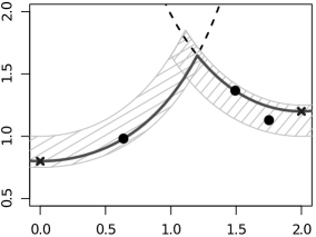
Figure 1: The event $\Delta_{m}$ in the proof of Thm. 3.1. Black crosses: data $(t_{i},Z(t_{i}))$ with $t_{1}=0$ and $t_{2}=2$, black line: $K_{\mathbf{t},Z(\mathbf{t})}$, grey hatched area: $K^{(m)}_{\mathbf{t},Z(\mathbf{t})}$, black dots: $\Pi\cap K_{\mathbf{t},Z(\mathbf{t})}^{(m)}$.
Left: $|\Pi\cap K_{\mathbf{t},Z(\mathbf{t})}^{(m)}\setminus\Pi_{2}|>0$. Right: $|\Pi\cap I_{\{1\}}(Z(\mathbf{t}))|=1>0=|\Pi\cap I_{\{1\}}^{(m)}(Z(\mathbf{t}))|$.

Theorem 3.1

For $\mathbb{P}_{Z(\mathbf{t})}$-a.e. $\mathbf{z}>\mathbf{0}$, we have

$$1.{}\ \mathbb{P}(E_{\mathbf{n}}(Z(\mathbf{t}))\mid Z(\mathbf{t})=\mathbf{z}){}={}\lim_{m\to\infty}\mathbb{P}(E^{(m)}_{\mathbf{n}}(\mathbf{z})\mid Z(\mathbf{t})\in A_{m}(\mathbf{z}))\textrm{ for all }\mathbf{n}\in N_{1},$$

$$2.{}\ \mathbb{P}\big{(}|\Pi_{2}\cap B_{j}|=r_{j},\,1\leq j\leq k,\ |\Pi_{3}\cap B_{j}|=r_{j},\ k<j\leq l\ \big{|}\ Z(\mathbf{t})=\mathbf{z}\big{)}$$

$${}={}\lim_{m\to\infty}\mathbb{P}\big{(}|\Pi\cap K_{\mathbf{t},\mathbf{z}}^{(m)}\cap B_{j}|=r_{j},\ 1\leq j\leq k,$$

$$\hskip 51.21504pt|\Pi\cap B_{j}\setminus(K_{\mathbf{t},\mathbf{z}}^{(m)}\cup\overline{K_{\mathbf{t},\mathbf{z}}}^{(m)})|=r_{j},\ k<j\leq l\ \big{|}\ Z(\mathbf{t})\in A_{m}(\mathbf{z})\big{)}$$

$$\quad\textrm{for any }B_{j}\subset S,\ r_{j}\in\mathbb{N}_{0},\ j\in\{1,\ldots,l\}.$$

Proof

For the proof of the first part, note that, by Lévy’s “Upward” Theorem

$$\mathbb{P}(E_{\mathbf{n}}(Z(\mathbf{t}))\mid Z(\mathbf{t})=\mathbf{z}){}={}\lim\nolimits_{m\to\infty}\mathbb{P}(E_{\mathbf{n}}(Z(\mathbf{t}))\mid Z(\mathbf{t})\in A_{m}(\mathbf{z}))$$

for $\mathbb{P}_{Z(\mathbf{t})}$-a.e. $\mathbf{z}>\mathbf{0}$ and all $\mathbf{n}\in N_{1}$. Thus, as $\mathbb{P}(E^{(m)}_{\mathbf{n}}(Z(\mathbf{t}))\mid Z(\mathbf{t})\in A_{m}(\mathbf{z}))$ equals $\mathbb{P}(E^{(m)}_{\mathbf{n}}(\mathbf{z})\mid Z(\mathbf{t})\in A_{m}(\mathbf{z}))$ by definition, it remains to verify

$$\lim_{m\to\infty}\big{|}\mathbb{P}(E^{(m)}_{\mathbf{n}}(Z(\mathbf{t}))\,|\,Z(\mathbf{t})\in A_{m}(\mathbf{z}))-\mathbb{P}(E_{\mathbf{n}}(Z(\mathbf{t}))\,|\,Z(\mathbf{t})\in A_{m}(\mathbf{z}))\big{|}=0.$$ (8)

To this end, we consider the symmetric difference $\Delta_{m}$ of $E^{(m)}_{\mathbf{n}}(Z(\mathbf{t}))$ and $E_{\mathbf{n}}(Z(\mathbf{t}))$. Note that any element of $\Delta_{m}$ satisfies $|\Pi\cap K_{\mathbf{t},Z(\mathbf{t})}^{(m)}\setminus\Pi_{2}|>0$ or $|\Pi\cap I_{A}(Z(\mathbf{t}))|>|\Pi\cap I_{A}^{(m)}(Z(\mathbf{t}))|$ for some $A\in\mathcal{A}$ (cf. Figure 1). The second kind of event happens if there is a point of $\Pi$ in $I_{A}(Z(\mathbf{t}))\cap(\bigcup_{j\notin A}K_{t_{j},Z(t_{j})}^{(m)})$. As this set vanishes for any $Z(\mathbf{t})>\mathbf{0}$ as $m\to\infty$, we get that

$$U_{A}^{(m)}=\{\omega\in\Omega:\ |\Pi\cap I_{A}(Z(\mathbf{t}))|>|\Pi\cap I_{A}^{(m)}(Z(\mathbf{t}))|\}\searrow\emptyset,\quad m\to\infty,$$

for any $A\in\mathcal{A}$, and therefore $\textstyle\lim_{m\to\infty}\mathbb{P}(U_{A}^{(m)})=0$. This yields

$$\int_{(0,\infty)^{n}} \lim_{m\to\infty}\mathbb{P}\left(U_{A}^{(m)}\,\big{|}\,Z(\mathbf{t})\in A_{m}(\mathbf{z})\right)\mathbb{P}(Z(\mathbf{t})\in\mathrm{d}\mathbf{z})=0$$

by dominated convergence and the fact that

$$\int_{(0,\infty)^{n}}\mathbb{P}\left(U_{A}^{(m)}\ \big{|}\ Z(\mathbf{t})\in A_{m}(\mathbf{z})\right)\mathbb{P}(Z(\mathbf{t})\in\mathrm{d}\mathbf{z})$$

$$={} \textstyle\sum_{\mathbf{z}\in(2^{-m}\mathbb{N})^{n}}\mathbb{P}\left(U_{A}^{(m)}\ \big{|}\ Z(\mathbf{t})\in A_{m}(\mathbf{z})\right)\cdot\mathbb{P}(Z(\mathbf{t})\in A_{m}(\mathbf{z})){}={}\mathbb{P}\big{(}U_{A}^{(m)}\big{)}.$$

Therefore, we have

$$\lim_{m\to\infty}\mathbb{P}\left(|\Pi\cap I_{A}(Z(\mathbf{t}))|>|\Pi\cap I_{A}^{(m)}(\mathbf{z})|\ \big{|}\ Z(\mathbf{t})\in A_{m}(\mathbf{z})\right)=0$$ (9)

for any $A\in\mathcal{A}$ and $\mathbb{P}_{Z(\mathbf{t})}$-a.e. $\mathbf{z}>\mathbf{0}$. All in all, we end up with

$$\lim_{m\to\infty}\Big{|}\mathbb{P}\left(E^{(m)}_{\mathbf{n}}(Z(\mathbf{t}))\ \big{|}\ Z(\mathbf{t})\in A_{m}(\mathbf{z})\right)-\mathbb{P}\left(E_{\mathbf{n}}(Z(\mathbf{t}))\ \big{|}\ Z(\mathbf{t})\in A_{m}(\mathbf{z})\right)\Big{|}$$

$$\leq{} \quad\lim_{m\to\infty}\sum_{A\in\mathcal{A}}\mathbb{P}\left(U_{A}^{(m)}\,\big{|}\,Z(\mathbf{t})\in A_{m}(\mathbf{z})\right)$$

$$+\lim_{m\to\infty}\mathbb{P}\left(|\Pi\cap K^{(m)}_{\mathbf{t},\mathbf{z}}\setminus\Pi_{2}|>0\,\big{|}\,Z(\mathbf{t})\in A_{m}(\mathbf{z})\right){}={}0$$

by (9) and by the second part of Lemma 3. Thus, we get (8).

For the proof of the second assertion, let $B_{1},\ldots,B_{k},B_{k+1},\ldots,B_{l}\subset S$ be Borel sets. Then, each of the events

$$\{|\Pi_{2}\cap B_{j}|\neq|\Pi\cap K_{\mathbf{t},Z(\mathbf{t})}^{(m)}\cap B_{j}|\textrm{ for any }j=1,\ldots,k\}$$

and $$\{|\Pi_{3}\cap B_{j}|\neq|\Pi\cap B_{j}\setminus(K_{\mathbf{t},Z(\mathbf{t})}^{(m)}\cup\overline{K_{\mathbf{t},Z(\mathbf{t})}}^{(m)})|\textrm{ for any }j=k+1,\ldots,l\}$$

implies that $|\Pi\cap K_{\mathbf{t},Z(\mathbf{t})}^{(m)}\setminus\Pi_{2}|>0$. Hence, by the second part of Lemma 3,

$$\lim_{m\to\infty} \Big{|}\mathbb{P}\big{(}|\Pi_{2}\cap B_{j}|=r_{j},\,1\leq j\leq k,\,|\Pi_{3}\cap B_{j}|=r_{j},\,k<j\leq l\,\big{|}\,Z(\mathbf{t})\in A_{m}(\mathbf{z})\big{)}$$

$$\hskip 19.91684pt-\mathbb{P}\big{(}|\Pi\cap K^{(m)}_{\mathbf{t},\mathbf{z}}\cap B_{j}|=r_{j},\ 1\leq j\leq k,$$

$$\hskip 42.67912pt|\Pi\cap B_{j}\setminus(K^{(m)}_{\mathbf{t},\mathbf{z}}\cup\overline{K_{\mathbf{t},\mathbf{z}}}^{(m)})|=r_{j},\ k<j\leq l\,\big{|}\,Z(\mathbf{t})\in A_{m}(\mathbf{z})\big{)}\Big{|}$$

$$\leq{} \lim_{m\to\infty}\mathbb{P}\left(|\Pi\cap K^{(m)}_{\mathbf{t},\mathbf{z}}\setminus\Pi_{2}|>0\ \big{|}\ Z(\mathbf{t})\in A_{m}(\mathbf{z})\right)=0.$$

for any $r_{1},\ldots,r_{k}$, $r_{k+1},\ldots,r_{l}\in\mathbb{N}_{0}$. ∎

We note that there exists a more general version of Theorem 3.1 which we will need for simulation. Let $B_{1},\ldots,B_{k}\in\mathcal{B}^{d}\times((0,\infty)\cap\mathcal{B})\times\mathcal{G}$ be pairwise disjoint with $\bigcup_{j=1}^{k}B_{j}=S$. We introduce generalized “blurred” scenarios

$$E^{(m)}_{\mathbf{n},\mathbf{B}}(\mathbf{z}){}={} \{|\Pi\cap I_{A}^{(m)}(\mathbf{z})\cap B_{j}|=n_{A}^{(j)},\,A\in\mathcal{A},\,1\leq j\leq k,\,|\Pi\cap\overline{K_{\mathbf{t},\mathbf{z}}}^{(m)}|=0\}$$

where $\mathbf{n}=(n_{A}^{(j)})_{A\in\mathcal{A},\ j=1,\ldots,k}\in\mathbb{N}_{0}^{(2^{n}-1)k}$ satisfies $\sum_{j=1}^{k}\sum_{A:\,A\ni i}n_{A}^{(j)}\geq 1$ for all $i\in\{1,\ldots,n\}$. Analogously, generalized scenarios $E_{\mathbf{n},\mathbf{B}}(\mathbf{z})$ are defined. Then, in the same way as Theorem 3.1 the following theorem can be shown.

Theorem 3.2

For $\mathbb{P}_{Z(\mathbf{t})}$-a.e. $\mathbf{z}>\mathbf{0}$, we have

$$\textstyle\mathbb{P}(E_{\mathbf{n},\mathbf{B}}(Z(\mathbf{t}))\mid Z(\mathbf{t})=\mathbf{z})={}\lim_{m\to\infty}\mathbb{P}(E^{(m)}_{\mathbf{n},\mathbf{B}}(\mathbf{z})\mid Z(\mathbf{t})\in A_{m}(\mathbf{z}))$$

for any scenario $E_{\mathbf{n},\mathbf{B}}(\mathbf{z})$ with $\sum_{j=1}^{k}\sum_{A:\,A\ni i}n_{A}^{(j)}\geq 1$ for all $i\in\{1,\ldots,n\}$.

By a straightforward application of Theorems 3.1 and 3.2 the conditional independence of $\Pi_{1}$, $\Pi_{2}$ and $\Pi_{3}$ can be shown and the conditional distribution of $\Pi_{3}$ can be calculated. We skip the proof and refer to Dombry and Eyi-Minko (2013), Thm. 3.1, who obtained these results by a different approach, using Palm theory. However, as Palm theory is not helpful for the calculation of the distribution of $\Pi_{2}$, we use the approximation method for all the results.

Corollary 2

1. With probability one the point processes $\Pi_{1}$, $\Pi_{2}$ and $\Pi_{3}$ conditional on $Z(\mathbf{t})$ are stochastically independent.

2. The process $\Pi_{3}\mid Z(\mathbf{t})=\mathbf{z}$ has the same distribution as $\Pi\setminus(K_{\mathbf{t},\mathbf{z}}\cup\overline{K_{\mathbf{t},\mathbf{z}}})$ for $\mathbb{P}_{Z(\mathbf{t})}$-a.e. $\mathbf{z}>\mathbf{0}$.

By the second part of Corollary 2 the process $\Pi_{3}\mid Z(\mathbf{t})=\mathbf{z}$ can be easily simulated by unconditionally simulating $\Pi$ and restricting it to $\mathbb{R}^{d}\times(0,\infty)\times G\setminus(K_{\mathbf{t},\mathbf{z}}\cup\overline{K_{\mathbf{t},\mathbf{z}}})$.

Remark 1

Note that, by the definition of $\Lambda$ in (2), the process $Z$ in (1) is stationary. Replacing the Lebesgue measure $\mu$ by an arbitrary absolutely continuous measure yields non-stationary models, as well. All the results presented so far still hold true for these processes. The formulae that will occur in Section 4 have to be modified using the corresponding Lebesgue density in case of non-stationarity. The assumption that the distribution of the shape function does not depend on the other components of $\Pi$, however, is crucial. That is, the law of the shape function is independent of the shifting and scaling.

The remainder of the paper will address the problem of simulating $\Pi_{2}\mid Z(\mathbf{t})=z$. We propose a procedure consisting of two steps. First, we draw a scenario $E_{\mathbf{n}}(Z(\mathbf{t}))$ conditional on $Z(\mathbf{t})=\mathbf{z}$. Then, the points of $\Pi_{2}$ corresponding to this scenario are simulated.

4 Results in the case of a finite number of shape functions on the real axis

As shown in Section 3, the calculation of $\mathbb{P}(E_{\mathbf{n}}(Z(\mathbf{t}))\mid Z(\mathbf{t})=\mathbf{z})$ requires knowledge about the exact asymptotic behaviour of $\Lambda(I_{A}^{(m)}(\mathbf{z}))$. In particular, the behaviour of the intersection of two curves $K_{t_{i},z_{i}+\delta_{i}}\cap K_{t_{j},z_{j}+\delta_{j}}$ for small $|\delta_{i}|$ and $|\delta_{j}|$ needs to be analysed. Explicit calculations turn out to be quite laborious. Therefore, we restrict ourselves to the case $d=1$. We calculate the asymptotics of $\Lambda(I_{A}^{(m)}(\mathbf{z}))$ for $|A|=1$ (Proposition 5), $|A|=2$ (Proposition 2) and $|A|\geq 3$ (Proposition 3), see Figure 2. In the case $|A|\geq 3$, the rate of convergence of $\Lambda(I_{A}^{(m)})$ cannot be determined exactly. Nevertheless, the conditional probability of any scenario can be calculated (Theorem 4.1). All the proofs of this section are postponed to Section 10.

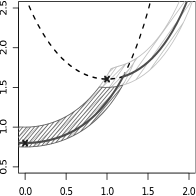
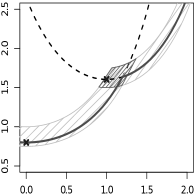
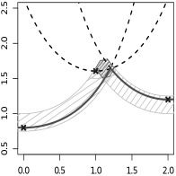
Figure 2: Blurred intersection sets for $|A|=1$, $|A|=2$ and $|A|=3$. Black crosses: data $(t_{i},Z(t_{i}))$, dashed black lines: $K_{t_{i},Z(t_{i})}$, black line: $K_{\mathbf{t},Z(\mathbf{t})}$, grey hatched area: $K^{(m)}_{\mathbf{t},Z(\mathbf{t})}$, black hatched area: $I_{A}^{(m)}(Z(\mathbf{t}))$ with $|A|=1$ (left), $|A|=2$ (middle) and $|A|=3$ (right).

First we assume that $G$ is a finite space of functions $f:\mathbb{R}\to[0,\infty)$ such that the intersections

$$M_{c,t_{0}}=\{t\in\mathbb{R}:\ f(t)=cf(t_{0}+t),\ f(t)>0\}$$ (10)

are finite for all $c>0$, $t_{0}\in\mathbb{R}$, $f\in G$. This implies that each set $I_{A}(\mathbf{z})$, $A\in\mathcal{A}$, $|A|\geq 2$, $\mathbf{z}>\mathbf{0}$, is finite. Without loss of generality, we assume that $\mathbb{P}_{F}(\{f\})>0$ for all $f\in G$.

The following Propositions 2 and 3, deal with the asymptotic behaviour of $\Lambda(I^{(m)}_{A}(\mathbf{z}))$, $|A|>1$, as $m\to\infty$. For simplicity, we assume that $I_{A}(\mathbf{z})$ consists of a single point. In general, $I_{A}(\mathbf{z})$ is finite and, for $m$ large enough, $I_{A}^{(m)}(\mathbf{z})$ consists of $|I_{A}(\mathbf{z})|$ disjoint components. Thus, $\Lambda(I^{(m)}_{A}(\mathbf{z}))$ is the sum of the measures belonging to each component (cf. Remark 2 and Proposition 4).

Proposition 2

Let $t_{1},t_{2}\in\mathbb{R}$, $z_{1},z_{2}>0$ such that $I_{\{1,2\}}(\mathbf{z})=\{(t_{0},y_{0},f)\}.$ Furthermore, let $f$ be continuously differentiable in a neighbourhood of $t_{1}-t_{0}$ and $t_{2}-t_{0}$ with

$$z_{1}f^{\prime}(t_{2}-t_{0})\neq z_{2}f^{\prime}(t_{1}-t_{0}).$$ (11)

Then, we have

$$\Lambda(I_{\{1,2\}}^{(m)}(\mathbf{z}))=\frac{2^{-2m}}{y_{0}^{2}|z_{1}f^{\prime}(t_{2}-t_{0})-z_{2}f^{\prime}(t_{1}-t_{0})|}\mathbb{P}_{F}(\{f\})+o(2^{-2m}).$$

Remark 2

1. Using $\frac{z_{1}}{f(t_{1}-t_{0})}=\frac{z_{2}}{f(t_{2}-t_{0})}=y_{0}$ we get that equality in (11) holds if and only if

   $$\frac{\partial}{\partial t}\frac{z_{1}}{f(t_{1}-t)}\bigg{|}_{t=t_{0}}=\frac{\partial}{\partial t}\frac{z_{2}}{f(t_{2}-t)}\bigg{|}_{t=t_{0}},$$

   i.e. if and only if the two sets of admissible points, $K_{t_{1},z_{1}}$ and $K_{t_{2},z_{2}}$, are tangents to each other in $(t_{0},y_{0},f)$ which is an event of probability zero by Assumption (10). Therefore, (11) is satisfied $\mathbb{P}_{Z(\mathbf{t})}$-a.s.

2. If $I_{\{1,2\}}(z_{1},z_{2})=\{(s_{1},u_{1},f_{1}),\ldots,(s_{k},u_{k},f_{k})\},$ we obtain

   $$\textstyle\Lambda(I^{(m)}_{\{1,2\}}(\mathbf{z}))=2^{-2m}\cdot\sum_{j=1}^{k}\frac{\mathbb{P}_{F}(\{f_{j}\})}{u_{j}^{2}\cdot|z_{1}f_{j}^{\prime}(t_{2}-s_{j})-z_{2}f_{j}^{\prime}(t_{1}-s_{j})|}+o(2^{-2m}).$$

Proposition 3

Let $t_{1},\ldots,t_{l}\in\mathbb{R}$, $z_{1},\ldots,z_{l}>0$, $l\geq 3$ such that $I_{\{1,\ldots,l\}}(\mathbf{z})=\{(t_{0},y_{0},f)\}$ where $f$ is continuously differentiable in a neighbourhood of $t_{1}-t_{0},\ldots,t_{l}-t_{0}$ such that (11) holds for $(t_{1},z_{1})$ and $(t_{2},z_{2})$. Then, we have

$$\Lambda(I_{\{1,\ldots,l\}}^{(m)}(\mathbf{z}))\leq{}\frac{2^{-2m}}{y_{0}^{2}|z_{1}f^{\prime}(t_{2}-t_{0})-z_{2}f^{\prime}(t_{1}-t_{0})|}\mathbb{P}_{F}(\{f\})+o(2^{-2m}).$$

For any $C>0$, $\varepsilon>0$, there exists $m_{C,\varepsilon}\in\mathbb{N}$ such that

$$\Lambda(I_{\{1,\ldots,l\}}^{(m)}(\mathbf{z}))\geq{}C2^{-2m(1+\varepsilon)},\qquad m\geq m_{C,\varepsilon}.$$

Whilst Proposition 3 does not provide exact asymptotics, we get exact results in the following situation.

Proposition 4

Let $I_{\{1,\ldots,l\}}(\mathbf{z})=\{(s_{1},u_{1},f_{1}),\ldots,(s_{k},u_{k},f_{k})\}$, $l\geq 3$, where $f_{1},\ldots,f_{k}:\mathbb{R}\to[0,\infty)$ are continuously differentiable in a neighbourhood of $t_{i}-s_{j}$, $i=1,\ldots,l$, $j=1,\ldots,k$ such that (11) holds for $(t_{1},z_{1})$, $(t_{2},z_{2})$ and each $(s_{j},y_{j},f_{j})$, $j=1,\ldots,k$. Then, we have

$$\mathbb{P}((t_{0},y_{0},f)\in\Pi\mid|\Pi\cap I_{\{1,\ldots,l\}}(Z(\mathbf{t}))|=1,\,Z(\mathbf{t})=\mathbf{z})$$

$$= \frac{y_{0}^{-2}\mathbb{P}_{F}(\{f\})}{|z_{1}f^{\prime}(t_{2}-t_{0})-z_{2}f^{\prime}(t_{1}-t_{0})|}\bigg{(}\sum_{j=1}^{k}\frac{u_{j}^{-2}\mathbb{P}_{F}(\{f_{j}\})}{|z_{1}f^{\prime}_{j}(t_{2}-s_{j})-z_{2}f^{\prime}_{j}(t_{1}-s_{j})|}\bigg{)}^{-1}$$ (12)

for $(t_{0},y_{0},f)\in I_{\{1,\ldots,l\}}(\mathbf{z})$. Furthermore, for $\mathbb{P}_{Z(\mathbf{t})}$-a.e. $\mathbf{z}>\mathbf{0}$, the right-hand side of (12) does not depend on the choice of the labelling.

Proposition 5

Let $f\in G$, $\mathbf{t}\in\mathbb{R}^{n}$, $\mathbf{z}>\mathbf{0}$ such that $f$ is continuously differentiable in a neighbourhood of $t_{i}-t_{0}$ for all $i\in\{1,\ldots,n\}$ and all $(t_{0},y_{0},f)\in K_{\mathbf{t},\mathbf{z}}\cap\bigcup_{\begin{subarray}{c}l=1\\ l\neq i\end{subarray}}^{n}(K_{t_{i},z_{i}}\cap K_{t_{l},z_{l}})$, i.e. all $(t_{0},y_{0},f)\in K_{t_{i},z_{i}}$ that generate at least two observations. Furthermore, we denote the projection of the set $I_{\{i\}}(\mathbf{z})\cap(\mathbb{R}\times(0,\infty)\times\{f\})$ onto its first component in $\mathbb{R}$ by

$$D_{i}^{(f)}=\{t\in\mathbb{R}:\ (t,y,f)\in I_{\{i\}}(\mathbf{z})\textrm{ for some }y>0\}.$$

Then, with $S_{f}=\mathbb{R}\times(0,\infty)\times\{f\}$, we have

$$\Lambda\left(I_{\{i\}}^{(m)}(\mathbf{z})\cap S_{f}\right)={}2^{-m}\cdot\mathbb{P}_{F}(\{f\})\cdot z_{i}^{-2}\int_{D_{i}^{(f)}}f(t_{i}-t)\,\mathrm{d}t+o(2^{-m}).$$ (13)

We can use Theorem 3.1 in order to compute the conditional probabilities

$$\mathbb{P}(E_{\mathbf{n}}(Z(\mathbf{t}))\mid Z(\mathbf{t})=\mathbf{z})={} \lim_{m\to\infty}\frac{\mathbb{P}(E^{(m)}_{\mathbf{n}}(\mathbf{z}))}{\sum_{\tilde{\mathbf{n}}\in N_{0}}\mathbb{P}(E^{(m)}_{\tilde{\mathbf{n}}}(\mathbf{z}))}$$ (14)

where $N_{0}=\{(n_{A})_{A\in\mathcal{A}}:\ \sum_{A:\,A\ni i}n_{A}=1,\ i=1,\ldots,n\}$.

As the sets $I_{A}^{(m)}(\mathbf{z})$, $A\in\mathcal{A}$, are pairwise disjoint and $\Lambda(I_{A}^{(m)}(\mathbf{z}))$ tends to zero for $m\to\infty$ by Lemma 1, we get

$$\mathbb{P}(E^{(m)}_{\mathbf{n}}(\mathbf{z}))\sim{} \textstyle\exp(-\Lambda(\overline{K_{\mathbf{t},\mathbf{z}}}))\prod_{A:\,n_{A}=1}\Lambda(I_{A}(\mathbf{z})).$$ (15)

Considering (14), we can restrict ourselves to those scenarios with the slowest rate of convergence to zero. Propositions 2, 3 and 5 yield that scenarios involving intersections of at least three sets are always of a dominating order. Therefore, all unknown terms from Proposition 3 appear as factors in the numerator and denominator in (14) and hence are cancelled out. Using the formulae above, the limits of the conditional probabilities can always be calculated explicitly except for those cases where two scenarios exist, both involving different terms which cannot be determined exactly (cf. Proposition 3). This may happen only if two sets $A_{1}=\{i_{1},\ldots,i_{r}\}$ and $A_{2}=\{j_{1},\ldots,j_{s}\}$, $r,s\geq 3$, $A_{1}\cap A_{2}\neq\emptyset$, exist such that

$$J_{A_{1}}(Z(\mathbf{t}))\neq\emptyset\ ,\ J_{A_{2}}(Z(\mathbf{t}))\neq\emptyset\textrm{ and }J_{A_{1}\cup A_{2}}(Z(\mathbf{t}))=\emptyset,$$ (16)

where $J_{A}(Z(\mathbf{t}))=\bigcup_{B\supset A}I_{B}(Z(\mathbf{t}))=K_{\mathbf{t},Z(\mathbf{t})}\cap\bigcap_{i\in A}K_{t_{i},Z(t_{i})}$, $A\in\mathcal{A}$.

In all other cases the terms as in Proposition 3 are cancelled out. Note that we work with sets of the type $J_{A}(Z(\mathbf{t}))$ in order to avoid case-by-case analysis for all the sets $I_{B}(Z(\mathbf{t}))$ with $B\supset A$.

Lemma 4

Let $G$ consist of functions which are continuously differentiable a.e. Then, for any fixed set $\{t_{1},\ldots,t_{n}\}\subset\mathbb{R}$ we have

$$\mathbb{P}(Z(\mathbf{t})\textrm{ satisfies }\eqref{eq:problems})=0.$$

Thus, from the considerations above we directly derive the following result.

Theorem 4.1

Let $G$ be a finite set of functions which are continuously differentiable a.e. Then, for $\mathbb{P}_{Z(\mathbf{t})}$-a.e. $\mathbf{z}>\mathbf{0}$,

$$\mathbb{P}(E_{\mathbf{n}}(Z(\mathbf{t}))\mid Z(\mathbf{t})=\mathbf{z}){}={} \lim_{m\to\infty}\mathbb{P}(E^{(m)}_{\mathbf{n}}(\mathbf{z})\mid Z(\mathbf{t})\in A_{m}(\mathbf{z}))$$

can be calculated explicitly by the results of Propositions 2, 3, 4 and 5.

Remark 3

We may also consider the case that $G$ is countable. However, to transfer the results of the finite case, we have to ensure uniform convergence of the blurred intersection sets which is needed to compute the term $\sum_{\mathbf{n}\in N_{0}}\mathbb{P}(E^{(m)}_{\mathbf{n}}(\mathbf{z}))$ in the denominator of Equation (14). To this end, we have to impose some additional conditions. For example, we could assume that for almost every $\mathbf{z}>\mathbf{0}$ there is only a finite number of shape functions involved in the intersection sets $I_{A}(\mathbf{z})$, $|A|\geq 2$.

We are still left with simulating $\Pi_{2}\mid Z(\mathbf{t})=\mathbf{z}$ given the occurrence of a scenario $E_{\mathbf{n}}(\mathbf{z})$ with $\mathbf{n}\in N_{0}$, that is, we are interested in

$$\textstyle\mathbb{P}\left(\bigcap_{A:\,n_{A}=1}\{|\Pi_{2}\cap(C_{A}\times(0,\infty)\times\{f\})|=1\}\ \big{|}\ E_{\mathbf{n}}(\mathbf{z})\right)$$

for $C_{A}\subset\mathbb{R}$, $f\in G$ with $(C_{A}\times(0,\infty)\times\{f\})\cap I_{A}(\mathbf{z})\neq\emptyset$. Using Theorem 3.2 with sets $B_{A}=C_{A}\times(0,\infty)\times\{f\}$, $A\in\mathcal{A}$, we get that

$$\mathbb{P}\bigg{(}\bigcap_{A:n_{A}=1}\{|\Pi_{2}\cap I_{A}(\mathbf{z})\cap B_{A}|=1\}\,\big{|}\,E_{\mathbf{n}}(\mathbf{z})\bigg{)}=\lim_{m\to\infty}\prod_{A:n_{A}=1}\frac{\Lambda(I_{A}^{(m)}(\mathbf{z})\cap B_{A})}{\Lambda(I_{A}^{(m)}(\mathbf{z}))}.$$

Thus, each point of $\Pi_{2}$ can be simulated independently. If $\Pi_{2}\cap I_{A}(Z(\mathbf{t}))$ contains exactly one point, define $T_{A}\in\mathbb{R}$ and $F_{A}\in G$ such that

$$\Pi_{2}\cap I_{A}(Z(\mathbf{t}))=\{(T_{A},F_{A}(t_{i^{*}}-T_{A})/Z(t_{i^{*}}),F_{A})\}$$ (17)

for any arbitrary $i^{*}\in A$. Note that the distribution of $(T_{A},F_{A})$ depends on the cardinal number of $A$. If $A=\{i\}$ for some $i\in\{1,\ldots,n\}$, we have

$$\mathbb{P}(T_{A}\in B,F_{A}=f)=\frac{\mathbb{P}_{F}(\{f\})\int_{D_{i}^{(f)}\cap B}f(t_{i}-t)\,\mathrm{d}t}{\sum_{g\in G}\mathbb{P}_{F}(\{g\})\int_{D_{i}^{(g)}}g(t_{i}-t)\,\mathrm{d}t},\quad B\in\mathcal{B}.$$

For $|A|\geq 2$, let $I_{A}(\mathbf{z})=\{(s_{1},u_{1},f_{1}),\ldots,(s_{k},u_{k},f_{k})\}$. Then, we get

$$\mathbb{P}(T_{A}=s_{j},F_{A}=f_{j})=\frac{\frac{u_{j}^{-2}\mathbb{P}_{F}(\{f_{j}\})}{|z_{1}f^{\prime}_{j}(t_{2}-s_{j})-z_{2}f^{\prime}_{j}(t_{1}-s_{j})|}}{\sum_{l=1}^{k}\frac{u_{l}^{-2}\mathbb{P}_{F}(\{f_{l}\})}{|z_{1}f^{\prime}_{l}(t_{2}-s_{l})-z_{2}f^{\prime}_{l}(t_{1}-s_{l})|}},\quad 1\leq j\leq k.$$

Thus, we end up with the following procedure for calculating the conditional distribution of $Z(\cdot)$ given $Z(\mathbf{t})$ with $t_{1},\ldots,t_{n}\in\mathbb{R}$, $\mathbf{z}>\mathbf{0}$.

1. Compute the conditional probabilities (14) for all the scenarios $E_{\mathbf{n}}(\mathbf{z})$ and generate a random scenario following this distribution.

2. For a given scenario $E_{\mathbf{n}}(\mathbf{z})$ simulate $\Pi_{2}=\{(T_{A},\frac{z_{i^{*}}}{F_{A}(t_{i^{*}}-T_{A})},F_{A}):\ n_{A}=1\}$ for an arbitrary $i^{*}\in A$. Here, the law of $(T_{A},F_{A})$ is given above.

3. Independently, sample from $\Pi_{3}=\Pi\cap(\mathbb{R}\times(0,\infty)\times G)\setminus(K_{\mathbf{t},\mathbf{z}}\cup\overline{K_{\mathbf{t},\mathbf{z}}})$.
   Then, $Z(\cdot)=\max_{(s,u,f)\in\Pi_{2}\cup\Pi_{3}}uf(\cdot-s)$.

In the next section, we will demonstrate the performance of this exact approach by comparing it to other algorithms in the simple case of a deterministic, continuously differentiable shape function.

5 Comparison with the algorithms for the max-linear model and for Gaussian processes with transformed marginals

Recently, Wang and Stoev (2011) proposed an algorithm for exact and efficient conditional sampling for max-linear models

$$Z(t_{i})=\max_{j=1,\ldots,p}a_{ij}Y_{j},\quad i=0,\ldots,n,$$

where $Y_{j},\ j=1,\ldots,p,$ are independent standard Fréchet random variables. With the representation (3) of $Z$ as an extremal integral we see that $Z$ can be approximated arbitrarily well by a max-linear model, e.g. by

$$Z_{M,h}(t)=h\max_{\begin{subarray}{c}l=-M,\ldots,M-1\\ j=1,\ldots,k\end{subarray}}\mathbb{P}_{F}(\{f_{j}\})\cdot f_{j}\Big{(}t-\Big{(}l+\frac{1}{2}\Big{)}h\Big{)}\cdot Y_{j,l},\quad M\in\mathbb{N},\ h>0,$$

where $G=\{f_{1},\ldots,f_{k}\}$. Then, we have $Z_{M,h}(t)\stackrel{{\scriptstyle P}}{{\longrightarrow}}Z(t)$ for any $t\in\mathbb{R}$ as $M\to\infty$, $h\to 0$.

We also consider another approach based on the assumption of a multi-Gaussian model (cf. Chilès and Delfiner, 1999, p. 381). The data are transformed such that the marginal distribution is Gaussian. As the marginals of $Z$ are standard Fréchet, the corresponding transformation is given by

$$\Psi:(0,\infty)\to\mathbb{R},\ x\mapsto\Phi^{-1}(\Phi_{1}(x)),$$

where $\Phi$ is the standard normal distribution function and $\Phi_{1}=\exp(-1/x)$ is the standard Fréchet distribution function. The transformed random field $Y=\Psi(Z)$ is stationary and has second-order moments. As the computation of covariance function $C$ of $Y$ for general shape functions $f_{1},\ldots,f_{k}$ is complex, we estimate $C$ using maximum likelihood techniques, for instance, from a convenient parametric class such as the Whittle-Matérn class, i.e.

$$C_{\nu,c}(h)=\frac{(c||h||)^{\nu}}{2^{\nu-1}\Gamma(\nu)}\mathcal{K}_{\nu}(c||h||),\quad\nu,\ c>0,$$ (18)

assuming that $Y$ is a Gaussian random field. Under this assumption, the conditional distribution can be sampled easily (see Lantuéjoul, 2002, for instance). Afterwards, the sample has to be retransformed via

$$\Psi^{-1}:\mathbb{R}\to(0,\infty),\ y\mapsto\Phi_{1}^{-1}(\Phi(y)).$$

Note that, in general, this procedure is not exact as $Y$ is not a Gaussian random field, but only marginally Gaussian.

To compare these different methods, we need a measure for the goodness-of-fit of a distribution. Here, we use the continuous ranked probability score (CRPS) which is defined as

$$CRPS(F_{1},x)=-\int_{-\infty}^{\infty}(F_{1}(y)-\mathbf{1}_{\{y\geq x\}})^{2}\,\mathrm{d}y,$$

where $F_{1}$ is a cumulative distribution function and $x\in\mathbb{R}$ (Gneiting and Raftery, 2007). Note that $CRPS(F_{1},F_{2}):=\int CRPS(F_{1},x)F_{2}({\rm d}x)$ is a strictly proper scoring rule, i.e.

$$CRPS(F_{2},F_{2})\geq CRPS(F_{1},F_{2})$$

for all cumulative distribution functions $F_{1}$, $F_{2}$. If both $F_{1}$ and $F_{2}$ belong to measures with finite first moment, equality holds if and only if $F_{1}=F_{2}$. Assuming that $F_{1}$ has a finite first moment, the CRPS can be calculated via

$$CRPS(F_{1},x)=\frac{1}{2}\mathbb{E}|X-X^{\prime}|-\mathbb{E}|X-x|,$$ (19)

which shows that $CRPS(F_{1},F_{1})=-\frac{1}{2}\mathbb{E}|X-X^{\prime}|\leq 0$. Here, $X$, $X^{\prime}\sim F_{1}$ are independent random variables.

In order to compare different algorithms that simulate from the conditional distribution $\log(Z(t_{0}))\mid Z(\mathbf{t})$, we consider $K$ samples $Z_{1},\ldots,Z_{K}$ of the random field $Z$. For each method, we get an empirical distribution function $F_{i}$ as the (approximated) conditional distribution of $\log(Z_{i}(t_{0}))\mid Z_{i}(\mathbf{t})$, $i=1,\ldots,K$, and calculate $CRPS(F_{i},\log(Z_{i}(t_{0})))$ via (19). Here, we do the $\log$-transformation to Gumbel marginals to ensure that the conditional distribution has finite expectation.

Then, a measure for the goodness-of-fit is given by the mean score (Gneiting and Raftery, 2007)

$$\textstyle CRPS_{K}=\frac{1}{K}\sum_{i=1}^{K}CRPS(F_{i},\log(Z_{i}(t_{0}))).$$

Further, we have a look at the mean absolute error of the conditional median

$$\textstyle MAE_{K}=\frac{1}{K}\sum_{i=1}^{K}\left|F_{i}^{-1}(0.5)-\log(Z_{i}(t_{0}))\right|.$$

For computational reasons, we choose Smith’s (1990) process with the deterministic shape function

$$f(x)=\varphi(x)=(2\pi)^{-1/2}\exp\left(-x^{2}/2\right).$$

Furthermore, let $n=4$, $\mathbf{t}=(-2,-1,1,2)$ and $t_{0}=0$. Figure 3 shows two realizations of $Z(\cdot)$, the first one is sampled unconditionally and the second one is based on conditional sampling of the first one.

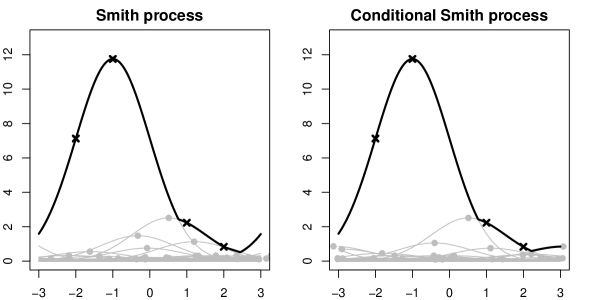
Figure 3: Left: Construction of $Z$. The grey dots represent the points $(s,u\cdot f(0))$ with $(s,u,f)\in\Pi$, the black line is one realization of $Z$. The black dots mark $Z(\mathbf{t})$. Right: Construction of $Z$ conditional on $Z(\mathbf{t})$.

The conditional distribution is calculated based on a sample of size $100$ simulated in R (Ihaka and Gentleman, 1996). The performance is measured via $CRPS_{K}$ and $MAE_{K}$ for the methods $PPP$ (conditional sampling via the Poisson point process), $MLM$ (conditional sampling for a max-linear model with $M=5$ and $h=0.1$ using the R package maxLinear (Wang, 2010)) and $GPT$ (conditional sampling of a Gaussian process with transformed Fréchet marginals) with $K=1000$ samples. As already mentioned, the last approach requires the knowledge of the covariance structure of the transformed random field. This is assessed by first simulating data from this model on a dense grid repeatedly and then estimating the parameters of a Whittle-Matérn covariance model based on maximum likelihood techniques implemented in the R package RandomFields (Schlather, 2013).

The parameters are chosen such that of the first and second method have a similar running time. For these parameters, $GPT$ runs much faster than $PPP$ and $MLM$. In general, however, the running times scale differently in the number $n$ of observations as well as in the number of shape functions. The running time of $PPP$ grows linearly in the number of shape functions and exponentially in $n$. Making use of some conditional independence structure, Wang and Stoev (2011) could improve the complexity of their algorithm. Thus, the running time of $MLM$ depends linearly on both $p$ (which is a multiple of the number of shape functions) and $n$ as Wang and Stoev (2011) report. The complexity of the last method, $GPT$, only depends on $n$ and is of order $\mathcal{O}(n^{3})$ as the conditional expectation and variance of the (marginally) Gaussian distribution has to be calculated.

Table 1: Results of the simulation study for $f(x)=\varphi(x)$ and $K=1000$.

	$PPP$	$MLM$	$GPT$
$CRPS_{K}$	-0.135	-0.359	-0.251
$MAE_{K}$	0.197	0.506	0.338

The results of the simulation study are shown in Table 1. Here, $CRPS_{K}$ and $MAE_{K}$ for $PPP$ can be interpreted as reference values as the first method is exact. We note that conditional sampling for max-linear models performs worse than conditional sampling via transformation to Gaussian marginals.

For further analysis and comparison of these methods we do not restrict ourselves to pointwise prediction, but have a look at the sample paths. Additionally, pointwise quantile estimation of the conditional distribution can be done including the special case of the conditional median which can be seen as an analogue to kriging (Chilès and Delfiner, 1999). In case of conditional sampling via the Poisson point process and conditional sampling of a max-linear model the quantiles have to be estimated from the empirical conditional distribution. For sampling via Gaussian processes the quantiles can be calculated from the kriged value and the kriging variance.

Figure 4 shows five sample paths and the median of the Smith process on

1. observations at four locations $-2$, $-1$, $1$, $2$,

2. observations at eleven locations $-2.5,-2,\ldots,2,2.5$.

In general, conditional simulation via the Poisson point process yields sample paths which capture the main features of the process quite well. Even in the case of four observations parts of the sample path are reconstructed exactly with a positive probability. For eleven observations most of the sample path is restored with high probability.

The results of conditional sampling of the max-linear model are similar to the first method in case of four observations. For eleven observations, however, the method fails because of model misspecification. In the max-linear model, the points generating the observations are assumed to be located on a lattice $h\mathbb{Z}^{d}+\frac{1}{2}$, not at arbitrary locations in $\mathbb{R}^{d}$ as assumed in (1). Due to this restriction, the data do not match the max-linear model and some observations cannot be reconstructed. For some realizations of the Smith process this problem even occurs in case of four observations. This is the main reason for the unsatisfying results of this method in the simulation study above. Note that – as computational experiments show – misspecification most often occurs if at least three observations are generated by the same point. However, for any $h>0$, with probability one, this point is not in $h\mathbb{Z}^{d}+\frac{1}{2}$ and therefore, in these cases, conditional sampling from the max-linear model fails even for small $h$. Thus, although the joint distribution can be approximated arbitrarily well as $h\searrow 0$, the problem of misspecification in the algorithm of Wang and Stoev (2011) is not resolved.

Conditional sampling for Gaussian processes with transformed marginals yields sample paths which are structurally very different from the true ones. However, for eleven observations the deviations from the original sample path are quite small.

a.

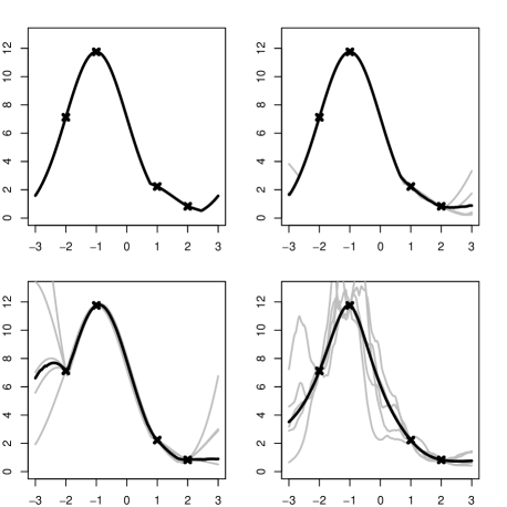
b.

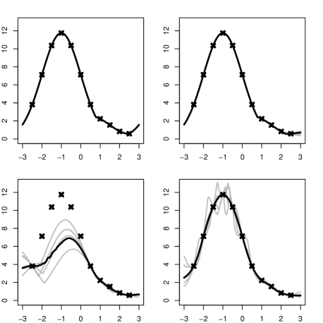
Figure 4: Comparison of the Smith process with different types of conditional simulations: a. simulations conditional on four observations at $-2$, $-1$, $1$, $2$, b. simulations conditional on eleven observations at $-2.5,-2,\ldots,2,2.5$. In both cases the original Smith process (top left), conditional samples via the Poisson point process (top right) and conditional results for a max-linear approximation (bottom left) and an approximation via a Gaussian process with transformed marginals (bottom right) are shown. Black crosses: observations, grey lines: conditional sample paths, black line: conditional median.

Finally, we investigate the behaviour of the different algorithms if the observations are in the tails of the max-stable distribution. Thus, we repeat the simulation study above considering $K=1000$ samples of the random field $Z$ conditional on $\min\{Z(t_{1}),\ldots,Z(t_{n})\}\geq\Phi_{1}^{-1}(q)$. Note that the covariance structure used for $GPT$ is again estimated from transformed samples of the random field $Z$. Besides $GPT$, we also consider an adjusted version ($AGPT$) where the scale parameter $c$ in (18) is estimated based on extreme samples $(Z(t_{1}),\ldots,Z(t_{n}))\mid\min\{Z(t_{1}),\ldots,Z(t_{n})\}\geq\Phi_{1}^{-1}(q)$ and the smoothness parameter $\nu$ is the same as for $GPT$. By this modification of the scale, we account for possible changes of the covariance structure in the extremes. The results of the simulation study for $q=0.9$, $q=0.95$ and $q=0.99$ are shown in Table 2. Note that the probability that all the observations $(t_{1},Z(t_{i}))$, $i=1,\ldots,n$, are generated by the same point tends to one as $q\nearrow 1$ and thus the distribution of $Z(t_{0})\mid Z(\mathbf{t})$ becomes more and more concentrated. Therefore, the CRPS and MAE of the exact algorithm ($PPP$) tend to zero. For Wang and Stoev’s (2011) algorithm, however, the results get worse as $q$ approaches 1. Here, the misspecification issue gets even more problematic as the probability that all the observations are generated by the same point increases. Thus, a large number of data does not match the max-linear model and the algorithm of Wang and Stoev (2011) yields unsatisfactory results. The CRPS and MAE of the algorithm for Gaussian processes with transformed marginals also both get worse as $q$ gets close to 1. This is due to the fact that Gaussian random variables are asymptotically independent. Thus, the algorithm is not able to capture the joint tail behaviour well if we use the the same covariance structure as for the non-extreme observations. For the adjusted version, however, where the modified scale parameter leads to stronger correlations, both the CRPS and the MAE improve as $q$ approaches $1$.

Table 2: Results of the simulation study for the Smith process. CRPS and MAE for the distribution of $Z(t_{0})\mid Z(\mathbf{t})$ based on $K=1000$ samples conditional on $\min Z(\mathbf{t})\geq\Phi_{1}^{-1}(q)$.

		CRPS					MAE
$q$		$PPP$	$MLM$	$GPT$	$AGPT$		$PPP$	$MLM$	$GPT$	$AGPT$
0.90		-0.014	-1.227	-0.338	-0.234		0.016	1.693	0.415	0.284
0.95		-0.006	-1.525	-0.389	-0.196		0.006	2.104	0.491	0.228
0.99		-0.001	-1.901	-0.568	-0.126		0.000	2.611	0.856	0.117

6 Approximation in the case of an infinite number of shape functions

Here, we drop the assumption that $G$ is finite. We present an approximation of the distribution of $Z(\cdot)$ given $Z(\mathbf{t})$ based on a finite number of shape functions. Let $F_{1},F_{2},\ldots$ be independent copies of $F$ where $F$ is defined as in Section 1. Then, given $F_{1},\ldots,F_{N}$, we define

$$\textstyle Z_{N}(t)=\max_{(s,u,f)\in\Pi^{(N)}}uf(t-s),\quad t\in\mathbb{R}^{d},$$ (20)

where $\Pi^{(N)}$ is a Poisson point process on $\mathbb{R}^{d}\times(0,\infty)\times\{F_{1},\ldots,F_{N}\}$ with intensity measure

$$\Lambda(A\times B\times\{F_{k}\})=\frac{1}{N}\int_{A}\int_{B}u^{-2}\,\mathrm{d}u\,\mathrm{d}s,\ A\in\mathcal{B}^{d},\ B\in\mathcal{B}\cap(0,\infty),\ k\in\{1\ldots,n\}.$$

For a proof of the following theorem, see Oesting (2012, Ch. 5).

Theorem 6.1

For any $\mathbf{z}>\mathbf{0}$ we have

$$\Pi^{(N)}\mid Z_{N}(\mathbf{t})\leq\mathbf{z}\stackrel{{\scriptstyle D}}{{\longrightarrow}}\Pi\mid Z(\mathbf{t})\leq\mathbf{z}$$

as $N\to\infty$. In particular, $Z_{N}(\cdot)\mid Z_{N}(\mathbf{t})\leq\mathbf{z}\stackrel{{\scriptstyle D}}{{\longrightarrow}}Z(\cdot)\mid Z(\mathbf{t})\leq\mathbf{z}$ in the sense of finite-dimensional distributions.

If $G$ is countable, we apply the second part of Corollary 2 to the process $Z_{N}$ yielding $\lim_{N\to\infty}\Pi_{3}^{(N)}\mid(Z_{N}(\mathbf{t})=\mathbf{z})\stackrel{{\scriptstyle D}}{{=}}\lim_{N\to\infty}\left(\Pi_{N}\setminus(K_{\mathbf{t},\mathbf{z}}\cup\overline{K_{\mathbf{t},\mathbf{z}}})\right).$ Thus, Theorem 6.1 and the second part of Corollary 2 (applied to $Z$) imply that

$$\lim_{N\to\infty}\Pi_{3}^{(N)}\mid(Z_{N}(\mathbf{t})=\mathbf{z})\stackrel{{\scriptstyle D}}{{=}}{} \Pi\setminus(K_{\mathbf{t},\mathbf{z}}\cup\overline{K_{\mathbf{t},\mathbf{z}}}){}\stackrel{{\scriptstyle D}}{{=}}{}\Pi_{3}\mid(Z(\mathbf{t})=\mathbf{z}).$$

This motivates to improve the approximation $\Pi\approx\Pi^{(N)}$ by $\Pi\approx\Pi_{2}^{(N)}\cup\Pi_{3}$, i.e. by the following procedure:

1. Simulate $\Pi^{(N)}_{2}\mid Z(\mathbf{t})=\mathbf{z}$.

2. Independently of $\Pi_{2}^{(N)}$, sample $\Pi_{3}\mid Z(\mathbf{t})=\mathbf{z}$ defined as $\Pi\cap(\mathbb{R}\times(0,\infty)\times G)\setminus(K_{\mathbf{t},\mathbf{z}}\cup\overline{K_{\mathbf{t},\mathbf{z}}})$ analogously to the second part of Corollary 2.

Then, $Z(\cdot)\approx\max_{(s,u,f)\in\Pi_{2}\cup\Pi_{3}}uf(\cdot-s)$.

7 Application to the Brown-Resnick process

We will apply the method of conditional sampling via the Poisson point process to the process constructed by Brown and Resnick (1977).

Let $\{W_{x}(t),\ t\in\mathbb{R}\}$, $x\in(0,\infty)$, be independent copies of a standard Brownian motion and — independently of the $W_{x}$’s — let $\tilde{\Pi}$ be a Poisson point process on $(0,\infty)$ with intensity measure $u^{-2}\,\mathrm{d}u$. Then,

$$\textstyle Z(t)=\max_{u\in\tilde{\Pi}}\left(u\exp\left(W_{u}(t)-|t|/2\right)\right),\quad t\in\mathbb{R},$$ (21)

defines a stationary max-stable process with standard Fréchet margins.

Recently, this process was generalized (Kabluchko et al, 2009) yielding a class of processes which essentially corresponds to the class of processes that occur as the limit of maxima of independent Gaussian processes (cf. Kabluchko, 2011). Some of these processes also allow for a M3 representation (1). In the general case, the shape function has so far only been expressed implicitly as a conditional distribution depending on the point process of the original construction (Oesting et al, 2012). In case of the original Brown-Resnick process, however, it can be given explicitly (Engelke et al, 2011). In particular,

$$\textstyle Z(t)\stackrel{{\scriptstyle D}}{{=}}\max_{(s,u,f)\in\Pi}\left(u/2\cdot\exp(-f(t-s))\right),\quad t\in\mathbb{R},$$ (22)

where $\Pi$ is a Poisson point process on $\mathbb{R}\times(0,\infty)\times C(\mathbb{R})$ with intensity measure $\,\mathrm{d}s\ u^{-2}\,\mathrm{d}u\ \mathbb{P}_{R}({\rm d}f)$ and $\mathbb{P}_{R}$ is the law of the process

$$R(t)=\mathbf{1}_{t<0}R_{1}(-t)+\mathbf{1}_{t\geq 0}R_{2}(t).$$

Here, $\{R_{1}(t),\ t\geq 0\}$, $\{R_{2}(t),\ t>0\}$ are independent Bessel processes of a three-dimensional Brownian motion with drift $\frac{1}{2}$ in its first component (cf. Rogers and Pitman, 1981), i.e.

$$R_{1}(t)\stackrel{{\scriptstyle D}}{{=}}R_{2}(t)\stackrel{{\scriptstyle D}}{{=}}\sqrt{(W_{1}(t)+|t|/2)^{2}+W_{2}(t)^{2}+W_{3}(t)^{2}},$$

where $W_{1},W_{2}$ and $W_{3}$ are independent standard Brownian motions.

We will use the results obtained in the section above to sample from the conditional distribution of the Brown-Resnick process. However, the sample paths of $\exp(-R(\cdot))$ do not satisfy the assumptions of Propositions 2, 3 and 5. In particular, with probability one, the sample paths are not differentiable anywhere. To overcome this drawback, we do not use the exact sample paths $F(\cdot)=\exp(-R(\cdot))$, but the sample paths evaluated on a grid and interpolated linearly in between. Thus, sample path properties like differentiability are changed. However, for small mesh width, the difference to the original sample path should be invisible.

Let $T=\{t_{z},\ z\in\mathbb{Z}\}\subset\mathbb{R}$ with $\ldots<t_{-2}<t_{-1}<t_{0}<t_{1}<t_{2}<\ldots$ such that $\lim_{z\to-\infty}t_{z}=-\infty$, $\lim_{z\to\infty}t_{z}=\infty$ and $||T||=\sup_{z\in\mathbb{Z}}(t_{z}-t_{z-1})$. Let $\{(t,F_{T}(t)),\ t\in\mathbb{R}\}$ be the polygonal line through the points $\{(t,F(t)),\ t\in T\}$. Furthermore, define $Z_{T}(t)$ as in (22), replacing $f$ by $F_{T}$. Then, for $||T||\to 0$, we have $Z_{T}(t)\to Z(t)$ in probability for all $t\in\mathbb{R}$. In particular,

$$Z_{T}(\cdot)\mid(Z_{T}(\mathbf{t})\in B)\stackrel{{\scriptstyle D}}{{\longrightarrow}}Z(\cdot)\mid(Z(\mathbf{t})\in B)$$

in the sense of finite-dimensional distributions for all Borel sets $B\subset\mathbb{R}^{n}$ with $\mathbb{P}(Z(\mathbf{t})\in B)>0$ and $\mathbb{P}(Z(\mathbf{t})\in\partial B)=0$ Oesting (cf. 2012, Ch. 5). Thus, $Z$ can be approximated arbitrarily well by $Z_{T}$. However, still, for any fixed $T$, the range of $\frac{1}{2}F_{T}$ is uncountable. Therefore, we have to use the approximation introduced in Section 6.

We compare this approximation to conditional sampling based on the approach of Wang and Stoev (2011), the approach via a Gaussian process with transformed marginals, see Section 5, and the exact algorithm of Dombry et al (2013) and Oesting (2012, Ch. 6) for conditional sampling of Brown-Resnick processes. The basic steps of the exact algorithm are the same as in our Poisson point process approach. However, it is based on the original representation (21) instead of the equivalent M3 representation. As the exponent measure of the Brown-Resnick process is absolutely continuous w.r.t. the Lebesgue measure, the results of Dombry and Eyi-Minko (2013) provide explicit formulae allowing for exact conditional simulation in this case.

To compare these procedures, we simulate $K=500$ independent samples of $Z$ on the set $\{t_{0},t_{1},t_{2},t_{3},t_{4}\}$ with $t_{0}=0$, $t_{1}=-2$, $t_{2}=-1$, $t_{3}=1$ and $t_{4}=2$. We calculate the CRPS and MAE by sampling $100$ times from the (approximate) conditional distribution of $\log(Z(t_{0}))$ given $Z(\mathbf{t})$. Besides two variants of conditional sampling of the Poisson point process, which we will denote by $PPP_{1}$ and $PPP_{2}$, let $MLM$ denote the approach by Wang and Stoev (2011), $GPT$ the algorithm based on a Gaussian process with transformed Fréchet marginals and $BR$ the exact algorithm by Dombry et al (2013). For the Poisson point process approach, we chose $N=250$ as the number of shape functions on the grid $T=\{-5,-4.9,\ldots,4.9,5\}$. However, if we restrict ourselves to a finite number of shape functions, the intersection set $I_{A}(\mathbf{z})$ with $|A|\geq 3$ is most likely empty, even though $Z(t_{i})$, $i\in A$, may be determined by the same $(s,u,f)\in\Pi$. Therefore, we do not only consider “exact” intersections, but also intersections which occur if the function values differ up to a given tolerance, i.e. we assume $(t,y,f)\in I_{A}(\mathbf{z})$ with $y=\min_{i=1,\ldots,n}\frac{z_{i}}{f(t_{i}-t)}$ if

$$\frac{z_{i}}{f(t_{i}-t)}<\min\left\{y+\varepsilon,y(1+\varepsilon)\right\}\quad\Longleftrightarrow\quad i\in A.$$

for some given tolerance $\varepsilon>0$. The simulation study is performed for $\varepsilon=10^{-6}$ ($PPP_{1}$) and $\varepsilon=10^{-2}$ ($PPP_{2}$). By these choices, $PPP_{1}$ practically excludes intersections of more than two curves, while these still occur in $PPP_{2}$. For the $MLM$ approach, we use the same approximation technique as in Section 5. Here, we chose $M=5$, $h=0.1$ and the same $N=250$ shape functions as for the Poisson point process approach. The parameters are chosen such that $PPP_{1}$, $PPP_{2}$ and $MLM$ have similar running times. We observe that all the methods have a similar accuracy except for $PPP_{2}$. However, $GPT$ runs much faster than the others. Detailed results are displayed in Table 3, where, again, $CRPS_{K}$ and $MAE_{K}$ for $BR$ can be interpreted as reference values as this method is exact.

Table 3: Simulated results for the Brown-Resnick process with $N=250$ and $K=500$.

	$PPP_{1}$	$PPP_{2}$	$MLM$	$GPT$	$BR$
$CRPS_{K}$	-0.366	-0.493	-0.381	-0.364	-0.355
$MAE_{K}$	0.513	0.606	0.515	0.513	0.504

Note that, here, $MLM$ performs slightly worse than $PPP_{1}$ and $GPT$. However, $MLM$ is competitive for $h$ small enough and $N$ large enough. Furthermore, we notice the difference between $PPP_{1}$ and $PPP_{2}$ indicating that considering approximate intersections of at least three curves yields worse results. This is because these intersections involve incorrect shape functions. Furthermore, intersections of three curves lead to degenerated conditional distributions which are not supposed to occur in the case of the Brown-Resnick process. Thus, $PPP_{2}$ seems to be an inappropriate procedure in this case.

Analogously to Section 5, we also compare the behaviour of the algorithms when the observations from the Brown-Resnick process are extreme. Thus, we repeat the simulation above with $K=500$ samples from the Brown-Resnick process conditional on $\min\{Z(t_{1}),\ldots,Z(t_{n})\}\geq\Phi_{1}^{-1}(q)$ and apply the algorithms $PPP_{1}$, $MLM$, $GPT$, $AGPT$ and $BR$ to draw (approximately) from the distribution of $Z(t_{0})\mid Z(\mathbf{t})$. Note that we do not use the algorithm $PPP_{2}$ here, as it turned out to be inappropriate in the non-extreme case. The results for $q=0.9$, $q=0.95$ and $q=0.99$ are shown in Table 4.

Table 4: Simulated results for the Brown-Resnick process ($N=250$). CRPS and MAE for the distribution of $Z(t_{0})\mid Z(\mathbf{t})$ based on $K=500$ samples conditional on $\min Z(\mathbf{t})\geq\Phi_{1}^{-1}(q)$.

		CRPS
$q$		$PPP_{1}$	$MLM$	$GPT$	$AGPT$	$BR$
0.90		-0.404	-0.392	-0.493	-0.379	-0.370
0.95		-0.452	-0.435	-0.538	-0.416	-0.416
0.99		-0.454	-0.436	-0.596	-0.423	-0.415

		MAE
$q$		$PPP_{1}$	$MLM$	$GPT$	$AGPT$	$BR$
0.90		0.570	0.549	0.622	0.526	0.523
0.95		0.641	0.613	0.693	0.586	0.592
0.99		0.637	0.607	0.763	0.586	0.579

When conditioning on extreme observations, the simulation results depict more clearly that the $BR$ algorithm is exact while $PPP_{1}$, $MLM$ and $GPT$ only yield approximations to the conditional distribution. Among these three, the algorithm for max-linear models by Wang and Stoev (2011) performs best. Note that its results can be improved further by decreasing $h$ and increasing $M$ and $N$. Here, the misspecification problem can be neglected if $N$ is large enough, as the as the support of the density of the shape function covers the whole space. The point process based approach $PPP_{1}$ performs slightly worse than $MLM$. One may conclude that the approximation of the non-differentiable shape functions by a finite number of polygonal lines is less accurate for extreme observations. Furthermore, similarly to the case of Smith’s (1990) process, due to the asymptotic independence of Gaussian random variables, the results for the algorithm $GPT$ for Gaussian processes with transformed marginals get worse as $q\nearrow 1$. However, again, the results improve remarkably if the covariance structure is adjusted ($AGPT$). Thus, the algorithm for Gaussian processes becomes competitive to the other algorithms even in the case of extreme observations.

8 The discretized case

By now, we have considered the general model (1). The procedure we proposed is exact in the case of a finite number of shape functions which are sufficiently smooth. However, as the example of the Brown-Resnick process in Section 7 illustrates, we may run into problems if these assumptions are violated.

Now, we modify our general model (1) and use a discretized version

$$\textstyle Z(t)=\max_{(s,u,f)\in\Pi}uf(t-s),\quad t\in p\mathbb{Z}^{d},$$ (23)

where $\Pi$ is a Poisson point process on $p\mathbb{Z}^{d}\times(0,\infty)\times G$ where $p>0$ and $G\subset[0,\infty)^{p\mathbb{Z}^{d}}$ is countable. The intensity measure of $\Pi$ is given by

$$\textstyle\Lambda(\{s\}\times B\times\{g\})=\sum_{z\in\mathbb{Z}^{d}}\delta_{pz}({\rm d}s)\times\int_{B}u^{-2}\,\mathrm{d}u\times\mathbb{P}_{F}(\{g\})$$

where $\mathbb{P}_{F}$ is the push forward measure of a $G$-valued random variable $F$ with $\mathbb{E}(\sum_{z\in\mathbb{Z}^{d}}F(pz))=1$.

Using the same notations as before, we obtain the same results as in Section 3. However, all the calculations can be done explicitly without any further assumptions on $f\in G$. We get the following results.

Proposition 6

Let $i\in\{1,\ldots,n\}$, $\mathbf{z}>\mathbf{0}$ and

$$D_{i}(\mathbf{z})=\{(x,f)\in p\mathbb{Z}^{d}\times G:\ (x,y,f)\in I_{\{i\}}(\mathbf{z})\textit{ for some }y\in\mathbb{R}\}.$$

Then, we have

$$\textstyle\Lambda(I^{(m)}_{\{i\}}(\mathbf{z}))=2^{-m}\sum_{(x,f)\in D_{i}(\mathbf{z})}\frac{f(t_{i}-x)}{z_{i}}\mathbb{P}_{F}(\{f\})+o(2^{-m}).$$

Proposition 7

Let $A\in\mathcal{A}$, $|A|>1$ and $\mathbf{z}>\mathbf{0}$ such that $l(\mathbf{z})=|I_{A}(\mathbf{z})|>0$. In particular, let $I_{A}(\mathbf{z})=\{(x_{j},y_{j},f_{j}),\ j=1,\ldots,l(\mathbf{z})\}$. Then, for $m$ large enough, we have

$$\Lambda(I_{A}^{(m)}(\mathbf{z}))={} \textstyle\sum_{j=1}^{l(\mathbf{z})}\frac{1}{y_{j}}\mathbb{P}_{F}(\{f_{j}\})\cdot\left(\bigwedge_{i\in A}\frac{2^{m}z_{i}}{j_{m}(z_{i})}-\bigvee_{i\in A}\frac{2^{m}z_{i}}{j_{m}(z_{i})+1}\right)$$

Thus, $\Lambda(I_{A}^{(m)}(\mathbf{z}))\in\mathcal{O}(2^{-m})$, but $\Lambda(I_{A}^{(m)}(\mathbf{z}))\notin\mathcal{O}(2^{-m(1+\varepsilon)})$ for any $\varepsilon>0$.

By these formulae, all the scenario probabilities can be calculated. As the intensity of each intersection set has the same rate of convergence, only scenarios with minimal $|\Pi\cap K_{\mathbf{t},\mathbf{z}}|$ occur.

We note that our model is very close to the model investigated by Wang and Stoev (2011). To see this, we calculate that

$$\textstyle\mathbb{P}(Z(\mathbf{t})\leq\mathbf{z})=\exp\left(-\sum_{f\in G}\sum_{m\in\mathbb{Z}^{d}}\bigvee_{i=1}^{n}\frac{f(t_{i}-pm)\mathbb{P}_{F}(\{f\})}{z_{i}}\right).$$

Therefore, we get that

$$\textstyle Z\stackrel{{\scriptstyle D}}{{=}}\max_{z\in\mathbb{Z}^{d}}\max_{f\in F}\big{(}f(\cdot-pz)\mathbb{P}_{F}(\{f\})Z_{f}^{(z)}\big{)},$$

where the random variables $Z_{f}^{(z)}$, $z\in\mathbb{Z}^{d}$, $f\in G$, are independently standard Fréchet distributed.

This means, the model (23) is a max-linear model if $G$ is finite and the support of each $f\in G$ is finite. In this special case both the algorithm of conditional sampling of the Poisson point process and the algorithm of Wang and Stoev (2011) provide the exact conditional distribution, which is confirmed by computational experiments in case of data from a discretized model (23). For data from a continuous M3 process (1), both algorithms fail because of model misspecification (cf. Section 5). However, both algorithms do not work in exactly the same way. According to the algorithm of Wang and Stoev (2011), one samples from each random variable $Z_{f}^{(z)}$. This procedure corresponds to simulating the largest point of $\Pi\cap(0,\infty)\times\{pz\}\times\{f\}$ for each $z\in\mathbb{Z}$, $f\in G$. The point-process-based algorithm includes the simulation of points in $\Pi$ until a terminating condition given in Theorem 4 of Schlather (2002) is met.

Despite of the different approaches, also technical results provided in this section are related to the ones in Wang and Stoev (2011). For example, the occurrence of a scenario $J\subset\mathbb{Z}^{d}\times G$ (in the notation of Wang/Stoev) corresponds to the event that $\Pi_{2}$ consists of $|J|$ elements $(pz,\min_{i=1,\ldots,n}\frac{Z(t_{i})}{f(t_{i}-pz)},f)$ with $(z,f)\in J$. By this correspondence, the statements

• $|\Pi\cap K_{\mathbf{t},\mathbf{z}}|$ is minimal a.s.

• an occurring hitting scenario $J$ satisfies $|J|=r(\mathcal{J}(A,\mathbf{x}))$ a.s. (Wang and Stoev (2011))

are equivalent, both claiming that the number of points generating the observation $(\mathbf{t},\mathbf{z})$ is minimal. Hence, in spite of different approaches, there are similar observations and results in Wang and Stoev (2011) and in this section.

9 Summary and Discussion

The theoretical results together with the simulation studies allow for a comprehensive picture of the different algorithms with their positive and negative aspects.

The Poisson point process based approach presented in this paper provides exact conditional distributions for M3 processes with a finite number of sufficiently smooth shape functions on the real line. Approximations are proposed if the conditions on the shape functions are not met. They seem to work quite well in case of the Brown-Resnick process, in general. However, they might be inaccurate for extreme observations. As the number of scenarios with a positive probability might increase exponentially (cf. Oesting, 2012, Example 5.18) in the number $n$ of observations, so does the running time.

Wang and Stoev (2011) provide an exact and efficient algorithm for max-linear models, that scales linearly in $n$. Although any multivariate max-stable distribution can be approximated arbitrarily well by a max-linear model, data stemming from a non-regular M3 process (e.g. the Smith process) may lead to a misspecification problem independently from the quality of approximation.

Conditional sampling via Gaussian processes with transformed marginals is exact only for max-stable processes with Gaussian dependence structure. In case of regular models like the Brown-Resnick process the algorithm works quite well in general. However, using the overall covariance structure, it fails to capture the dependence structure well in case of extreme observations.

If the covariance structure is estimated from extreme observations only, the results for this case are surprisingly good. For large and moderate numbers of observations, the running time of the algorithm for Gaussian processes is much faster than the one of the other algorithms. In general, it is of the order of $n^{3}$.

Dombry and Eyi-Minko (2013) give formulae for the conditional distribution of any max-stable process in terms of the exponent measure. These formulae are directly applicable only if the exponent measure is absolutely continuous w.r.t. the Lebesgue measure as in the case of Brown-Resnick or extremal Gaussian processes (cf. Dombry et al, 2013). As it involves all partitions of the set $\{1,\ldots,n\}$, the calculation of the exact conditional distribution is of the same order as the Bell numbers which grow super-exponentially. Dombry et al (2013) propose MCMC methods to reduce the computational burden.

In general, our results indicate that, at least in some regular cases and w.r.t. the CRPS, the algorithm for Gaussian processes, appropriately adjusted in case of extreme observations, might be a very attractive alternative to more accurate but also more complicated Poisson point process based methods.

10 Calculations in the case of a finite number of shape functions on the real line

This section contains the proofs of the Propositions 2, 3, 4, 5 and Lemma 4, providing the explicit calculations of the intensities.

Proof

We note that $(t_{0},y_{0},f)$ satisfies the equation

$$f(t_{1}-t_{0})/z_{1}=f(t_{2}-t_{0})/z_{2}=y_{0}^{-1}.$$

Let

$$H:(-\mathbf{z},\infty)\times\mathbb{R}\to\mathbb{R},\ (\delta,t)\mapsto\frac{f(t_{1}-t)}{z_{1}+\delta_{1}}-\frac{f(t_{2}-t)}{z_{2}+\delta_{2}}.$$

Then, $H(\mathbf{0},t_{0})=0$ and

$$\frac{\partial H}{\partial t}(\mathbf{0},t_{0})=-\frac{f^{\prime}(t_{1}-t_{0})}{z_{1}}+\frac{f^{\prime}(t_{2}-t_{0})}{z_{2}}\neq 0$$

due to (11). The implicit function theorem yields the existence of a neighbourhood $V$ of $\mathbf{0}$ and a continuously differentiable function $h:V\to\mathbb{R}$ such that $H(\delta,h(\delta))=0$. Using the notation $(t_{\delta},y_{\delta},f)=I_{\{1,2\}}(\mathbf{z}+\delta)$ we get $h(\delta)=t_{\delta}$ and the equality

$$\frac{f(t_{1}-t_{\delta})}{z_{1}+\delta_{1}}=\frac{f(t_{2}-t_{\delta})}{z_{2}+\delta_{2}}=y_{\delta}^{-1}.$$

As $h$ is $C^{1}$, we obtain $t_{0}-t_{\delta}\in\mathcal{O}(||\delta||)$, and a Taylor expansion of $f$ yields

$$f(t_{i}-t_{\delta})=f(t_{i}-t_{0})-f^{\prime}(t_{i}-t_{0})\cdot(t_{\delta}-t_{0})+o(||\delta||),\qquad i=1,2.$$ (24)

Let $g(t)=f(t-t_{0})$. Then, using (24), $t_{\delta}$ is given implicitly by

$$\frac{g(t_{1})-g^{\prime}(t_{1})\cdot(t_{\delta}-t_{0})}{z_{1}+\delta_{1}}=\frac{g(t_{2})-g^{\prime}(t_{2})\cdot(t_{\delta}-t_{0})}{z_{2}+\delta_{2}}+o(||\delta||),$$

which implies the explicit representation

$$t_{\delta}=t_{0}+\frac{\delta_{1}g(t_{2})-\delta_{2}g(t_{1})}{z_{1}g^{\prime}(t_{2})-z_{2}g^{\prime}(t_{1})}+o(||\delta||).$$ (25)

Plugging in (25) into (24) yields

$$y_{\delta}^{-1}=\frac{f(t_{1}-t_{\delta})}{z_{1}+\delta_{1}}=\frac{g(t_{1})}{z_{1}+\delta_{1}}-\frac{g^{\prime}(t_{1})}{z_{1}+\delta_{1}}\cdot\frac{\delta_{1}g(t_{2})-\delta_{2}g(t_{1})}{z_{1}g^{\prime}(t_{2})-z_{2}g^{\prime}(t_{1})}+o(||\delta||).$$

As $f$ and $\delta\mapsto t_{\delta}=h(\delta)$ are $C^{1}$-functions, all the terms $o(||\delta||)$ are continuously differentiable for small $||\delta||$. Therefore, the mapping $\Phi:V\to\mathbb{R}\times(0,\infty),$ $\delta\mapsto(t_{\delta},y_{\delta}^{-1})$ is continuously differentiable near the origin. Calculating the partial derivatives explicitly we obtain

$$\det(D\Phi(\delta))=-\frac{g^{2}(t_{1})}{z_{1}^{2}\cdot(z_{1}g^{\prime}(t_{2})-z_{2}g^{\prime}(t_{1}))}+o(1).$$ (26)

As $\det(D\Phi(\mathbf{0}))\neq 0$, the inverse function theorem allows to regard $\Phi$ as a diffeomorphism restricted to a neighbourhood of $\mathbf{0}$. Thus, considering the Poisson point process $\tilde{\Pi}=\sum_{(s,u)\in\Pi}\delta_{(s,u^{-1})}$ on $\mathbb{R}\times(0,\infty)$ whose intensity measure is the Lebesgue measure, with $A_{m}^{(i)}=A_{m}(z_{i})-z_{i}$ for $i=1,2$, we get

$$\Lambda(\{I_{\{1,2\}}(\mathbf{z}+\delta),\ \delta_{i}\in A_{m}^{(i)},\ i=1,2\})={}\int_{\Phi(A_{m}^{(1)}\times A_{m}^{(2)})}\mathbb{P}_{F}(\{f\})\,\,\mathrm{d}(t,y)$$

$$={} \int_{A_{m}^{(1)}\times A_{m}^{(2)}}|\det(D\Phi(\delta))|\cdot\mathbb{P}_{F}(\{f\})\,\mathrm{d}\delta$$

$$={} \int_{A_{m}^{(1)}\times A_{m}^{(2)}}\frac{1/y_{0}^{2}+o(1)}{|z_{1}g^{\prime}(t_{2})-z_{2}g^{\prime}(t_{1})|}\mathbb{P}_{F}(\{f\})\,\mathrm{d}\delta.$$

We note that the term $o(1)$ is continuous w.r.t. $\delta$ and therefore the integrand can be locally bounded by the interval

$$\left[\frac{\mathbb{P}_{F}(\{f\})/y_{0}^{2}}{|z_{1}g^{\prime}(t_{2})-z_{2}g^{\prime}(t_{1})|}-\varepsilon_{m},\frac{\mathbb{P}_{F}(\{f\})/y_{0}^{2}}{|z_{1}g^{\prime}(t_{2})-z_{2}g^{\prime}(t_{1})|}+\varepsilon_{m}\right]$$

for all $(\delta_{1},\delta_{2})\in A_{m}^{(1)}\times A_{m}^{(2)}$ with $m$ large enough and an appropriate sequence $(\varepsilon_{m})_{m\in\mathbb{N}}$ with $\varepsilon_{m}\searrow 0$. This implies that the integral has the desired form. ∎

Proof

The first assertion follows immediately from Proposition 2 by the fact that $\textstyle\bigcap_{i=1}^{l}K^{(m)}_{t_{i},z_{i}}\subset K^{(m)}_{t_{1},z_{1}}\cap K^{(m)}_{t_{2},z_{2}}.$

In order to verify the second assertion, we recall results from the proof of Proposition 2: we showed the existence of a $C^{1}$-function $(\delta_{1},\delta_{2})\mapsto t_{\delta_{1},\delta_{2}}$ defined in a neighbourhood $V$ of $(0,0)$ such that $\frac{f(t_{1}-t_{\delta_{1},\delta_{2}})}{z_{1}+\delta_{1}}=\frac{f(t_{2}-t_{\delta_{1},\delta_{2}})}{z_{2}+\delta_{2}}.$ Now, for $i\in\{3,\ldots,l\}$, we consider the $C^{1}$-functions

$$\textstyle H_{i}:V\times(-z_{i},\infty)\to\mathbb{R},\ (\delta_{1},\delta_{2},\delta_{i})\mapsto\frac{f(t_{1}-t_{\delta_{1},\delta_{2}})}{z_{1}+\delta_{1}}-\frac{f(t_{i}-t_{\delta_{1},\delta_{2}})}{z_{i}+\delta_{i}}.$$

As $H_{i}(0,0,0)=0$ and $\frac{\partial H_{i}}{\partial\delta_{i}}(0,0,0)=\frac{f(t_{i}-t_{0})}{z_{i}^{2}}\neq 0$, we get the existence of a $C^{1}$-function $h_{i}$ defined on a neighbourhood of $(0,0)$ such that

$$\frac{f(t_{1}-t_{\delta_{1},\delta_{2}})}{z_{1}+\delta_{1}}=\frac{f(t_{i}-t_{\delta_{1},\delta_{2}})}{z_{i}+h_{i}(\delta_{1},\delta_{2})}.$$ (27)

Using Taylor expansions of $g(\cdot)=f(\cdot-t_{0})$ of first order, employing Equation (25), and solving Equation (27) yields

$$h_{i}(\delta_{1},\delta_{2})=\frac{g(t_{i})}{g(t_{1})}\delta_{1}+\frac{z_{i}g^{\prime}(t_{1})-z_{1}g^{\prime}(t_{i})}{g(t_{1})}\frac{g(t_{2})\delta_{1}-g(t_{1})\delta_{2}}{z_{1}g^{\prime}(t_{2})-z_{2}g^{\prime}(t_{1})}+o(|\delta_{1}|)+o(|\delta_{2}|).$$ (28)

So, there are constants $c_{1,i},c_{2,i}$ such that $h_{i}(\delta_{1},\delta_{2})=c_{1,i}\delta_{1}+c_{2,i}\delta_{2}+o(|\delta_{1}|)+o(|\delta_{2}|)$. Let $A_{m}^{(i)}=A_{m}(z_{i})-z_{i}$ for $i\in\{1,\ldots,n\}$. We are interested in those pairs $(\delta_{1},\delta_{2})\in A_{m}^{(1)}\times A_{m}^{(2)}$ with $h_{i}(\delta_{1},\delta_{2})\in A_{m}^{(i)}$. By Lemma 2, for any $C^{\prime}>0$, $\varepsilon>0$ and $m$ large enough, we have that $(-C^{\prime}2^{-m(1+\varepsilon)},C^{\prime}2^{-m(1+\varepsilon)})\in A_{m}^{(i)}$, $i=1,\ldots,n$. Therefore, $h_{i}(\delta_{1},\delta_{2})\in A_{m}^{(i)}$ is guaranteed for $|\delta_{1}|<\frac{C^{\prime}2^{-m(1+\varepsilon)}}{3|c_{1,i}|}$ and $|\delta_{2}|<\frac{C^{\prime}2^{-m(1+\varepsilon)}}{3|c_{2,i}|}$ if $m$ is sufficiently large.

By the same argumentation for all $i\in\{3,\ldots,l\}$ we get that the existence of all $h_{i}(\delta_{1},\delta_{2})$ is ensured for

$$|\delta_{1}|<\frac{C^{\prime}2^{-m(1+\varepsilon)}}{3\max_{i=3,\ldots,l}|c_{1,i}|},\quad|\delta_{2}|<\frac{C^{\prime}2^{-m(1+\varepsilon)}}{3\max_{i=3,\ldots,l}|c_{2,i}|}$$ (29)

for $m$ large enough. Furthermore, to ensure $\delta_{1}\in A_{m}^{(1)}$, $\delta_{2}\in A_{m}^{(2)}$, we have to add the conditions $|\delta_{1}|,|\delta_{2}|<C^{\prime}2^{-m(1+\varepsilon)}$. With $C_{j}=\max\{1,3\max_{i=3,\ldots,l}|c_{j,i}|\}$ for $j=1,2$, this yields

$$\Lambda(\{I_{\{1,\ldots,l\}}(\mathbf{z}+\delta),\ \delta_{i}\in A_{m}^{(i)},\ i=1,\ldots,l\})$$

$$\geq{} \Lambda\left(\left\{\left(t_{\delta_{1}\delta_{2}},\frac{z_{1}+\delta_{1}}{f(t_{1}-t_{\delta_{1}\delta_{2}})},f\right),\,|\delta_{j}|<\frac{C^{\prime}}{C_{j}}2^{-m(1+\varepsilon)},\,j=1,2\right\}\right)$$

$$={} \frac{(C^{\prime})^{2}2^{-2m(1+\varepsilon)}\cdot\mathbb{P}_{F}(\{f\})}{y_{0}^{2}C_{1}C_{2}|z_{1}f^{\prime}(t_{2}-t_{0})-z_{2}f^{\prime}(t_{1}-t_{0})|}+o(2^{-2m(1+\varepsilon)})$$

where we use the same argumentation as in the proof of Proposition 2. ∎

Proof

We prove the assertion by conditioning on $Z(t_{i})$ being in intervals of different size for each $i\in\{1,\ldots,l\}$ instead of $Z(t_{i})\in A_{m}(z_{i})$ for all $i=1,\ldots,l$. We choose these intervals such that some restrictions on the intersection sets vanish asymptotically and we can resort to the results on the intersection of two curves.

The calculations in the proof of Proposition 3 yield

$$|h_{i}(\delta_{1},\delta_{2})|\leq(|c_{1,i}|+o(1))\cdot|\delta_{1}|+(|c_{2,i}|+o(1))\cdot|\delta_{2}|\leq 2^{-m}(|c_{1,i}|+|c_{2,i}|+o(1))$$

for $(\delta_{1},\delta_{2})\in A_{m}^{(1)}\times A_{m}^{(2)}$. Thus, for any $\varepsilon>0$, using the same arguments as in the proof of Lemma 2, we can replace $m$ by $\lfloor m(1-\varepsilon)\rfloor$ in Equation (29) and get that $h_{i}(\delta_{1},\delta_{2})\in A_{\lfloor m(1-\varepsilon)\rfloor}^{(i)}$ holds for $|\delta_{j}|<\frac{C^{\prime}2^{-\lfloor m(1-\varepsilon)\rfloor(1+\varepsilon)}}{3|c_{j,i}|}\sim 2^{\varepsilon^{2}m}2^{-m}$, $j=1,2$, and for $m$ large enough. Therefore,

$$h_{i}(\delta_{1},\delta_{2})\subset A_{\lfloor m(1-\varepsilon)\rfloor}^{(i)},\quad i=3,\ldots,l$$

for all $\delta_{1}\in A_{m}^{(1)}\subset(-2^{-m},2^{-m}]$, $\delta_{2}\in A_{m}^{(2)}\subset(-2^{-m},2^{-m}]$ if $m$ is sufficiently large. With $A_{m,\varepsilon}=A_{m}^{(1)}\times A_{m}^{(2)}\times\times_{i=3}^{l}A_{\lfloor m(1-\varepsilon)\rfloor}^{(i)}$, this implies

$$\left\{I_{\{1,\ldots,l\}}(\mathbf{z}+\delta),\ \delta\in A_{m,\varepsilon}\right\}$$

$$={} \left\{I_{\{1,\ldots,l\}}(\mathbf{z}+\delta),\ (\delta_{1},\delta_{2})\in A_{m}^{(1)}\times A_{m}^{(2)},\ h_{i}(\delta_{1},\delta_{2})\in A_{\lfloor m(1-\varepsilon)\rfloor}^{(i)},\ 3\leq i\leq l\right\}$$

$$={} \left\{\left(t_{\delta_{1}\delta_{2}},\frac{z_{1}+\delta_{1}}{f(t_{1}-t_{\delta_{1}\delta_{2}})},f\right),\ \delta_{1}\in A_{m}^{(1)},\ \delta_{2}\in A_{m}^{(2)}\right\}$$

and, therefore

$$\Lambda\left(\left\{I^{(m)}_{\{1,\ldots,l\}}(\mathbf{z}+\delta),\ \delta\in A_{m,\varepsilon}\right\}\right)={} \frac{2^{-2m}y_{0}^{-2}\mathbb{P}_{F}(\{f\})}{|z_{1}f^{\prime}(t_{2}-t_{0})-z_{2}f^{\prime}(t_{1}-t_{0})|}+o(2^{-2m}).$$

Let $A_{m,\varepsilon}(\mathbf{z})=A_{m}(z_{1})\times A_{m}(z_{2})\times\times_{i=3}^{l}A_{\lfloor m(1-\varepsilon)\rfloor}(z_{i})$. By conditioning on $Z(\mathbf{t})\in A_{m,\varepsilon}(\mathbf{z})$, for $I_{\{1,\ldots,l\}}(\mathbf{z})=\{(s_{1},u_{1},f_{1}),\ldots,(s_{k},u_{k},f_{k})\}$, $l\geq 3$, we apply Lévy’s “Upward” Theorem and end up with

$$\mathbb{P}((t_{0},y_{0},f)\in\Pi\mid|\Pi\cap I_{\{1,\ldots,l\}}(Z(\mathbf{t}))|=1,Z(\mathbf{t})=\mathbf{z})$$

$$={} \lim_{m\to\infty}\mathbb{P}\Big{(}\Big{|}\Pi\cap\Big{\{}\left(t_{\delta_{1},\delta_{2}},y_{\delta},f\right):\ \delta\in A_{m,\varepsilon}\Big{\}}\Big{|}=1\ \Big{|}$$

$$\hskip 128.0374pt\ |\Pi\cap I_{\{1,\ldots,l\}}(Z(\mathbf{t}))|=1,\ Z(\mathbf{t})\in A_{m,\varepsilon}(\mathbf{z})\Big{)}$$

$$={} \frac{y_{0}^{-2}\mathbb{P}_{F}(\{f\})}{|z_{1}f^{\prime}(t_{2}-t_{0})-z_{2}f^{\prime}(t_{1}-t_{0})|}\cdot\bigg{(}\sum_{j=1}^{k}\frac{u_{j}^{-2}\mathbb{P}_{F}(\{f_{j}\})}{|z_{1}f^{\prime}_{j}(t_{2}-s_{j})-z_{2}f^{\prime}_{j}(t_{1}-s_{j})|}\bigg{)}^{-1}.$$

Note that Lévy’s “Upward” Theorem implies that, for $\mathbb{P}_{Z(\mathbf{t})}$-a.e. $\mathbf{z}>\mathbf{0}$, the right-hand side of (12) does not depend on the choice of the labelling. ∎

Proof

First, we note that by renumbering it suffices to show the result for $i=1$. The idea of this proof is to assess the set $D_{1}^{(f)}$ by the sets $D_{1,\cap{}}^{(m)}$ from below and $D_{1,\cup{}}^{(m)}$ from above. Here, $D_{1,\cap{}}^{(m)}$ consists of all first components of $I^{(m)}_{\{1\}}(\mathbf{z})$ which are not part of any intersections $I_{A}^{(m)}(\mathbf{z})$, $A\supsetneq\{1\}$, and $D_{1,\cup{}}^{(m)}$ is the set of the first components of $\bigcup_{A\supset\{1\}}I^{(m)}_{A}(\mathbf{z})$. Analogously, $\Lambda\left(I_{\{i\}}^{(m)}(\mathbf{z})\cap S_{f}\right)$ can be bounded from below and above by replacing $D_{1}^{(f)}$ in (13) by $D_{1,\cap{}}^{(m)}$ and $D_{1,\cup{}}^{(m)}$, respectively. We show that the difference, which consists of blurred intersections $I_{A}^{(m)}(\mathbf{z})$, $A\supsetneq\{1\}$, vanishes asymptotically.

Let $A_{m}^{(i)}=A_{m}(z_{i})-z_{i}$. Then, for any $\delta\in\times_{i=1}^{n}(-z_{i},\infty)$ we define

$$D_{1,\delta}^{(f)}={} \left\{t\in\mathbb{R}:\ \left(t,\frac{z_{1}+\delta_{1}}{f(t_{1}-t)},f\right)\in I_{\{1\}}(\mathbf{z}+\delta)\right\}$$

$$={} \left\{t\in\mathbb{R}:\ \frac{z_{1}+\delta_{1}}{f(t_{1}-t)}<\bigwedge_{i=2}^{n}\frac{z_{i}+\delta_{i}}{f(t_{i}-t)}\right\}.$$ (30)

Thus, with $D_{1,\cap{}}^{(m)}=\bigcap_{\delta\in\times_{i=1}^{n}A_{m}^{(i)}}D_{1,\delta}^{(f)}$ and $D_{1,\cup{}}^{(m)}=\bigcup_{\delta\in\times_{i=1}^{n}A_{m}^{(i)}}D_{1,\delta}^{(f)}$, we get

$$D_{1,\cap}^{(m)}\subset D_{1}^{(f)}\subset D_{1,\cup}^{(m)}.$$

Furthermore, we have

$$\left\{(t,y,f)\in S_{f}:\ t\in D_{1,\cap}^{(f)},\ yf(t_{1}-t)\in A_{m}(z_{1})\right\}$$

$$\subset I_{\{1\}}^{(m)}(\mathbf{z})\subset \left\{(t,y,f)\in S_{f}:\ t\in D_{1,\cup}^{(f)},\ yf(t_{1}-t)\in A_{m}(z_{1})\right\}.$$ (31)

Now, let $t\in D_{1,\cup}^{(m)}\setminus D_{1,\cap}^{(m)}$. Then, by definition of $D_{1,\cap}^{(f)}$ and $D_{1,\cup}^{(f)}$, there exist $\delta^{(1)}$, $\delta^{(2)}\in\times_{i=1}^{n}A_{m}^{(i)}$ such that $t\in D_{1,\delta^{(1)}}^{(f)}$, but $t\notin D_{1,\delta^{(2)}}^{(f)}$. That is, by Equation (30),

$$\frac{z_{1}+\delta_{1}^{(1)}}{f(t_{1}-t)}{}<{}\bigwedge_{i=2}^{n}\frac{z_{i}+\delta_{i}^{(1)}}{f(t_{i}-t)}\quad\textrm{and}\quad\frac{z_{1}+\delta_{1}^{(2)}}{f(t_{1}-t)}{}\geq{}\bigwedge_{i=2}^{n}\frac{z_{i}+\delta_{i}^{(2)}}{f(t_{i}-t)}.$$

By continuity, a $\delta\in\times_{i=1}^{n}A_{m}^{(i)}$ exists such that $\frac{z_{1}+\delta_{1}}{f(t_{1}-t)}{}={}\bigwedge_{i=2}^{n}\frac{z_{i}+\delta_{i}}{f(t_{i}-t)},$ i.e. $t\in T_{1}^{(m)}=\{t\in\mathbb{R}:(t,y,f)\in\bigcup_{A:\,\{1\}\subsetneq A}I_{A}^{(m)}(\mathbf{z})\textrm{ for some }y>0\}$. Thus,

$$D_{1,\cup}^{(m)}\setminus D_{1,\cap}^{(m)}\subset T_{1}^{(m)}.$$ (32)

By definition, $T_{1}^{(m)}$ denotes the set of first components involved in any blurred intersection and we have

$$\textstyle T_{1}^{(m)}\searrow T_{1}=\big{\{}t\in\mathbb{R}:(t,y,f)\in\bigcup_{A:\,\{1\}\subsetneq A}I_{A}(\mathbf{z})\textrm{ for some }y>0\big{\}},\quad m\to\infty,$$

and $T_{1}$ is finite by Assumption (10). Therefore, dominated convergence yields

$$\textstyle\int_{T_{1}^{(m)}}f(t_{1}-t)\,\mathrm{d}t\searrow 0,\quad m\to\infty.$$ (33)

Thus, by Equations (31) and (32) we get

$$\Lambda\big{(}I_{\{1\}}^{(m)}(\mathbf{z})\ \Delta\ \big{\{}(t,y,f)\in S_{f}:\ t\in D_{1}^{(f)},\ yf(t_{1}-t)\in A_{m}(z_{1})\big{\}}\big{)}$$

$$\leq{} \Lambda\big{(}\big{\{}(t,y,f)\in S_{f}:\ t\in D_{1,\cup}^{(f)},\ yf(t_{1}-t)\in A_{m}(z_{1})\big{\}}\ \big{\backslash}$$

$$\hskip 14.22636pt\big{\{}(t,y,f)\in S_{f}:\ t\in D_{1,\cap}^{(f)},\ yf(t_{1}-t)\in A_{m}(z_{1})\big{\}}\big{)}$$

$$\leq{} \textstyle\Lambda\big{(}\big{\{}(t,y,f)\in S_{f}:\ t\in T_{1}^{(m)},\ yf(t_{1}-t)\in A_{m}(z_{1})\big{\}}\big{)}$$

$$={} \textstyle\mathbb{P}_{F}(\{f\})\int_{A_{m}^{(1)}}\int_{T_{1}^{(m)}}\frac{f(t_{1}-t)}{(z_{1}+\delta_{1})^{2}}\,\mathrm{d}t\,\mathrm{d}\delta_{1}=\int_{A_{m}^{(1)}}\frac{o(1)}{(z_{1}+\delta_{1})^{2}}\,\mathrm{d}\delta_{1}\in o(2^{-m}).$$

The last equality follows from Equation (33). Hence, we have

$$\textstyle\Lambda(I_{\{1\}}^{(m)}(\mathbf{z}))={} \textstyle\mathbb{P}_{F}(\{f\})\int_{D_{1}^{(f)}}\int_{A_{m}^{(1)}}\frac{f(t_{1}-t)}{(z_{1}+\delta_{1})^{2}}\,\mathrm{d}\delta_{1}\,\mathrm{d}t+o(2^{-m})$$

$$={} \textstyle 2^{-m}\cdot\mathbb{P}_{F}(\{f\})\cdot\int_{D_{1}^{(f)}}\frac{f(t_{1}-t)}{z_{1}^{2}}\,\mathrm{d}t+o(2^{-m})$$

which completes the proof. ∎

Proof

We prove that condition (16) has probability 0 for all fixed index sets $A_{1},A_{2}\subset\{1,\ldots,n\}$. By renumbering, we may assume that $A_{1}=\{1,\ldots,r\}$ and $A_{2}=\{q,\ldots,q+s-1\}$ with $q\leq r$.

Assume that $\mathbb{P}(Z(\mathbf{t})\textrm{ satisfies }\eqref{eq:problems})>0.$ In a first step we only consider those realizations of $Z(t_{1}),\ldots,Z(t_{r})$ with $J_{A_{1}}(Z(t_{1}),\ldots,Z(t_{r}))\neq\emptyset$. Then, by the calculations in Propositions 2, 3 and 5, we get that

$$\mathbb{P}(|\Pi\cap I_{A_{1}}^{(m)}(Z(t_{1}),\ldots,Z(t_{r}))|=1)\notin\mathcal{O}(2^{-2m(1+\varepsilon)})$$

for any $\varepsilon>0$ and $\mathbb{P}(|\Pi\cap I_{B_{j}}^{(m)}(Z(t_{1}),\ldots,Z(t_{r}))|=1,\ j=1,\ldots,k)\in\mathcal{O}(2^{-3m})$ for any pairwise disjoint $B_{1},\ldots,B_{k}$ with $\bigcup_{j=1}^{k}B_{j}=A_{1}$, $k\geq 2$. This yields $|\Pi\cap J_{A_{1}}(Z(t_{1}),\ldots,Z(t_{r}))|=1$ almost surely.

Similarly, we have $|\Pi\cap J_{A_{2}}(Z(t_{q}),\ldots,Z(t_{q+s-1}))|=1$ for almost every $Z_{q},\ldots,Z_{q+s-1}$ with $J_{A_{2}}(Z(t_{q}),\ldots,Z(t_{q+s-1}))\neq\emptyset$. As

$$\textstyle\{\omega:\ Z(\mathbf{t})\textrm{ satisfies }\eqref{eq:problems}\}$$

$$\textstyle\subset{} \textstyle\{\omega:\ J_{A_{1}}(Z(t_{1}),\ldots,Z(t_{r}))\neq\emptyset\}\cap\{\omega:\ J_{A_{2}}(Z(t_{q}),\ldots,Z(t_{q+s-1}))\neq\emptyset\},$$

we have $|\Pi\cap J_{A_{1}}(Z(t_{1}),\ldots,Z(t_{r}))|=|\Pi\cap J_{A_{2}}(Z(t_{q}),\ldots,Z(t_{q+s-1}))|=1$ for $Z(\mathbf{t})$ satisfying (16) almost surely. Therefore, we get $\mathbb{P}(|\Pi\cap K_{(t_{i},Z(t_{i}))}|\geq 2)>0$ for every $i\in A_{1}\cap A_{2}$ since $J_{A_{1}\cup A_{2}}(Z(\mathbf{t}))=\emptyset$. This is a contradiction to Corollary 1. ∎

References

• Brown and Resnick (1977) Brown BM, Resnick SI (1977) Extreme values of independent stochastic processes. J Appl Probab 14(4):732–739
• Chilès and Delfiner (1999) Chilès JP, Delfiner P (1999) Geostatistics. Wiley Series in Probability and Statistics: Applied Probability and Statistics, John Wiley & Sons Inc., New York, modeling spatial uncertainty, A Wiley-Interscience Publication
• Cooley et al (2012) Cooley D, Davis RA, Naveau P (2012) Approximating the conditional density given large observed values via a multivariate extremes framework, with application to environmental data. Ann Appl Stat 6(4):1406–1429
• Daley and Vere-Jones (1988) Daley DJ, Vere-Jones D (1988) An Introduction to the Theory of Point Processes. Springer-Verlag, New York
• Davis and Resnick (1989) Davis RA, Resnick SI (1989) Basic properties and prediction of max-ARMA processes. Adv Appl Prob 21(4):781–803
• Davis and Resnick (1993) Davis RA, Resnick SI (1993) Prediction of stationary max-stable processes. Ann Appl Probab 3(2):497–525