Abstract

A porous material was considered as a platform for optical sensing. It was envisaged that the porous material was infiltrated by a fluid which contains an agent to be sensed. Changes in the optical properties of the infiltrated porous material provide the basis for detection of the agent to be sensed. Using a homogenization approach based on the Bruggeman formalism, wherein the infiltrated porous material was regarded as a homogenized composite material, the sensitivity of such a sensor was investigated. For the case of an isotropic dielectric porous material of relative permittivity $\epsilon^{a}$ and an isotropic dielectric fluid of relative permittivity $\epsilon^{b}$, it was found that the sensitivity was maximized when there was a large contrast between $\epsilon^{a}$ and $\epsilon^{b}$; the maximum sensitivity was achieved at mid-range values of porosity. Especially high sensitivities may be achieved for $\epsilon^{b}$ close to unity when $\epsilon^{a}\gg 1$, for example. Furthermore, higher sensitivities may be achieved by incorporating pores which have elongated spheroidal shapes.

1 Introduction

A simple generic optical sensor may be envisaged as porous material (labelled $a$, say), which is infiltrated by a fluid (labelled $b$, say). An agent to be sensed is contained within the fluid. It assumed that the fluid and the agent to be sensed have quite different optical properties. Thus, the concentration of the agent within the fluid may be gauged by the optical properties of the infiltrated porous material [1, 2, 3]. The optical properties used to detect the presence of the agent may be the reflectances or transmittances of the infiltrated porous material. Alternatively, if one surface of the porous material were coated with a thin metallic film, measurements could be based on the excitation of surface-plasmon-polariton (SPP) waves at the interface of the porous material and metal film [4, 5, 6].

For example, sculptured thin films (STFs) represent rather promising porous materials for such optical sensors [7, 8, 9]. These constitute parallel arrays of nanowires which are grown on substrates by physical vapour deposition [10, 11]. By controlled manipulation of the substrate during the deposition process, a range of nanowire shapes can be achieved. Thereby, the multiscale porosity of such STFs can be tailored to order, to a considerable degree. Additionally, since STFs can fabricated from a wide range of organic and inorganic materials, a wide range of optical properties for the porous material can be delivered [12, 13]. Chiral STFs are especially interesting for optical sensing applications, as these support the circular Bragg phenomenon, courtesy of the helical nature of their nanowires [10]; furthermore, they also support more than one mode of SPP wave [14, 15, 16] which may be usefully exploited for sensing [17].

In the design of such an optical sensor, what values should one choose for the optical properties of the porous material and infiltrating fluid, in order to maximize sensitivity? What value should one choose for the porosity, and what shape should one choose for the pores, in order to maximize sensitivity? These are the questions that we address here. We do so by considering the simplest scenario wherein the porous material and infiltrating fluid are both made from lossless, homogeneous, isotropic dielectric materials, characterized by relative permittivities $\epsilon^{a}$ and $\epsilon^{b}$, respectively. The infiltrated porous material is regarded as a homogeneous composite material (HCM), which is a reasonable approximation provided that the linear dimensions of the pores are much smaller than the wavelength(s) involved. Thus, in the case of optical sensors operating at visible wavelengths, we have in mind pore linear dimensions $\lessapprox 38$ nm for the smallest values of $\epsilon^{a,b}$ considered and $\lessapprox 10$ nm for the largest values of $\epsilon^{a,b}$ considered. The infiltrated porous material may be either isotropic or anisotropic depending upon the shape of the pores. We use the well-established Bruggeman homogenization formalism to estimate the relative permittivity dyadic of the infiltrated porous material, namely $\underline{\underline{\epsilon}}^{Br}$ [18, 19]. The Bruggeman formalism has recently been implemented to study the prospects of infiltrated STFs as optical sensors [20], based on both changes in reflectance/transmittance [21] and SPP wave excitation [17, 22].

Regardless of whether the sensor is based on changes in reflectance/transmittance or the excitation of SPP waves, the sensitivity of the sensor depends crucially on how much the optical properties of the infiltrated porous material change in response to changes in the optical properties of the infiltrating fluid. Thus, the derivative $d\underline{\underline{\epsilon}}^{Br}/d\epsilon^{b}$ is a key indicator of sensitivity. In the following we explore how this derivative varies as a function of the porosity, the pore shape and the relative permittivities of the infiltrating fluid and the porous material.

2 Homogenization theory

Within our homogenization framework, the pores are all assumed to have the same shape, which is spheroidal in general. These spheroidal pores are randomly distributed but identically oriented. The surface of each spheroid relative to its centroid is prescribed by the vector [19]

$${\bf r}_{\,s}(\theta,\phi)=\eta\,\underline{\underline{U}}\cdot\hat{{\bf r}}(\theta,\phi),$$ (1)

with $\hat{{\bf r}}$ being the radial unit vector originating from the spheroid’s centroid, specified by the spherical polar coordinates $\theta$ and $\phi$. The linear dimensions of the spheroid, as determined by the parameter $\eta$, are assumed to be small relative to the electromagnetic wavelength(s). The spheroidal shape is captured by the dyadic

$$\underline{\underline{U}}=U_{\perp}\underline{\underline{I}}+\left(U_{\parallel}-U_{\perp}\right)\,\hat{{\bf c}}\,\hat{{\bf c}}\,,$$ (2)

where $\underline{\underline{I}}$ is the identity 3$\times$3 dyadic and the unit vector $\hat{{\bf c}}$ is parallel to the spheroid’s axis of rotational symmetry. The linear dimension parallel to $\hat{{\bf c}}$, relative to the equatorial radius of the spheroid, is provided by the shape parameter $\rho=U_{\parallel}/U_{\perp}$. A schematic illustration of such a spheroidal pore is provided in Fig. 1.

The form of the relative permittivity dyadic $\underline{\underline{\epsilon}}^{Br}$, as estimated using the Bruggeman homogenization formalism, mirrors that of the shape dyadic $\underline{\underline{U}}$. That is, it has the uniaxial form

$$\underline{\underline{\epsilon}}^{Br}=\epsilon^{Br}_{\perp}\underline{\underline{I}}+\left(\epsilon^{Br}_{\parallel}-\epsilon^{Br}_{\perp}\right)\,\hat{{\bf c}}\,\hat{{\bf c}}.$$ (3)

It emerges as the solution of the dyadic Bruggeman equation [23]

$$f_{a}\,\underline{\underline{\alpha}}^{a}+f_{b}\,\underline{\underline{\alpha}}^{b}=\underline{\underline{0}}\,,$$ (4)

where $\underline{\underline{0}}$ is the null 3$\times$3 dyadic. The scalars $f_{a}$ and $f_{b}=1-f_{a}$ denote the respective volume fractions of the porous material and infiltrating fluid. Thus, $f_{b}$ represents the porosity of the optical sensor. The dyadics

$$\underline{\underline{\alpha}}^{\ell}=\left(\epsilon^{\ell}\underline{\underline{I}}-\underline{\underline{\epsilon}}^{Br}\right)\cdot\left[\,\underline{\underline{I}}+\underline{\underline{D}}\cdot\left(\epsilon^{\ell}\underline{\underline{I}}-\underline{\underline{\epsilon}}^{Br}\right)\,\right]^{-1},\qquad(\ell=a,b),$$ (5)

are the polarizability density dyadics of the spheroids in the HCM, while the depolarization dyadic $\underline{\underline{D}}$ in eqn. (5) is given by the double integral [24, 25]

$$\underline{\underline{D}}=\frac{1}{4\pi}\,\int^{2\pi}_{0}\,d\phi\,\int^{\pi}_{0}\,d\theta\,\sin\theta\,\left(\frac{1}{\hat{{\bf r}}\cdot\underline{\underline{U}}^{-1}\cdot\underline{\underline{\epsilon}}^{Br}\cdot\underline{\underline{U}}^{-1}\cdot\hat{{\bf r}}}\right)\underline{\underline{U}}^{-1}\cdot\hat{{\bf r}}\,\hat{{\bf r}}\cdot\underline{\underline{U}}^{-1}\,.$$ (6)

It may be expressed in the uniaxial form

$$\underline{\underline{D}}=D_{\perp}\,\underline{\underline{I}}+\left(D_{\parallel}-D_{\perp}\right)\hat{{\bf c}}\,\hat{{\bf c}}\,,$$ (7)

with components

$$D_{\parallel} = \frac{\gamma}{\epsilon^{Br}_{\parallel}}\,\Gamma_{\parallel}(\gamma),$$ (8)

$$D_{\perp} = \frac{1}{\epsilon^{Br}_{\perp}}\,\Gamma_{\perp}(\gamma),$$ (9)

wherein the terms

$$\Gamma_{\parallel}(\gamma) = \frac{1}{4\pi}\,\int^{2\pi}_{0}\,d\phi\,\int^{\pi}_{0}\,d\theta\,\frac{\cos^{2}\phi\sin^{3}\theta}{\cos^{2}\theta+\sin^{2}\theta\left(\gamma\cos^{2}\phi+\sin^{2}\phi\right)},$$ (10)

$$\Gamma_{\perp}(\gamma) = \frac{1}{4\pi}\,\int^{2\pi}_{0}\,d\phi\,\int^{\pi}_{0}\,d\theta\,\frac{\sin^{2}\phi\sin^{3}\theta}{\cos^{2}\theta+\sin^{2}\theta\left(\gamma\cos^{2}\phi+\sin^{2}\phi\right)}$$ (11)

are functions of the scalar parameter

$$\gamma=\frac{U^{2}_{\perp}\epsilon^{Br}_{\parallel}}{U^{2}_{\parallel}\epsilon^{Br}_{\perp}}.$$ (12)

The double integrals on the right sides of eqns. (10) and (11) may be evaluated as

$$\Gamma_{\parallel}(\gamma) = \left\{\begin{array}[]{lcr}\displaystyle{\frac{\sinh^{-1}\sqrt{\frac{1-\gamma}{\gamma}}}{\left(1-\gamma\right)^{\frac{3}{2}}}-\frac{1}{1-\gamma}}&&\hskip 39.83385pt\mbox{for}\;\;0<\gamma<1\\ &&\\ \displaystyle{\frac{1}{\gamma-1}-\frac{\sec^{-1}\sqrt{\gamma}}{\left(\gamma-1\right)^{\frac{3}{2}}}}&&\mbox{for}\;\;\gamma>1\end{array}\right.,$$ (16)

$$\Gamma_{\perp}(\gamma) = \left\{\begin{array}[]{lcr}\displaystyle{\frac{1}{2}\left(\frac{1}{1-\gamma}-\frac{\gamma\sinh^{-1}\sqrt{\frac{1-\gamma}{\gamma}}}{\left(1-\gamma\right)^{\frac{3}{2}}}\right)}&&\mbox{for}\;\;0<\gamma<1\\ &&\\ \displaystyle{\frac{1}{2}\left(\frac{\gamma\sec^{-1}\sqrt{\gamma}}{\left(\gamma-1\right)^{\frac{3}{2}}}-\frac{1}{\gamma-1}\right)}&&\mbox{for}\;\;\gamma>1\end{array}\right..$$ (20)

Notice that the anomalous case $\gamma<0$ which represents a hyperbolic HCM [26] is excluded from our consideration.

The dyadic Bruggeman equation (4) yields the two nonlinear scalar equations

$$\frac{\epsilon^{a}-\epsilon^{Br}_{\parallel}}{1+D_{\parallel}\left(\epsilon^{a}-\epsilon^{Br}_{\parallel}\right)}f_{a}+\frac{\epsilon^{b}-\epsilon^{Br}_{\parallel}}{1+D_{\parallel}\left(\epsilon^{b}-\epsilon^{Br}_{\parallel}\right)}f_{b}=0\,,$$ (21)

$$\frac{\epsilon^{a}-\epsilon^{Br}_{\perp}}{1+D_{\perp}\left(\epsilon^{a}-\epsilon^{Br}_{\perp}\right)}f_{a}+\frac{\epsilon^{b}-\epsilon^{Br}_{\perp}}{1+D_{\perp}\left(\epsilon^{b}-\epsilon^{Br}_{\perp}\right)}f_{b}=0\,,$$ (22)

which are coupled via $D_{\perp,\parallel}$. Using standard numerical techniques, this pair can be solved for $\epsilon^{Br}_{\parallel}$ and $\epsilon^{Br}_{\perp}$.

Let us turn to the dyadic derivative which provides a measure of the sensitivity of the porous optical sensor under consideration, namely

$$\frac{d\underline{\underline{\epsilon}}^{Br}}{d\epsilon^{b}}=\frac{d\epsilon^{Br}_{\perp}}{d\epsilon^{b}}\,\underline{\underline{I}}+\left(\frac{d\epsilon^{Br}_{\parallel}}{d\epsilon^{b}}-\frac{d\epsilon^{Br}_{\perp}}{d\epsilon^{b}}\right)\,\hat{{\bf c}}\,\hat{{\bf c}}\,.$$ (23)

Before proceeding further, we observe that the corresponding derivatives of the depolarization dyadic components may be expressed as

$$\frac{dD_{\parallel}}{d\epsilon^{b}} = \nu_{11}\frac{d\epsilon^{Br}_{\parallel}}{d\epsilon^{b}}+\nu_{12}\frac{d\epsilon^{Br}_{\perp}}{d\epsilon^{b}}\,,$$ (24)

$$\frac{dD_{\perp}}{d\epsilon^{b}} = \nu_{21}\frac{d\epsilon^{Br}_{\parallel}}{d\epsilon^{b}}+\nu_{22}\frac{d\epsilon^{Br}_{\perp}}{d\epsilon^{b}}\,,$$ (25)

with the scalars

$$\nu_{11} = \frac{U^{2}_{\perp}}{U^{2}_{\parallel}\epsilon^{Br}_{\parallel}\epsilon^{Br}_{\perp}}\left(\Gamma_{\parallel}+\gamma\frac{d\Gamma_{\parallel}}{d\gamma}\right)-\frac{\gamma\Gamma_{\parallel}}{\left(\epsilon^{Br}_{\parallel}\right)^{2}}\,,$$ (26)

$$\nu_{12} = -\frac{U^{2}_{\perp}}{U^{2}_{\parallel}\left(\epsilon^{Br}_{\perp}\right)^{2}}\left(\Gamma_{\parallel}+\gamma\frac{d\Gamma_{\parallel}}{d\gamma}\right)\,,$$ (27)

$$\nu_{21} = \left(\frac{U^{2}_{\perp}}{U^{2}_{\parallel}\left(\epsilon^{Br}_{\perp}\right)^{2}}\right)\,\frac{d\Gamma_{\perp}}{d\gamma}\,,$$ (28)

$$\nu_{22} = -\left(\frac{U^{2}_{\perp}\epsilon^{Br}_{\parallel}}{U^{2}_{\parallel}\left(\epsilon^{Br}_{\perp}\right)^{3}}\right)\,\frac{d\Gamma_{\perp}}{d\gamma}-\frac{\Gamma_{\perp}}{\left(\epsilon^{Br}_{\perp}\right)^{2}}\,,$$ (29)

and derivatives

$$\frac{d\Gamma_{\parallel}}{d\gamma} = \left\{\begin{array}[]{lcr}\displaystyle{\frac{1}{2}\left(\frac{3\sinh^{-1}\sqrt{\frac{1-\gamma}{\gamma}}}{\left(1-\gamma\right)^{\frac{5}{2}}}-\frac{1+2\gamma}{\left(1-\gamma\right)^{2}\gamma}\right)}&&\hskip 28.45274pt\mbox{for}\;\;0<\gamma<1\\ &&\\ \displaystyle{\frac{1}{2}\left(-\frac{1+2\gamma}{\left(\gamma-1\right)^{2}\gamma}+\frac{3\sec^{-1}\sqrt{\gamma}}{\left(\gamma-1\right)^{\frac{5}{2}}}\right)}&&\mbox{for}\;\;\gamma>1\end{array}\right.,$$ (33)

$$\frac{d\Gamma_{\perp}}{d\gamma} = \left\{\begin{array}[]{lcr}\displaystyle{\frac{1}{4}\left(\frac{3}{\left(1-\gamma\right)^{2}}-\frac{\left(2+\gamma\right)\sinh^{-1}\sqrt{\frac{1-\gamma}{\gamma}}}{\left(1-\gamma\right)^{\frac{5}{2}}}\right)}&&\mbox{for}\;\;0<\gamma<1\\ &&\\ \displaystyle{\frac{1}{4}\left(-\frac{\left(2+\gamma\right)\sec^{-1}\sqrt{\gamma}}{\left(\gamma-1\right)^{\frac{5}{2}}}+\frac{3}{\left(\gamma-1\right)^{2}}\right)}&&\mbox{for}\;\;\gamma>1\end{array}\right..$$ (37)

Next we exploit the scalar Bruggeman equations (21) and (22). Their derivatives with respect to $\epsilon^{b}$ may be written as

$$\beta_{11}\frac{d\epsilon^{Br}_{\parallel}}{d\epsilon^{b}}+\beta_{12}\frac{d\epsilon^{Br}_{\perp}}{d\epsilon^{b}}+\beta_{13}=0\,,$$ (38)

$$\beta_{21}\frac{d\epsilon^{Br}_{\parallel}}{d\epsilon^{b}}+\beta_{22}\frac{d\epsilon^{Br}_{\perp}}{d\epsilon^{b}}+\beta_{23}=0\,,$$ (39)

with

$$\beta_{11} = \nu_{11}\left(\epsilon^{a}-\epsilon^{Br}_{\parallel}\right)\left(\epsilon^{b}-\epsilon^{Br}_{\parallel}\right)+D_{\parallel}\left(2\epsilon^{Br}_{\parallel}-\epsilon^{a}-\epsilon^{b}\right)-1\,,$$ (40)

$$\beta_{12} = \nu_{12}\left(\epsilon^{a}-\epsilon^{Br}_{\parallel}\right)\left(\epsilon^{b}-\epsilon^{Br}_{\parallel}\right)\,,$$ (41)

$$\beta_{13} = f_{b}+D_{\parallel}\left(\epsilon^{a}-\epsilon^{Br}_{\parallel}\right)\,,$$ (42)

$$\beta_{21} = \nu_{21}\left(\epsilon^{a}-\epsilon^{Br}_{\perp}\right)\left(\epsilon^{b}-\epsilon^{Br}_{\perp}\right)\,,$$ (43)

$$\beta_{22} = \nu_{22}\left(\epsilon^{a}-\epsilon^{Br}_{\perp}\right)\left(\epsilon^{b}-\epsilon^{Br}_{\perp}\right)+D_{\perp}\left(2\epsilon^{Br}_{\perp}-\epsilon^{a}-\epsilon^{b}\right)-1\,,$$ (44)

$$\beta_{23} = f_{b}+D_{\perp}\left(\epsilon^{a}-\epsilon^{Br}_{\perp}\right)\,.$$ (45)

Thus, the sought after derivatives of $\epsilon^{Br}_{\perp}$ and $\epsilon^{Br}_{\parallel}$ finally emerge as

$$\frac{d\epsilon^{Br}_{\parallel}}{d\omega} = \frac{\beta_{12}\beta_{23}-\beta_{22}\beta_{13}}{\beta_{11}\beta_{22}-\beta_{12}\beta_{21}}\,,$$ (46)

$$\frac{d\epsilon^{Br}_{\perp}}{d\omega} = \frac{\beta_{21}\beta_{13}-\beta_{11}\beta_{23}}{\beta_{11}\beta_{22}-\beta_{12}\beta_{21}}\,.$$ (47)

3 Numerical investigations

The consequences of the theory presented in the previous section are illustrated here by means of some numerical examples. We begin with the simplest case in §3.1 wherein the pores are spherical and the infiltrated porous material is accordingly considered to be an isotropic HCM. Then the effects of anisotropy are considered in §3.2 wherein the pores are taken to be spheroidal in shape. For the purposes of these numerical calculations, our attention is restricted to relative permittivity values which, at optical frequencies, are attainable either using naturally-occurring materials or currently-available engineered materials. In §4 the results of implementing relative permittivity values which lie beyond the reach of present-day technology are commented upon.

3.1 Spherical pores

If the pores are spherical (i.e., $\rho=1$) then the relative permittivity dyadic characterizing the infiltrated porous material reduces the the scalar form $\underline{\underline{\epsilon}}^{Br}=\epsilon^{Br}\underline{\underline{I}}$ with $\epsilon^{Br}=\epsilon^{Br}_{\parallel}\equiv\epsilon^{Br}_{\perp}$. For $\epsilon^{a}\in\left\{1.5,5,15\right\}$, the Bruggeman estimate $\epsilon^{Br}$ and its derivative $d\epsilon^{Br}/d\epsilon^{b}$ are plotted versus $\epsilon^{b}\in\left(1,3\right)$ and $f_{b}\in\left(0,1\right)$ in Fig. 1. We see that when $\epsilon^{a}=1.5$, the Bruggeman estimate $\epsilon^{Br}$ varies approximately linearly with $\epsilon^{b}$ for all $f_{b}\in\left(0,1\right)$. However, the relationship between $\epsilon^{Br}$ and $\epsilon^{b}$ becomes increasingly nonlinear as $\epsilon^{a}$ increases. For $\epsilon^{a}=1.5$, the derivative $d\epsilon^{Br}/d\epsilon^{b}$ increases in an approximately linear fashion as the porosity $f_{b}$ increases, regardless of the value of $\epsilon^{b}$. However, for $\epsilon^{a}=5$ the trend is rather different: here the values of $d\epsilon^{Br}/d\epsilon^{b}$ peak at $f_{b}\approx 0.7$ and the height of this peak rises as $\epsilon^{b}$ decreases. This peak in the value of $d\epsilon^{Br}/d\epsilon^{b}$ becomes more pronounced as the value of $\epsilon^{a}$ increases. Indeed, at $\epsilon^{a}=15$ this peak can be clearly observed even when $\epsilon^{b}=3$.

3.2 Spheroidal pores

Let us now explore what happens when the pores are taken to be spheroidal. Accordingly, the HCM representing the infiltrated porous material is a uniaxial dielectric material. Following our findings in §3.1, we fix $\epsilon^{a}=15$ in order that the effects of pore shape are more clearly appreciated. The Bruggeman estimates $\epsilon^{Br}_{\perp,\parallel}$ and their derivatives $d\epsilon^{Br}_{\perp,\parallel}/d\epsilon^{b}$ are plotted versus $\epsilon^{b}\in\left(1,3\right)$ and $f_{b}\in\left(0,1\right)$ in Fig. 2 for $\rho=10$. Both $\epsilon^{Br}_{\perp}$ and $\epsilon^{Br}_{\parallel}$ vary relatively little as $\epsilon^{b}$ increases but both decrease — $\epsilon^{Br}_{\parallel}$ approximately linearly and $\epsilon^{Br}_{\perp}$ more nonlinearly — as $f_{b}$ increases. The derivative $d\epsilon^{Br}_{\parallel}/d\epsilon^{b}$ increases approximately uniformly as $f_{b}$ increases, for $\epsilon^{b}\gtrsim 1.5$. However, the values of $d\epsilon^{Br}_{\parallel}/d\epsilon^{b}$ for $\epsilon^{b}\lesssim 1.5$ are slightly peaked around $f_{b}\approx 0.9$. The plot of $d\epsilon^{Br}_{\perp}/d\epsilon^{b}$ is similarly peaked, but in this case the peak occurs at $f_{b}\approx 0.5$, it is larger in height than the $d\epsilon^{Br}_{\parallel}/d\epsilon^{b}$ peak, and it extends further into the $\epsilon^{b}\gtrsim 1.5$ region. Also, the height of this $d\epsilon^{Br}_{\perp}/d\epsilon^{b}$ peak is substantially larger than the corresponding peak in $d\epsilon^{Br}/d\epsilon^{b}$ observed in Fig. 1 for $\epsilon^{a}=15$.

The pores represented in Fig. 2 are prolate spheroids. The corresponding case of oblate spheroids is represented in Fig. 3. The parameters for the plots in Fig. 3 are the same those in as Fig. 2 except that $\rho=0.1$. The plot of $\epsilon^{Br}_{\parallel}$ versus $\epsilon^{b}$ and $f_{b}$ in Fig. 3 is very similar to the corresponding plot of $\epsilon^{Br}_{\perp}$ in Fig. 2; and likewise for the plots of $\epsilon^{Br}_{\perp}$ in Fig. 3 and $\epsilon^{Br}_{\parallel}$ in Fig. 2. Also, the plots of the derivatives $d\epsilon^{Br}_{\parallel}/d\epsilon^{b}$ and $d\epsilon^{Br}_{\perp}/d\epsilon^{b}$ versus $\epsilon^{b}$ and $f_{b}$ in Fig. 3 are similar to the corresponding plots of $d\epsilon^{Br}_{\perp}/d\epsilon^{b}$ and $d\epsilon^{Br}_{\parallel}/d\epsilon^{b}$, respectively, in Fig. 2, albeit there are qualitative differences in the positions and shapes of the peaks in the derivative plots.

4 Discussion and closing remarks

An analysis based on the Bruggeman homogenization formalism has provided insights into the sensitivity of a generic porous optical sensor. Specifically, for a porous material of relative permittivity $\epsilon^{a}$ infiltrated by a fluid of relative permittivity $\epsilon^{b}$, we found that:

• the sensitivity is maximized when there is a large contrast between $\epsilon^{a}$ and $\epsilon^{b}$;

• if the contrast between $\epsilon^{a}$ and $\epsilon^{b}$ is large, maximum sensitivity is achieved at mid-range values of porosity;

• higher sensitivities may be achieved for $\epsilon^{b}$ close to unity when $\epsilon^{a}\gg 1$, for example; and

• higher sensitivities may be achieved by incorporating elongated pores.

In §3 the relative permittivities of the porous material considered were $\epsilon^{a}\in\left\{1.5,5,15\right\}$. These values correspond to many common dielectric materials at optical frequencies, with the largest value being close to the relative permittivity of silicon, for example. The relative permittivities of the infiltrating fluid were taken to be in the range $1<\epsilon^{b}<3$. This range is physically-realizable, with the largest values corresponding to nanocomposite fluids developed for immersion lithography [27] whereas values approaching unity may be attained using water vapour [28], for examples. We note that ongoing rapid developments in engineered materials are bringing relative permittivity parameter regimes, which were hitherto unattainable, into reach [29, 30]. For example, relative permittivities in excess of 50 are now being reported for engineered materials in the terahertz frequency regime [31, 32], while engineered materials with positive-valued relative permittivities less than unity also appear to be attainable [33, 34, 35]. Accordingly, it is of interest to consider how the sensitivities reported here would be effected if rather more exotic parameter regimes were incorporated. In further numerical studies (not presented in §3) it was observed that increasing $\epsilon^{a}$ beyond 15 results in a steady increase in sensitivity. Reducing the value of $\epsilon^{b}$ from unity results in a sharp increase in sensitivity. In this context let us make a couple of parenthetical remarks: First, since the entire analysis presented herein is isomorphic to the corresponding scenario for magnetic materials (with relative permittivities replaced by relative permeabilities throughout), we note that relative permeabilities less than unity can be achieved by using diamagnetic materials [36]. Second, the regime $\epsilon^{b}<0$ with $\epsilon^{a}>0$ (or vice versa) gives rise to Bruggeman estimates of the HCM relative permittivity dyadic which are not physically plausible [37] and therefore this regime is avoided here.

The design parameters considered here were the relative permittivities of the porous material and the infiltrating fluid, along with the porosity and the shapes of the pores. In the operation of such a generic optical sensor — at least in the most straightforward mode of operation — it may be envisaged that the relative permittivity of the infiltrating fluid is a variable quantity (which varies according to concentration of the agent to be sensed) whereas the other design parameters remain fixed. Accordingly, the value of the relative permittivity of the fluid should be carefully chosen such that the sensitivity is maximized over the expected range of concentrations of the agent to be sensed.

While our attention here has been confined to infiltrated porous materials represented as uniaxial dielectric HCMs, a straightforward extension of the presented analysis could accommodate biaxial dielectric HCMs which represent certain STFs as optical sensors [17, 21, 22].

Finally, the study described herein provides a step towards a comprehensive study of porous platforms for optical sensing, which incorporates such matters as the absorption/desorption phenomenons that dictate the response time and the reversibility of the sensors.

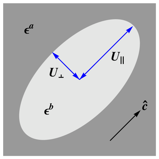
Figure 1: Schematic illustration of a spheroidal pore filled with a fluid of relative permittivity $\epsilon^{b}$, embedded in a material of relative permittivity $\epsilon^{a}$. The spheroid’s semi-major and semi-minor axes have lengths $U_{\parallel}$ and $U_{\perp}$, respectively, with the semi-major axis being aligned with the direction of $\hat{{\bf c}}$, per eqn. (2).

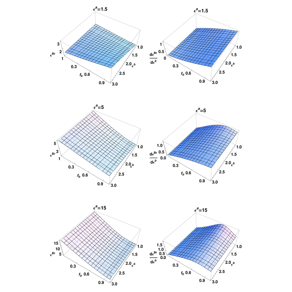
Figure 2: The Bruggeman estimate of the relative permittivity of the infiltrated porous material $\epsilon^{Br}$ plotted versus the relative permittivity of the infiltrating fluid $\epsilon^{b}\in\left(1,3\right)$ and the porosity $f_{b}\in\left(0,1\right)$, for the relative permittivity of the porous material $\epsilon^{a}\in\left\{1.5,5,15\right\}$. Also plotted are the corresponding derivatives $d\epsilon^{Br}/d\epsilon^{b}$.

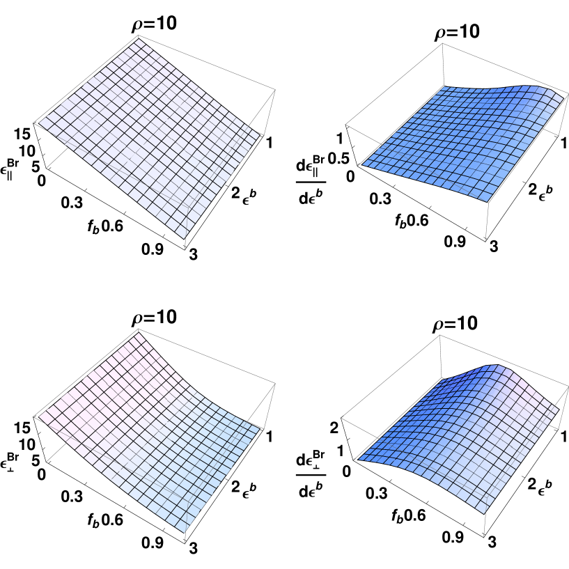
Figure 3: The Bruggeman estimate of the relative permittivity parameters of the infiltrated porous material $\epsilon^{Br}_{\perp,\parallel}$ plotted versus the relative permittivity of the infiltrating fluid $\epsilon^{b}\in\left(1,3\right)$ and the porosity $f_{b}\in\left(0,1\right)$, for the pore shape parameter $\rho=10$ and the relative permittivity of the porous material $\epsilon^{a}=15$. Also plotted are the corresponding derivatives $d\epsilon^{Br}_{\perp,\parallel}/d\epsilon^{b}$.

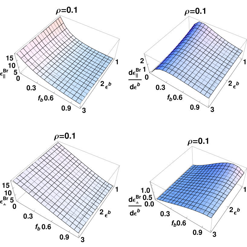
Figure 4: As Fig. 3 except that the pore shape parameter $\rho=0.1$.

References

- [1] L. De Stefano, L. Rotiroti, E. De Tommasi, I. Rea, I. Rendina, M. Canciello, G. Maglio, and R. Palumbo, “Hybrid polymer-porous silicon photonic crystals for optical sensing,” J. Appl. Phys. 106, 023109 (2009).
- [2] E. Pinet, S. Dube, M. Vachon-Savary, J.-S. Cote, and M. Poliquin, “Sensitive chemical optic sensor using birefringent porous glass for the detection of volatile organic compounds,” IEEE Sensors J. 6, 854–860 (2006).
- [3] J. J. Saarinen, S. M. Weiss, P. M. Fauchet, and J. E. Sipe, “Optical sensor based on resonant porous silicon structures,” Opt. Exp. 13, 3754–3764 (2007).
- [4] J. Homola, “Present and future of surface plasmon resonance biosensors,” Anal. Bioanal. Chem. 377, 528–539 (2003).
- [5] I. Abdulhalim, M. Zourob, and A. Lakhtakia, “Surface plasmon resonance for biosensing: A mini-review,” Electromagnetics 28, 214–242 (2008).
- [6] S. Scarano, M. Mascini, A. P. F. Turner, and M. Minunni, “Surface plasmon resonance imaging for affinity–based biosensors,” Biosens. Bioelectron. 25, 957–966 (2010).
- [7] A. Lakhtakia, R. Messier, M. J. Brett, and K. Robbie, “Sculptured thin films (STFs) for optical, chemical and biological applications,” Innovat. Mater. Res. 1, 165–176 (1996).
- [8] A. Lakhtakia, “On determining gas concentrations using thin-film helicoidal bianisotropic medium bilayers,” Sens. Actuat. B: Chem. 52, 243–250 (1998).
- [9] A. Lakhtakia, “Enhancement of optical activity of chiral sculptured thin films by suitable infiltration of void regions,” Optik 112, 145–148 (2001).
- [10] A. Lakhtakia and R. Messier, Sculptured Thin Films: Nanoengineered Morphology and Optics. Bellingham, WA, USA: SPIE Press, 2005.
- [11] R. Messier, V. C. Venugopal, and P. D. Sunal, “Origin and evolution of sculptured thin films,” J. Vac. Sci. Technol. A 18, 1538–1545 (2000).
- [12] J. A. Polo Jr, “Sculptured thin films,” in Micromanufacturing and Nanotechnology, N. P. Mahalik, Ed.. Heidelberg, Germany: Springer, 2005, pp. 357–381.
- [13] S. M. Pursel and M. W. Horn, “Prospects for nanowire sculptured-thin-film devices,” J. Vac. Sci. Technol. B 25, 2611–2615 (2007).
- [14] J. A. Polo, Jr and A. Lakhtakia, “On the surface plasmon polariton wave at the planar interface of a metal and chiral sculptured thin film,” Proc. R. Soc. A 465, 87–107 (2009).
- [15] Devender, D. P. Pulsifer, and A. Lakhtakia, “Multiple surface plasmon polariton waves,” Electron. Lett. 45, 1137–1138 (2009).
- [16] J. A. Polo, Jr, T. G. Mackay, and A. Lakhtakia, “Mapping multiple surface-plasmon-polariton-wave modes at the interface of a metal and a chiral sculptured thin film,” J. Opt. Soc. Am. B 28, 2656–2666 (2011).
- [17] T. G. Mackay and A. Lakhtakia, “Modeling chiral sculptured thin films as platforms for surface-plasmonic-polaritonic optical sensing,” IEEE Sens. J. 12, 273–280 (2012).
- [18] L. Ward, The Optical Constants of Bulk Materials and Films, 2nd ed.. Bristol, UK: Institute of Physics, 2000.
- [19] T. G. Mackay, “Effective constitutive parameters of linear nanocomposites in the long-wavelength regime,” J. Nanophoton. 5, 051001 (2011).
- [20] T. G. Mackay and A. Lakhtakia, “Determination of constitutive and morphological parameters of columnar thin films by inverse homogenization,” J. Nanophoton. 4, 041535 (2010).
- [21] T. G. Mackay and A. Lakhtakia, “Empirical model of optical sensing via spectral shift of circular Bragg phenomenon,” IEEE Photonics Journal 2, 92–101 (2010).
- [22] T. G. Mackay and A. Lakhtakia, “Modeling columnar thin films as platforms for surface–plasmonic–polaritonic optical sensing,” Photon. Nanostruct. Fundam. Appl. 8, 140–149 (2010).
- [23] W. S. Weiglhofer, A. Lakhtakia, and B. Michel, “Maxwell Garnett and Bruggeman formalisms for a particulate composite with bianisotropic host medium,” Microw. Opt. Technol. Lett. 15, 263–266 (1997). Erratum: 22, 221 (1999).
- [24] B. Michel, “A Fourier space approach to the pointwise singularity of an anisotropic dielectric medium,” Int. J. Appl. Electromagn. Mech. 8, 219–227 (1997).
- [25] B. Michel and W. S. Weiglhofer, “Pointwise singularity of dyadic Green function in a general bianisotropic medium,” Arch. Elektron. Übertrag. 51, 219–223 (1997). Erratum: 52, 31 (1998).
- [26] T. G. Mackay, A. Lakhtakia, and R. A. Depine, “Uniaxial dielectric mediums with hyperbolic dispersion relations,” Microw. Opt. Technol. Lett. 48, 363–367 (2006).
- [27] L. Bremer, R. Tuinier, and S. Jahromi, “High refractive index nanocomposite fluids for immersion lithography,” Langmuir 25, 2390–2401 (2009).
- [28] P. Schiebener and J. Straub, “Refractive index of water and steam as a function of wavelength, temperature and density,” J. Phys. Chem. Ref. Data 19, 677–717 (1990).
- [29] C. R. Simovski, “On electromagnetic characterization and homogenization of nanostructured metamaterials,” J. Optics (UK) 13, 013001 (2011).
- [30] C. Menzel, T. Paul, C. Rockstuhl, T. Pertsch, S. Tretyakov, and F. Lederer, “Validity of effective material parameters for optical fishnet metamaterials,” Phys. Rev. B 81, 035320 (2010).
- [31] J. Shin, J. T. Shen, and S. Fan, “Three-dimensional metamaterials with an ultrahigh effective refractive index over a broad bandwidth,” Phys. Rev. Lett. 102, 093903 (2009).
- [32] M. Choi, S. H. Lee, Y. Kim, S. B. Kang, J. Shin, M. H. Kwak, K.–Y. Kang, Y.–H. Lee, N. Park, and B. Min, “A terahertz metamaterial with unnaturally high refractive index,” Nature 470, 369–373 (2011).
- [33] A. Alù, M. Silveirinha, A. Salandrino, and N. Engheta, “Epsilon-near-zero metamaterials and electromagnetic sources: Tailoring the radiation phase pattern,” Phys. Rev. B 75, 155410 (2007).
- [34] G. Lovat, P. Burghignoli, F. Capolino, and D. R. Jackson, “Combinations of low/high permittivity and/or permeability substrates for highly directive planar metamaterial antennas,” IET Microw. Antennas Propagat. 1, 177–183 (2007).
- [35] M. N. Navarro-Cía, M. Beruete, I. Campillo, and M. Sorolla, “Enhanced lens by and near-zero metamaterial boosted by extraordinary optical transmission,” Phys. Rev. B 83, 115112 (2011).
- [36] J. J. H. Cook, K. L. Tsakmakidis, and O. Hess, “Ultralow-loss optical diamagnetism in silver nanoforests,” J. Opt. A: Pure Appl. Opt. 11, 114026 (2009).
- [37] T. G. Mackay, “On the effective permittivity of silver–insulator nanocomposites,” J. Nanophoton. 1, 019501 (2007).