A Simple Framework For the Dynamic Response of Cirrus Clouds to Local Diabatic Radiative Heating

ABSTRACT

This paper presents a simple analytical framework for the dynamic response of cirrus to a local radiative flux convergence, expressible in terms of three independent modes of cloud evolution. Horizontally narrow and tenuous clouds within a stable environment adjust to radiative heating by ascending gradually across isentropes while spreading sufficiently fast so as to keep isentropic surfaces nearly flat. More optically dense clouds experience very concentrated heating, and if they are also very broad, they develop a convecting mixed layer. Along isentropic spreading still occurs, but in the form of turbulent density currents rather than laminar flows. A third adjustment mode relates to evaporation, which erodes cloudy air as it lofts. The dominant mode is determined from two dimensionless numbers, whose predictive power is shown in comparisons with high resolution numerical cloud simulations. The power and simplicity of the approach hints that fast, sub-grid scale radiative-dynamic atmospheric interactions might be efficiently parameterized within slower, coarse-grid climate models.

1 Introduction

Cloud-climate feedbacks remain a primary source of uncertainty in climate forecasts (Dufresne and Bony 2008), mainly because clouds both drive and respond to the general circulation, the hydrological cycle, and the atmospheric radiation budget. Unlike fields of water vapor, clouds evolve quickly, so their radiative forcing and dynamic evolution are highly coupled on time and spatial scales that cannot be easily resolved within Global Climate Models (GCMs). For faithful reproduction of large-scale climate features, resolving radiatively driven motions on sub-grid scales may be at least as important as accurately representing mean grid-scale fluxes (Cole et al. 2005).

Radiative flux convergence and divergence within cloudy air is normally thought to produce vertical lifting and mixing motions (Danielsen 1982; Ackerman et al. 1988; Lilly 1988; Jensen et al. 1996; Dobbie and Jonas 2001). What is often overlooked is that clouds with a finite width also adjust to radiative heating by spreading horizontally, especially if the heating is concentrated in a thin layer at the cloud top or bottom (Garrett et al. 2005, 2006). Such radiatively driven mesoscale circulations have been identified within thin tropopause cirrus, and they are thought to play a role in determining the heating rate of the upper troposphere (Durran et al. 2009) and in stratospheric dehydration mechanisms (Dinh et al. 2010). Jensen et al. (2011) suggest that radiative cooling can help to initiate thin tropopause cirrus formation, while subsequent radiative heating in an environment of weak stability can induce the small-scale convection currents that are required to maintain the cloud against gravitational sedimentation and vertical wind shear.

Where these recent studies directly simulated the highly interactive and complex nature of cloud processes, an alternative and perhaps more general approach is to start with simple, analytical and highly idealized models that emphasize specific aspects of the relevant physics. Here, we look at the respose of cirrus clouds to local thermal radiative flux divergence within cloud condensate. The discussion that follows largely neglects precipitation, synoptic scale motions, and shear dynamics to facilitate description of a simple theoretical framework within a parameter space of two dimensionless numbers. A similar approach has been employed previously to constrain small-scale interactions between diabatic heating and atmospheric dynamics (Raymond and Rotunno 1989), including situations where radiation is absorbed by horizontally infinite clouds (Dobbie and Jonas 2001). Here, we extend consideration to radiatively absorptive layers that have finite lateral dimensions, an ingredient that turns out to be critical for predicting the evolution of cloud size and cross-isentropic motions. The broad intent of this study is to provide insight into how clouds respond to rapid, small-scale radiative heating in a way that might be better parameterized within large scale, coarse-grid models such as GCMs.

2 Non-equilibrium radiative-dynamic interactions in cirrus

The starting point is to consider a microphysically uniform, optically opaque cloud that is initially at rest with respect to its surrounding, characterized by a stably stratified atmosphere with a virtual potential temperature $\theta_{v}$ that increases monotonically with height (Figure 1). The arguments described below apply equally to cloud base and cloud top, differing only in sign of forcing. However, for the sake of simplicity the focus here is on cloud base.

At cloud base, cloudy air has a lower brightness temperature than the brightness temperature of the ground and lower tropospheric air that is below it. This radiative temperature difference drives a net flow of radiative energy into the colder cloud base, effectively due to a gradient in photon pressure, that can be approximated as

$$\Delta F_{net}\simeq 4\sigma\widetilde{T}_{c}^{3}\Delta\widetilde{T}$$ (1)

where $\sigma$ is the Stephan-Boltzmann constant, $\widetilde{T}_{c}$ is the cloud temperature, and $\Delta\widetilde{T}$ is the effective brightness temperature difference between the lower tropospheric air and cloud base.

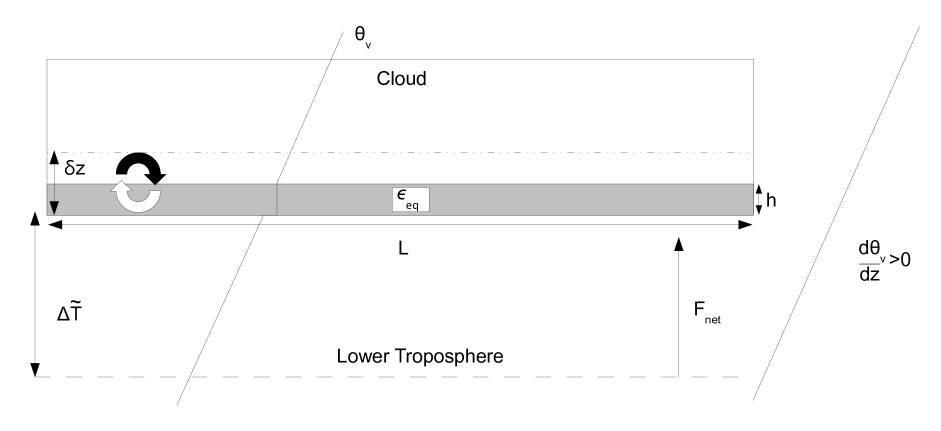
Figure 1: Radiative energy is transferred from the lower troposphere to the base of a gravitationally stratified cloud with initial width $L$, due to a radiative temperature difference $\Delta\widetilde{T}$ and deposited into a layer of characteristic depth $h$ at the base of the cloud. The layer is initially at equilibrium buoyant potential $\epsilon_{eq}$ with respect surrounding clear air at the same level, and it is perturbed from equilibrium through the deposition of radiative energy into a well-mixed layer of depth $\delta z$.

Provided the cloud is sufficiently opaque to act as a blackbody, radiative energy is deposited within a layer of characteristic depth $h$ at the base of the cloud that is smaller than the depth of the cloud itself. The magnitude of $h$ can be obtained by considering that the thermal emissivity is given by

$$\varepsilon\simeq 1-\exp(-\tau_{abs}/\bar{\mu})$$ (2)

where $\tau_{abs}$ is the absorption optical depth and $\bar{\mu}$ is the quadrature cosine for estimating the integrated contribution of isotropic radiation to vertical fluxes. Usually $\bar{\mu}\sim 0.6$ (Herman 1980). The absorption optical depth is determined by the cloud ice mixing ratio $q_{i}$, as well as the ice crystal effective radius $r_{e}$, through $\tau_{abs}=k(r_{e})q_{i}\rho\Delta z$ where $k$ is the mass specific absorption cross-section density, $\rho$ is the density of air, and $\Delta z$ is the vertical path length through which the radiation is absorbed. The depth $h$ is the e-folding path length for the attenuation such that $\tau_{abs}/\bar{\mu}=1$:

$$h=\frac{\bar{\mu}}{k(r_{e})q_{i}\rho}$$ (3)

Assuming an effective radius of 20 $\mu$m, the value for $k(r_{e})$ in cirrus is approximately 0.045 m²g^-1(Knollenberg et al. 1993). Taking, for example, $q_{i}$ values of 1 g kg^-1 that have been observed in medium sized cirrus anvils in Florida (Garrett et al. 2005), the depth $h$ would be about 30 m. As a contrasting example, a cloud with $q_{i}$ values of 0.01 g kg^-1, similar to those observed in thin cirrus (Haladay and Stephens 2009), would have a radiative penetration depth $h$ of about 3000 m. Thus, the deposition of radiative enthalpy in this layer increases its temperature at rate

$$\mathcal{H}=\frac{d\theta_{v}}{dt}=\frac{-1}{\rho c_{p}}\frac{dF}{dz}\simeq\frac{\Delta F_{net}}{\rho c_{p}h}=4\sigma\widetilde{T}_{c}^{3}\frac{k(r_{e})q_{i}}{\bar{\mu}c_{p}}\Delta\widetilde{T}$$ (4)

where $c_{p}$ is the specific heat of the air. To first order, heating rates are proportional to the radiative temperature contrast and the cloud ice mixing ratio.

a Dynamic Adjustment to Diabatic Heating

The total flow of upwelling radiative energy into a cloud is proportional to $\Delta F_{net}$ and the normal cloud horizontal cross-section, which is of order $L^{2}$ where $L$ is the cloud horizontal width. Defining the initial, neutrally buoyant, ground-state for the gravitational potential energy density of the cloudy air within the volume $hL^{2}$ as $\epsilon_{eq}=E_{eq}/\left(hL^{2}\right)$ (Figure 1), then an accumulated flow of energy into the volume increases the gravitational potential energy density to $\epsilon_{eq}+\Delta\epsilon$ at rate $d\Delta\epsilon/dt=R\Delta F_{net}/(c_{p}h)$, where $R$ is the gas constant for air. The remaining fraction ($c_{p}-R)/c_{p}=c_{v}/c_{p}$ of the radiative enthalpy deposited in the cloud goes towards increasing the rotational and translational energy density of the cloudy air within the layer. Conceptually, it is useful to consider the gravitational increase as an increase in the pressure gradient that is available to drive fluid dynamic motions: pressure gradients have units of energy density.

The increase in the potential energy density within the volume $hL^{2}$ allows work to be done against the overlying gravitational static stability to create a mixed-layer with, on average, near constant $\theta_{v}$. Thus any newly absorbed thermal energy becomes redistributed through a mixed layer depth $\delta z$ that is larger than the radiatively absorbing layer of depth $h$ (Figure 1). This is important, because it has the effect of diluting the density of newly added radiative energy through a factor of $\delta z/h$ such that:

$$\frac{d\Delta\epsilon}{dt}=\frac{R\Delta F_{net}}{c_{p}\delta z}$$ (5)

As required by the second law of thermodynamics, equilibrium is restored through relaxation of the buoyant potential energy density perturbation $\Delta\epsilon$ to zero, leading to kinematic flows (Figure 2).

Figure 2: A Schematic diagram of the thermodynamic evolution of a cirrus cloud in response to radiative diabatic heating. Potential energy flows from the warmer lower troposphere into the cooler cloud base (red arrow, left). The potential difference between the cloud and the ground is $\Delta\epsilon\simeq\frac{4}{c}\sigma T^{3}\Delta T$ where $\Delta T$ is the effective brightness temperature difference between the cloud and the lower troposphere. This flow of radiative potential energy perturbs the cloud from gravitational equilibrium at a rate $\frac{d\Delta\epsilon}{dt}$ (red arrow, right). The cloud acts to restore gravitational equilibrium at rate $\alpha\Delta\epsilon$, resulting in horizontal spreading of the cloud (blue arrows).

There are two basic modes for relaxation of the buoyant energy density. The available gravitational potential energy density $\Delta\epsilon$ can be expressed as the density $\rho$ of the air at a given buoyant potential energy density, multiplied by the buoyant potential per unit mass of air that is available to drive flows

$$\Delta E\sim N^{2}\delta z^{2}$$ (6)

Here, $N$ is the buoyancy frequency, which is related to the local stratification through

$$N^{2}=\frac{g}{\theta_{v}}\frac{d\theta_{v}}{dz}$$ (7)

It follows that

$$\Delta\epsilon=\rho N^{2}\delta z^{2}$$ (8)

Dynamic relaxation of the radiatively induced perturbation $\Delta\epsilon$ can proceed in either of two ways. At constant density, the heated volume $L^{2}\delta z$ can be raised to higher gravitational potential. Alternatively, the air expands outwards along a constant potential surface.

$$\frac{d\ln\Delta\epsilon}{dt}=\frac{\partial\ln\Delta E}{\partial t}\mid_{\rho}+\frac{\partial\ln\rho}{\partial t}\mid_{\Delta E}$$ (9)

Given Eq. 6 and that

$$\rho=\frac{m}{V}\sim\frac{m}{L^{2}\delta z}$$ (10)

where $m/\delta z$ is fixed (i.e., no entrainment of mass across the mixed-layer boundary), Eq. 9 can be rewritten as

$$\frac{d\ln\Delta\epsilon}{dt} =2\frac{\partial\ln\delta z}{\partial t}\mid_{L}-2\frac{\partial\ln L}{\partial t}\mid_{\delta z}$$ (11)

$$= \alpha_{\delta z}-\alpha_{L}$$ (12)

where $\alpha_{\delta z}$ and $\alpha_{L}$ represent instantaneous rates of adjustment.

Eq. 11 has several implications. The buoyant potential energy density $\Delta\epsilon$ within the mixed-layer volume $L^{2}\delta z$ can grow due to the continuing radiative flux deposition within the volume (the positive first term in Eq. 11). Or, it can decay through horizontal expansion (the negative second term in Eq. 11). In the first case, if the width of the cloud $L$ is held constant, the mixed-layer deepens into stratified cloudy air above it at rate

$$\frac{\partial(\delta z)}{\partial t}\mid_{L}=\frac{d\theta_{v}/dt}{d\theta_{v}/dz}=\frac{\mathcal{H}gh}{\theta_{v}N^{2}\delta z}$$ (13)

where the factor of $h/\delta z$ arises from the dilution of potential energy through a depth larger than the absorptive layer where initially, $\delta z=h$. Mixed-layer growth rates slow with time. The solution to Eq. 13 as a function of time $\Delta t$ is

$$\delta z=(\frac{\mathcal{H}gh}{\theta_{v}N^{2}}\Delta t)^{1/2}$$ (14)

Alternatively, if the depth of the mixed-layer $\delta z$ is fixed, then the potential energy density relaxes towards equilibrium by smoothing out horizontal pressure gradients between the cloudy mixed-layer and clear sky beside it. It does this through expansion of the volume $L^{2}\delta z$ along constant potential surfaces (or isentropes) into the lower potential energy density environment that surrounds the cloud. This density current outflow occurs at speed

$$u_{mix}=\frac{\partial L}{\partial t}\mid_{\delta z}\sim N\delta z$$ (15)

which results from the conversion of the gravitational potential energy of order $N^{2}\delta z^{2}$ into kinetic energy of order $u_{mix}^{2}$.

To assess the relative importance of cross-isentropic adjustment to along-isentropic spreading, a dimensionless number $S$ can be defined as the ratio of the two rates $\alpha_{\delta z}$ and $\alpha_{L}$ in Eq. 11. From Eq. 13, radiative heating increases the mixed-layer gravitational potential energy density at rate

$$\alpha_{\delta z}\sim 2\frac{\partial\ln\delta z}{\partial t}\mid_{L}=\frac{2\mathcal{H}gh}{\theta_{v}N^{2}\delta z^{2}}$$ (16)

From Eq. 15, the rate of loss of potential energy density due to expansion of the mixed-layer laterally into the clear-sky surroundings is

$$\alpha_{L}\sim 2\frac{\partial\ln L}{\partial t}\mid_{\delta z}=2\frac{N\delta z}{L}$$ (17)

For a cloud that is initially at rest, in which case a mixed layer has not yet developed, then radiation deposition remains concentrated within the layer $\delta z\sim h$ and from Eqs. 16 and 17, the ratio of these two rates can be defined by a dimensionless “Spreading Number”

$$S=\frac{\alpha_{\delta z}}{\alpha_{L}}=\frac{\partial\ln\delta z/\partial t\mid_{L}}{\partial\ln L/\partial t\mid_{\delta z}}=\frac{\mathcal{H}gL}{\theta_{v}N^{3}h^{2}}$$ (18)

If $S>1$, then the potential energy density within the layer $L^{2}\delta z$ increases due to radiative flux deposition at a rate $\alpha_{\delta z}$ that is faster than the rate $\alpha_{L}$ at which gravitational relaxation can reduce the disequilibrium in potential energy density through horizontal flows into surrounding clear air. Isentropic surfaces at cloud base cannot stay flat, but rather are deformed downward by the radiative heating. This deformation creates a deepening turbulent mixed layer that gradually grows into the overlying static stability of the atmosphere as the square root of time (Eq. 14). Meanwhile, the mixed-layer spreads outward along isentropic surfaces at rate $u_{mix}$ (Eq. 15).

By contrast, when $S<1$, adjustment through isentropic spreading is sufficiently rapid that isentropic surfaces stay approximately flat. Cloud motions stay laminar rather than becoming turbulent. The mixed-layer horizontal expansion given by $\alpha_{L}$ (Eq. 17) decreases the potential energy density faster than the rate $\alpha_{\delta z}$ (Eq. 16) at which potential energy density is deposited at cloud base through radiative flux convergence. The potential energy density at cloud base does not increase and does not overcome the overlying static stability. Rather the cloud simply lofts across isentropic surfaces at speed

$$w_{strat}=\frac{\mathcal{H}}{d\theta_{v}/dz}=\frac{\mathcal{H}g}{\theta_{v}N^{2}}$$ (19)

Dimensional continuity arguments require that the cloud spreads laterally along isentropes at speed

$$u_{strat}\sim w_{strat}\frac{L}{h}=\frac{\mathcal{H}gL}{\theta_{v}N^{2}h}$$ (20)

b Evaporative Adjustment

The above describes two modes for how radiative flux deposition can create pressure, or potential energy density gradients that drive cloud-scale motions. A third possibility for adjustment is that local radiative heating may result in microphysical changes where temperature is maintained, but condensate evaporates or condenses.

Assuming that all absorbed radiative energy goes towards evaporation at cloud base, and that there is no lag associated with the diffusion of vapor away from ice crystals, then ice evaporates at rate $\rho L_{s}dq_{i}/dt=\Delta F_{net}/h$, where $L_{s}$ is the latent heat of sublimation. Substituting Eq. 3 for $h$, radiative heating evaporates cloud base at rate

$$\alpha_{evap}=\left|\frac{d\ln q_{i}}{dt}\mid_{T}\right|=\frac{k(r_{e})\left|\Delta F_{net}\right|}{\bar{\mu}L_{s}}$$ (21)

Note that if there were net radiative flux divergence, as might be expected at the top of a thermally opaque cloud, then net cooling would lead to condensation.

The ratio of $\alpha_{evap}$ (Eq. 21) to $\alpha_{\delta z}$ (Eq. 16) implies a dimensionless “Evaporation Number” comparing the evaporation rate to the rate of laminar adjustment through cross isentropic ascent. In the initial stages of development, where $\delta z=h$,

$$E=\frac{\alpha_{evap}}{\alpha_{\delta z}}=\frac{\theta_{v}N^{2}h}{2g\mathcal{H}}\frac{k(r_{e})\left|\Delta F_{net}\right|}{\bar{\mu}L_{s}}$$ (22)

or, substituting Eq. 7 and Eq. 4 for the heating rate $\mathcal{H}$

$$E=\frac{c_{p}h}{L_{s}q_{i}}\frac{d\theta_{v}}{dz}$$ (23)

The susceptibility to evaporation depends only on the cloud microphysics and the local static stability, and not, in fact, on the magnitude of the heating. Provided $E>1$, cloud base evaporates rather than lofts. However, for values of $E<1$, cloud ascends faster than it evaporates and condensate is maintained. It is important to note here that the “Evaporation Number” $E$ should only be considered if the “Spreading Number” $S$ has values smaller than unity. If $S>1$, the relevance of evaporation is less clear because a convective mixed-layer develops, in which case one would expect instead continual reformation and evaporation of cloud condensate as part of localized circulations within the mixed-layer. The more relevant comparison might be to rates of turbulent entrainment and mixing.

3 Numerical Model

To test the suitability of the dimensionless “Spreading” and “Evaporation” numbers $S$ and $E$ for determining the cloud evolutionary response to local diabatic heating, we made comparisons to cloud simulations from the University of Utah Large Eddy Simulation Model (UU LESM) (Zulauf 2001). An LES model is used because the resolved scales are sufficiently small to represent turbulent motions, convection, entrainment and mixing, and laminar flows.

The UU LESM is based on a set of fully prognostic 3D non-hydrostatic primitive equations that use the quasi-compressible approximation (Zulauf 2001). The model domain was placed at the equator, $\phi=0^{\circ}$, to eliminate any Coriolis effects. Even in the largest domain simulations, the maximum departure from the equator (50 km) is sufficiently small as to justify not including the Coriolis effect in the model calculations.

The horizontal extent of the domain was chosen to contain the initialized cloud as well as to allow sufficient space for spreading of the cloud during the model run. The UU LESM model employs periodic boundary conditions such that fluxes through one side of the domain (moisture, cloud ice, turbulent fluxes, etc.) enter back into the model domain from the opposite side. Here, the horizontal domain size is case dependent but chosen to be sufficiently large as to minimize “wrap around” effects. Horizontal grid size was chosen to be 30 m to match the minimum value for vertical penetration depth of radiation into the cloud, but it increased to 100 m for cases that required particularly large and computationally expensive domains.

The vertical domain spanned 17 km and included a stretched grid spacing. The highest resolution for the stretched grid was placed at the center of the initial cloud with grid size of 30 m. The vertical resolution decreased logarithmically to a maximum grid spacing of approximately 300 m at the top of the model and approximately 400 m at the surface. A sponge layer was placed above 14 km to dampen vertical motions at the top of the model and to prevent reflection of gravity waves off the top of the model domain. The model time step for dynamics was between 1.0 and 10.0 s and was chosen to be the largest time step that was computationally stable.

For radiative transfer, the UU LESM model uses a plane parallel broadband approach, using a $\delta$-four stream scheme for parameterization of radiative transfer (Liou et al. 1988), based on the correlated k-distribution method (Fu and Liou 1992). Radiative transfer calculations were performed at a time step of 60 s. Only thermal radiation was considered in this study.

For all cases examined, the model was initialized with a standard tropical profile of temperature and atmospheric gases with a buoyancy frequency $N$ of approximately 0.01 s${}^{\text{-1}}$ throughout the depth of the model domain. Relative humidity was set in two independent layers. In the bottom layer of the model, which extends from the surface to 7.8 km, the relative humidity was set to a constant 70% with respect to liquid water. In the upper layer of the model, from 7.8 km upwards, which contained the cloud between 8.8 km and 11.3 km, relative humidity with respect to ice was set to a constant value of 70%. All clouds were initialized as homogeneous cylindrical ice clouds, as shown in Figure 3. Ice particles within the cloud were of uniform size with a fixed effective radius of 20 $\mu$m and an initially uniform mixing ratio as prescribed by the particular case. Cloud radius was prescribed according to the particular case, but in each case the thickness was set to 2500 m with the cloud base set at 8.8 km. Cloud base was chosen such that the cloud top would be placed at approximately 200 mb, in rough accordance with the average cirrus anvil height indicated by the Fixed Anvil Temperature hypothesis (Hartmann and Larson 2002). Both the cloud and surrounding atmosphere were initialized to be at rest. No precipitation was allowed in any of the model simulations. Cloud particle fall speed was also neglected. All cases were run for one hour of model simulation time.

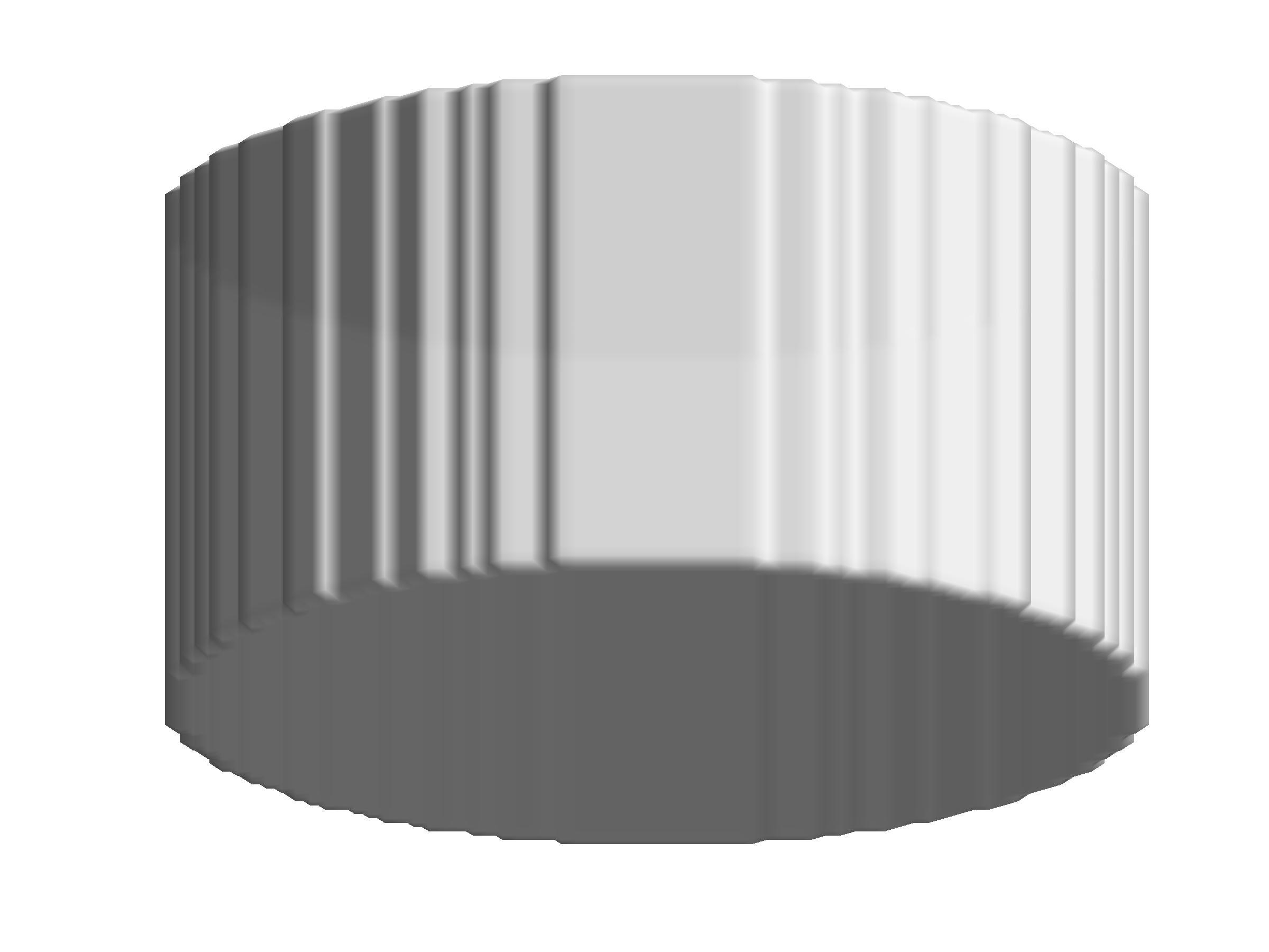
Figure 3: 3D surface of cloud as initialized for all simulations

Two cloud parameters were varied through several orders of magnitude in order to explore a wide parameter space of possible evolutionary behaviors. Cloud radius $L$ was chosen to be 100 m, 1 km, or 10 km. The ice-water mixing ratio $q_{i}$ was set to 0.01, 0.1, or 1 g kg^-1. This provided 9 unique combinations of cloud size and density, as described in Tables 1 and 2, that spanned a range of values of $S$ and $E$, and included combinations that are sufficiently unstable that they are not observed naturally.

Table 1: Spreading number $S=\frac{\alpha_{\delta z}}{\alpha_{L}}=\frac{\mathcal{H}gL}{\theta N^{3}h^{2}}$

	$L$=100m	1km	10km
$q_{i}$=0.01g/kg	1.1$\times$10-4	1.1$\times$10-3	0.011
0.1g/kg	3.3$\times$10-3	0.033	0.33
1g/kg	13	130	1300

Table 2: Evaporation number $E=\frac{\alpha_{evap}}{\alpha_{\delta z}}=\frac{c_{p}\theta N^{2}h}{gL_{s}q_{i}}$

	$L$=100m	1km	10km
$q_{i}$=0.01g/kg	150	150	150
0.1g/kg	3.7	3.7	3.7
1g/kg	0.037	0.037	0.037

Figure 4 shows the initial heating rate profiles for each value of $q_{i}$ used in this study calculated using the Fu and Liou (1992) radiative transfer parameterization. Note that the heating is confined to a narrower layer at cloud base as the ice water mixing ratio increases (Eq. 3). The heating profiles for both the $q_{i}=0.01$ g kg^-1 and $q_{i}=0.1$ g kg^-1 cases closely match the calculated heating rate profiles from Lilly (1988). However, the heating rate profile for the $q_{i}=1$ g kg^-1 case, which Lilly did not model, shows an order of magnitude increase in the heating and cooling rates to several hundred K day^-1, confined almost exclusively to the top and bottom of the cloud, with virtually no heating in the interior.

For cases with $q_{i}=0.01$ g kg^-1, the radiative penetration depth $h$ is 3300 m, which is deeper then the 2500 m cloud depth. However, the heating profile is nearly linear through the depth of the cloud with heating at cloud base and cooling at cloud top. Thus, in cases where $q_{i}$ is 0.01 g kg^-1, the radiative penetration depth $h$ is assumed to be half the cloud depth, or 1250 m, for the purposes of calculating $S$ and $E$.

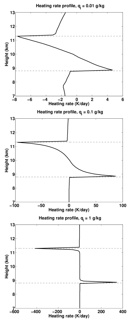
Figure 4: Heating rate profiles for $q_{i}=0.01$ g kg^-1, $q_{i}=0.1$ g kg^-1, and $q_{i}=1$ g kg^-1. Cloud vertical boundaries are marked with a dashed line.

4 Results

In the parameter space of $S$ and $E$ described by Tables 1 and 2, tenuous and narrow clouds with low values of ice water mixing ratio $q_{i}$ and cloud width $L$ have values of the spreading number $S$ that are less than 1. Theoretically, such clouds are expected to undergo laminar lifting and spreading. Tenuous clouds with large values of $E$ and small value of $S$ are expected to evaporate at cloud base. Optically dense and broad clouds with large values of $q_{i}$ and $L$ have values of $S$ much larger than 1, and are expected to favor the concentration of potential energy density in a thin layer at cloud base, leading to turbulent mixing and erosion of stratified air within the cloudy interior.

In what follows, numerical simulations are performed to test the validity of the dimensionless numbers $S$ and $E$ for predicting cloud evolution. Cases that describe the parameter space in $S$ will be discussed first, since values of $E$ are relevant only for scenarios with $S<1$ where mixed-layer development is not the primary response to local diabatic radiative heating.

a Isentropic Adjustment

Simulations of clouds with values of $S<1$ are expected to show cross-isentropic ascent of cloud base in response to local diabatic radiative heating and, through continuity, laminar spreading. Effectively, the loss of potential energy out the sides of the cloud (due to material flows) is sufficiently rapid to maintain nearly flat isentropic surfaces within the original cloud volume. Equivalently, cross-isentropic ascent is sufficiently slow that the consequent horizontal pressure gradients can be equilibrated through laminar spreading while keeping isentropic surfaces approximately flat (Eq. 17).

A good example of this behavior is shown in a simulation of a cloud with $L=1$ km and $q_{i}=0.1$ g kg^-1. This case has a value of $S=0.033$, which implies that the primary response to radiative heating should be adjustment through ascent across isentropic surfaces. Figure 5 shows the isentropes, or contours in $\theta_{e}$. The isentropes remain approximately flat and unchanged from their initial state in response to the cross-isentropic flow of cloudy air. As shown in Figure 6, the simulated cloud undergoes rising at cloud base and sinking at cloud top, while spreading horizontally.

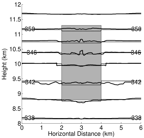
Figure 5: Cross section of $\theta_{e}$ contours through a cloud with $L$=1km and $q_{i}$=0.1 g kg^-1 ($S=0.033$) after 0 s (thin) and 3600 s (thick) of simulation. The initial cloud boundaries are indicated by the shaded region.

Figure 6: as in Figure 5, but a 3D surface plot of $q_{i}$ after 3600 s of simulation (top), and a plot of a $q_{i}$ cross section of the cloud (bottom). The initial position of the cloud is shown in black, while the state of the cloud after 3600 s is shown in color, with the value of $q_{i}$ denoted by the color scale. Note the rise of cloud base and the horizontal spreading.

b Mixing

Clouds with values of $S>1$ are not expected to be associated with laminar motions. Instead, radiative heating bends down isentropic surfaces so rapidly as to create a local instability that cannot be restored sufficiently rapidly by laminar cloud outflows (Eq. 16). Radiative heating is sufficiently concentrated to initiate turbulent mixing that produces a growing mixed-layer. Unlike the $S<1$ case, isentropes do not stay flat.

An example, shown in Figure 7, is for a simulated cloud that has initial condition values of cloud radius $L=10$ km and ice water mixing ratio $q_{i}=1$ g kg^-1. Since $S=1300$, it is expected that the potential energy density at cloud base will increase at a rate that is faster than the loss rate of potential energy through cloud lateral expansion (Eqs. 16 and 17). A mixed layer will develop because the deposition of radiative energy creates buoyancy that does work to overcome the static stability of overlying cloudy air and create a mixed layer. Meanwhile the mixed-layer expands with speed $u_{mix}=N\delta z$ (Eq. 15), where $\delta z$ is the mixed-layer depth and $N$ is the static stability of air surrounding the cloud.

The numerical simulations reproduce these features. A mixed-layer can be seen in the $\theta_{v}$ profile plotted in Figure 7, showing the average cloud properties after 1 hour of model simulation. This profile is a horizontally averaged profile taken within 9 km of cloud center. On average, the mixed-layer exhibits a nearly adiabatic profile in $\theta_{v}$. At 1 h simulation time, the mixed-layer at cloud base is nearly 800 m deep. The mixed layer expands horizontally along isentropes, as seen in Figure 8. The “bowl” shaped spreading of the cloud is because intense radiative heating at cloud base bends isentropic surfaces downward.

Figure 7: $\theta_{v}$ profile of a cloud with $L$=10 km and $q_{i}$=1 g kg^-1 after 3600 s of simulation. The initial profile is plotted in a dashed line with horizontal dashed lines indicating initial cloud base and cloud top. The $\theta_{v}$ profile is calculated as a horizontal average of all $\theta_{v}$ profiles within an annular region of the cloud. The inner edge of the annulus is 7.5 km from cloud center and the outer edge of the annulus is at 9 km from cloud center.

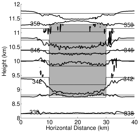
Figure 8: As in Figure 7 but a cross section of $\theta_{e}$ contours through a cloud after 0 s (thin) and 3600 s (thick) of simulation. The initial cloud boundaries are indicated by the shaded region.

This mixed-layer development and spreading can also be seen in cross sectional plots of $q_{i}$ in Figure 9. There is a mixed-layer at both cloud base and cloud top with darker shading indicating where drier air has been entrained from below or above. Note that cloud base and cloud top remain at roughly constant elevation. In Figure 5, for a case where $S\ll 1$, radiative flux convergence at cloud base drives cross-isentropic laminar ascent. In this case, where $S\gg 1$, laminar ascent does not occur. Instead, cloud base remains nearly at its initial vertical level and there is formation of a turbulent mixed layer that spreads outward along isentropes. Notably, the mixed-layer circulations at cloud base have a mammatus-like quality to them, something we have discussed more extensively in Garrett et al. (2010).

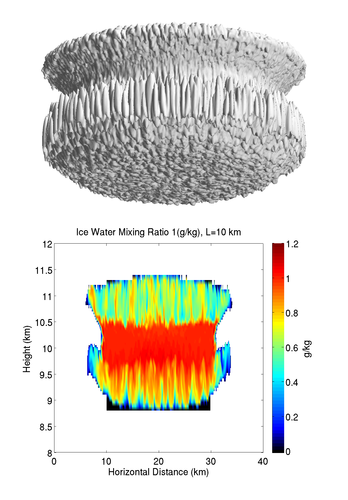
Figure 9: As in Figure 7, but a 3D surface plot of $q_{i}$ after 3600 s of simulation (top), and a plot of a $q_{i}$ cross section of the cloud (bottom). The initial position of the cloud is shown in black, while the state of the cloud after 3600 s is shown in color, with the value of $q_{i}$ denoted by the color scale. Note that cloud base remains at roughly the same level and that the cloud bends upward as it spreads outward.

These behaviors can be quantified by examination of the rapidity of development of a well-mixed layer at cloud base. If the dominant mode of evolution is cross-isentropic lofting, then vertical potential temperature gradients should remain relatively undisturbed. Conversely, if mixing is the dominant response, then potential temperature will evolve to become more constant with height.

Table 3 shows the cloud domain-averaged, logarithmic rate of decrease in the static stability $d\ln N^{2}/dt$, where $N^{2}\propto d\theta_{v}/dz$. Calculations are evaluated for the lowermost 80 m of the cloud within the initial 360 s of simulation time. The destabilization of cloud base reflects the magnitude of the Spreading Number $S$ (Table 1), with large values of $S$ demonstrating the most rapid rates of mixed-layer development.

Table 3: Rate of destabilization at cloud base ($-d\ln N^{2}/dt$) in units of hr^-1. Cases with a Spreading Number $S$ that is much greater than one are indicated in bold.

	$L$=100m	1km	10km
$q_{i}$=0.01g/kg	0.12	0.17	0.15
0.1g/kg	1.32	0.83	1.94
1g/kg	4.00	11.42	23.88

c Evaporation

Cloud bases with $S<1$ and $E>1$ are expected to evaporate more quickly than they loft across isentropes (Table 2). For example, for a cloud with $L=1$ km and $q_{i}=0.01$ g kg^-1 , the calculated value of the Spreading Number $S$ is 0.0011, and the value of the Evaporation number $E$ is 150. Based on these values, the expected evolution of cloud base would be gradual evaporative erosion of cloud base.

To quantify the importance of evaporation to cloud evolution, the rate of change in cloud mass $d\ln m/dt$, where $m$ is the mass of cloud ice, was calculated over the first 180 s of simulation, but only within the lower layer in which radiation from the surface is absorbed, $h$, rather than the entire cloud. The absorptive layers were taken to be 30 m, 300 m, and 1250 m for cloud ice water mixing ratios of 1 g kg^-1, 0.1 g kg^-1, and 0.01 g kg^-1 respectively.

Table 4: Evaporation rate, in units of h^-1, defined here as the negative of the logarithmic rate of mass change in the lower depth $h$ of the cloud nto the cloud within the initial 180 s of simulation in units of s for cases where $E>1$ and $S<1$

	$E$ = 150	$E$ = 3.7
$L$ = 100 m	5.8	0.79
1 km	4.0	0.72
10 km	1.5	0.68

From Eq. 21 for $\alpha_{evap}$, the anticipated evaporation rate at cloud base is approximately $7$ h^-1 based on the modeled net flux absorption $\Delta F$ of 74 $W$ m^-2 within the absorption layer $h$. Table 4 shows maximum modeled evaporation rates that are nearly as large, at least where $E$ is maximized and the cloud is narrow. However, rates of evaporation decrease with increasing cloud width $L$, perhaps because $S$ increases and stronger dynamic motions at cloud base replace evaporated cloud condensate with newly formed cloud matter. In general, however, tenuous cirrus clouds are most susceptible to erosion by evaporation at cloud base, particularly if they are not very broad.

d Precipitation

While the role of precipitation has been excluded from these simulations in order to clarify the physical behavior, certainly natural clouds can have significant precipitation rates. An estimate of the relative importance of precipitation is briefly discussed here.

The characteristic precipitation timescale $\alpha_{precip}$ depends on the rate of depletion of cloud water by precipitation $P$ and the average ice water content $IWC$. For example, in a cirrus anvil in Florida measured by aircraft during the CRYSTAL-FACE field campaign, the measured value of $P$ was 0.05 g m^-3 h^-1 compared to values of $IWC$ of 0.3 g m^-3 (Garrett et al. 2005), implying a precipitation depletion rate $\alpha_{precip}=P/IWC=0.15$ h^-1. For comparison, corresponding values for the radiative adjustment rates are $\alpha_{L}\simeq 0.11$ h^-1 (Eq. 17) and $\alpha_{\delta z}\simeq 144$ h^-1 (Eq. 16). While development of a turbulent mixed layer is the fastest process, precipitation depletes cloud condensate at a rate that is comparable to $\alpha_{L}$, the rate at which gravitational equilibrium is restored through cross-isentropic flows and laminar spreading.

5 Discussion

We have separated the evolutionary response of clouds to local diabatic heating into distinct modes of cross-isentropic lifting, along-isentropic spreading, and evaporation of cloud condensate. A straightforward method has been described for determining how a cloud will evolve based on ratios of the associated rates. The dominant modes of evolution are outlined in Table 5.

Table 5: Dominant modes of evolution observed in simulations. Cases where the Spreading Number $S$ and Evaporation Number $E$ are much greater than one are indicated in bold and italics, respectively.

	$L$=100m	1km	10km
$q_{i}$=0.01g/kg	evaporation	evaporation	evaporation
0.1g/kg	lofting	lofting	mixing
1g/kg	mixing	mixing	mixing

For example, cirrus anvils begin their life cycle as dense cloud from convective towers that have reached their level of neutral buoyancy (Scorer 1963; Jones et al. 1986; Toon et al. 2010). Such broad optically thick clouds are associated with high values of the spreading number $S$ due to their large horizontal extent and high concentrations of cloud ice. Radiative flux convergence is confined to a thin layer at cloud base. Heating is so intense, and the cloud is so broad, that the cloudy heated air cannot easily escape by spreading into surrounding clear air. Instead, large values of $S$ favor the development of a deepening mixed-layer. The mixed-layer still spreads, but in the form of turbulent density currents rather than laminar motions.

However, as the cloud spreads and thins, the value of the spreading number $S$ evolves. $S$ is proportional to the heating rate $\mathcal{H}$, cloud width $L$, and inversely proportional to the square of the depth of the mixed layer $\delta z^{2}$ (Eq. 18). Cloud spreading increases the value of $L$, and this acts as a positive feedback on $S$. But as the cloud spreads, the mixed-layer depth increases as $t^{1/2}$ (Eq. 14), progressively diluting the impact of radiative heating on dynamic development by a factor of $\delta z/h$. Thus, while cloud spreading increases $S$, this is offset by increasingly diluted heating rates within the mixed-layer (Eq. 18).

From Eq. 18, $S$ can be rewritten as

$$S=A\frac{L}{\delta z^{3}}$$ (24)

where $A=\mathcal{H}gh/\theta_{v}N^{3}$ is assumed to be constant, assuming here that $q_{i}$ is fixed. Thus, the rate of change in $S$ is given by

$$\frac{d\ln S}{dt}\mid_{q_{i}}=\frac{d\ln L}{dt}-3\frac{d\ln\delta z}{dt}$$ (25)

From Eq. 13, and since $dL/dt=u_{mix}\sim N\delta z$ (Eq. 15), Eq. 25 can be rewritten as

$$\frac{d\ln S}{dt}\mid_{q_{i}}=\frac{N\delta z}{L_{0}}-\frac{3NA}{\delta z^{2}}$$ (26)

Finally, from Eq. 14, if the mixed layer depth evolves over time as $\delta z=(NAt)^{1/2}$, Eq. 26 becomes

$$\frac{d\ln S}{dt}=\frac{(N^{3}At)^{1/2}}{L_{0}}-\frac{3}{t}$$ (27)

Thus, the evolution of $S$ is controlled by two terms, the first being a positive feedback related to cloud spreading, and the second being a negative feedback related to mixed-layer deepening. Provided that

$$t<t_{max}=\left(\frac{9L_{o}^{2}}{AN^{3}}\right)^{1/3}$$ (28)

the negative feedback dominates, so that to a good approximation

$$\frac{d\ln S}{d\ln t}\simeq-3$$ (29)

which can be solved for the general solution

$$S(t)\simeq S_{o}\left(\frac{t_{0}}{t}\right)^{3}$$ (30)

For a thick cirrus anvil with initial values of $q_{i}$ of 1 g kg^-1, $L$ of 10 km, and $S$ of 1300, the value of $A$ is 3510 m² and $t_{max}\simeq 10$ h. By comparison, from Eq. 30, the value of $S$ rapidly drops to a value of approximately unity within time $t\simeq 10t_{0}$. While the value of $t_{0}$ is not explicitly defined, assuming that it is one buoyancy period $2\pi/N$, then the time scale for the cirrus anvil to shift from turbulent mixing to isentropic adjustment is of order one hour. Because this timescale is much less than $t_{max}$, the anvil never manages to enter a regime of runaway mixed-layer deepening where Eq. 27 is positive. What is interesting is that this timescale for a convecting anvil to move into a laminar flow regime is comparable to the few hours lifetime of tropical cirrus associated with deep-convective cloud systems (Mace et al. 2006). A transition to laminar behavior seems inevitable.

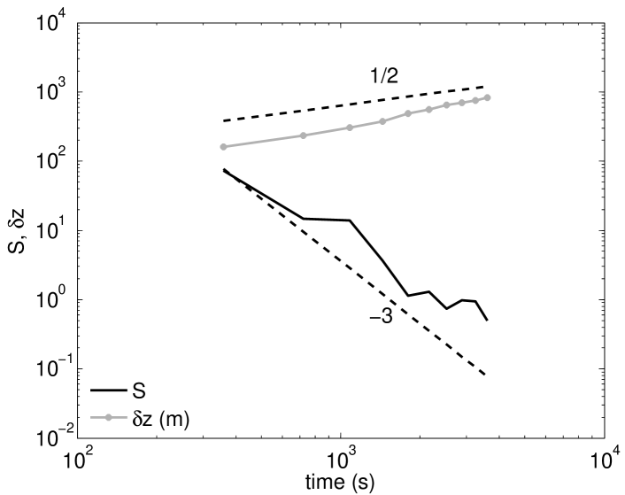
Figure 10: The time evolution of the Spreading Number $S$ and the mixed-layer depth $\delta z$ of a cloud with ice water mixint ratio $q_{i}$ of 1 g kg^-1 and width $L$ of 10 km from 0 to 3600 s. The dashed lines indicates slopes of 1/2 and -3 on the log-log plot as indicated.

Figure 10 shows numerical simulations for the time evolution of $S$ within the cloud base domain. These reproduce the theoretically anticipated decay at a rate close to the anticipated $t^{-3}$ power law. The decay in $S$ is dominated by mixed-layer deepening, which roughly follows the anticipated $t^{1/2}$ power law. It may seem counter-intuitive, but it is deepening of a turbulent mixed-layer that allows for a transition to laminar behavior: current radiative flux deposition becomes increasingly diluted in past deposition. Once an anvil reaches $S\sim 1$, the rate at which the mixed layer deepens becomes roughly equal to the rate at which laminar flow restores gravitational equilibrium through spreading. At this point, the dynamic evolution of the cirrus anvil enters a new regime where it adjusts to any radiatively induced gravitational disequilibrium through either cross-isentropic lofting (Danielsen 1982; Ackerman et al. 1988) or evaporation (Jensen et al. 1996).

As a contrasting example, contrail formations are typically optically thin and horizontally narrow. In some cases they can evolve into broad swaths of cirrus that persist for up to 17 hours after initial formation and radiatively warm the surface (Burkhardt and K rcher 2011). While we did not specifically model contrails in this study, the theoretical principles that we discussed can provide guidance for how they might be expected to evolve.

Immediately following ejection from a jet engine, the contrail air has water contents of a few tenths of a gram per meter cubed (Spinhirne et al. 1998), contained within a very narrow horizontal domain (Voigt et al. 2010). In this case, the cloud can be characterized in an idealized sense by $q_{i}=$1 g kg^-1 and $L=$100 m (Table 1). Since the expressions for $A$ and $t_{max}$ discussed above do not depend on the horizontal extent of the cloud $L$, their values are identical to those of the idealized anvil that was explored. However, the initial value of $S$ does depend on $L$, and with an initial value of 13 it is one hundred times smaller than for the anvil case. Since the initial value for $S$ is still larger than unity, it should be expected that the contrail cirrus will be able to sustain radiatively driven turbulent mixing in its initial stages. However, from Eq. 30, $S$ should be expected to decline to unity in about 20 minutes, at which point more laminar circulations take over that allow for the contrail cloud to spread laterally while slowly lofting across isentropes.

6 Conclusions

In this study, the evolutionary behavior of idealized clouds in response to local diabatic heating was estimated from simple theoretical arguments and then compared to high resolution numerical simulations. Simulated clouds were found to evolve in a manner that was consistent with expected behaviors. Dense, broad clouds had high initial values of a spreading number $S$ (Eq. 18) and formed deepening convective mixed-layers at cloud base that spread in turbulent density currents. The mixed-layers were created because isentropic surfaces were bent downward by radiative flux convergence to create a layer of instability. The mixed-layer deepened at a rate $\alpha_{\delta z}$ (Eq. 16) that was much faster than the rate at which the potential instability could be restored through along-isentropic outflow into surrounding clear air at rate $\alpha_{L}$ (Eq. 17). For particularly high values of $S$, the mixed-layer production from radiative heating was so strong as to create mammatus clouds at cloud base (Garrett et al. 2010).

Tenuous and narrow clouds with initial values of $S<1$ displayed gradual laminar ascent of cloud base across isentropic surfaces while the cloud spread through continuity into surrounding clear sky. Isentropic surfaces stayed roughly flat because the rate of along-isentropic spreading $\alpha_{L}$ (Eq. 17) was sufficiently rapid compared to the rate of cross-isentropic lifting $\alpha_{\delta z}$ (Eq. 16) that isentropic surfaces in the cloud were continuously returned to their original equilibrium heights. Clouds with low values of $S$ and also high values of an evaporation number $E$ (Eq. 23) tended to evaporate quickly because the rate at which cloud condensate evaporated $\alpha_{evap}$ (Eq. 21) was much faster than the rate at which the cloud layer rose in cross-isentropic laminar ascent $\alpha_{L}$ (Eq. 17).

For clouds with values of $S$ that are initially high, the tendency is that $S$ falls with time as the convergence of radiative flows at cloud base becomes increasingly diluted in a deepening mixed-layer. We found that dense cirrus anvils with a large horizontal extent remain in a mixed-layer deepening regime for nearly an hour before shifting across the $S=1$ threshold into a cross-isentropic laminar lofting regime. Contrail cirrus are expected to make the same transition, but in a matter of tens of minutes.

It is important to note that the precision of any of these results is limited by the simplifications that were taken. Most important is that no precipitation was included in the numerical simulations, so simulated clouds presumably persisted longer than if precipitation were included. Also, single-sized ice particles were used rather than a distribution of ice particle sizes. Gravitational sorting would result in a higher concentration of larger ice particles near cloud base and a higher concentration of small ice particles near cloud top (Garrett et al. 2005; Jensen et al. 2010).

Nonetheless, it has been shown that local diabatic heating heating can drive dynamic motions and microphysical changes that are at least as important as precipitation, and easily predicted from the simple calculation of two dimensionless numbers. A practical future application of this work might be improved constraints of the fast, smale-scale evolution of fractional cloud coverage within a GCM gridbox, limiting the need for explicit, and expensive, fluid simulations of sub-grid scale processes.

REFERENCES

- Ackerman et al. (1988) Ackerman, T. P., K. N. Liou, F. P. J. Valero, and L. Pfister, 1988: Heating rates in tropical anvils. J. Atmos. Sci., 45, 1606–1623.
- Burkhardt and K rcher (2011) Burkhardt, U. and B. K rcher, 2011: Global radiative forcing from contrail cirrus. Nature Climate Change, 1, 54–58, doi:10.1038/nclimate1068.
- Cole et al. (2005) Cole, J. N. S., H. W. Barker, D. A. Randall, M. F. Khairoutdinov, and E. E. Clothiaux, 2005: Global consequences of interactions between clouds and radiation at scales unresolved by global climate models. Geophys. Res. Lett., 32, L06 703, doi:10.1029/2004GL020 945.
- Danielsen (1982) Danielsen, E. F., 1982: A dehydration mechanism for the stratosphere. Geophys. Res. Lett., 9, 605–608.
- Dinh et al. (2010) Dinh, T. P., D. R. Durran, and T. Ackermann, 2010: The maintenance of tropical tropopause layer cirrus. J. Geophys. Res., 115, D02 104, doi:10.1029/2009/JD012 735.
- Dobbie and Jonas (2001) Dobbie, S. and P. Jonas, 2001: Radiative influences on the structure and lifetime of cirrus clouds. Q.J.R.Meteorol.Soc., 127, 2663–2682, doi:10.1002/qj.49712757 808.
- Dufresne and Bony (2008) Dufresne, J. L. and S. Bony, 2008: An assessment of the primary sources of spread of global warming estimates from coupled ocean-atmosphere models. J. Climate, 21, 5135–5144, doi:10.1175/2008JCLI2239.1.
- Durran et al. (2009) Durran, D. R., T. Dinh, M. Ammerman, and T. Ackerman, 2009: The mesoscale dynamics of thin tropical tropopause cirrus. J. Atmos. Sci, 66, 2859–2873, doi:10.1175/2009JAS3046.1.
- Fu and Liou (1992) Fu, Q. and K. N. Liou, 1992: On the correlated k-distibution method for radiative transfer in nonhomogeneous atmospheres. J. Atmos. Sci., 49, 2139–2156.
- Garrett et al. (2010) Garrett, T. J., C. T. Schmidt, S. Kihlgren, and C. Cornet, 2010: Mammatus clouds as a response to cloud-base radiative heating. J. Atmos. Sci., 67, 3891–3903, doi:10.1175/2010JAS3513.1.
- Garrett et al. (2006) Garrett, T. J., M. A. Zulauf, and S. K. Krueger, 2006: Effects of cirrus near the tropopause on anvil cirrus dynamics. Geophysical Research Letters, 33.
- Garrett et al. (2005) Garrett, T. J., et al., 2005: Evolution of a Florida cirrus anvil. J. Atmos. Sci., 62, 2352–2371, doi:10.1175/JAS3495.1.
- Haladay and Stephens (2009) Haladay, T. and G. Stephens, 2009: Characteristics of tropical thin cirrus clouds deduced from joint CloudSat and CALIPSO observations. J. Geophys. Res., 114, D00A25, doi:10.1029/2008JD010 675.
- Hartmann and Larson (2002) Hartmann, D. L. and K. Larson, 2002: An important constraint on tropical cloud-climate feedback. Geophysical Research Letters, 29, 1951–1955, doi:10.1029/2002GL015 835.
- Herman (1980) Herman, G. F., 1980: Thermal radiation in arctic stratus clouds. Quart. J. Roy. Meteor. Soc., 106, 771–780.
- Jensen et al. (2010) Jensen, E. J., L. Pfister, T. P. Bui, P. Lawson, and D. Baumgardner, 2010: Ice nucleation and cloud microphysical properties in tropical tropopause layer cirrus. Atmos. Chem. Phys., 10, 1369–1384, doi:10.5194/acp–10–1369–2010.
- Jensen et al. (2011) Jensen, E. J., L. Pfister, and O. B. Toon, 2011: Impact of radiative heating, wind shear, temperature variability, and microphysical processes on the structure and evolution of thin cirrus in the tropical tropopause layer. J. Geophys. Res., 116, D12 209, doi:10.1029/2010JD015 417.
- Jensen et al. (1996) Jensen, E. J., O. B. Toon, H. B. Selkirk, J. D. Spinhirne, and M. R. Schoeberl, 1996: On the formation and persistence of subvisible cirrus clouds near the tropical tropopause. J. Geophysical Research, 101, 21,361–21,375.
- Jones et al. (1986) Jones, R. L., J. A. Pyle, J. E. Harries, A. M. Zavody, J. M. R. III, and J. C. Gille, 1986: The water vapour budget of the stratosphere studied using LIMS and SAMS satellite data. Quart. J. Roy. Meteor. Soc., 112, 1127–1143.
- Knollenberg et al. (1993) Knollenberg, R. G., K. Kelly, and J. C. Wilson, 1993: Measurements of high number densitied of ice crystals in the tops of tropical cumulonumbus. J. Geophys. Res., 98, 8639–8664.
- Lilly (1988) Lilly, D. K., 1988: Cirrus outflow dynamics. J. Atmos. Sci., 45, 1594–1605.
- Liou et al. (1988) Liou, K. N., Q. Fu, and T. P. Ackerman, 1988: A simple formulation of the delta-four-stream approximation for radiative transfer parameterizations. J. Atmos. Sci., 45, 1940–1947.
- Mace et al. (2006) Mace, G. G., M. Deng, B. Soden, and E. Zipser, 2006: Association of tropical cirrus in the 10-15-km layer with deep convective sources: An observational study combining millimiter radar data and satellite-derived trajectories. J. Atmos. Sci, 63, 480–503, doi:10.1175/JAS3627.1.
- Raymond and Rotunno (1989) Raymond, D. J. and R. Rotunno, 1989: Response of a stably stratified flow to cooling. J. Atmos. Sci., 46, 2830–2837.
- Scorer (1963) Scorer, R. S., 1963: Cloud nomenclature. Quart. J. Roy. Meteor. Soc., 89, 248–253.
- Spinhirne et al. (1998) Spinhirne, J. D., W. D. Hart, and D. P. Duda, 1998: Evolution of the morphology and microphysics of contrail cirrus from airborne remote sensing. Geophys. Res. Lett., 25, 1153–1156, doi:10.1029/97GL03 477.
- Toon et al. (2010) Toon, O. B., et al., 2010: Planning, implementation, and first results of the tropical composition, cloud and climate coupling experiment (tc4). J. Geophys. Res., 115, D00J04, doi:10.1029/2009JD013 073.
- Voigt et al. (2010) Voigt, C., et al., 2010: In-situ observations of young contrails - overview and selected results from the CONCERT campaign. Atmos. Chem. Phys., 10, 9039–9056, doi:10.5194/acpd–10–12 713–2010.
- Zulauf (2001) Zulauf, M. A., 2001: Modelling the effects of boundary layer circulations generated by cumulus convection and leads on large scale surface fluxes. Ph.D. Thesis, The Univesity of Utah.