Forward and Adjoint Sensitivity Computation of Chaotic Dynamical Systems

Abstract

This paper describes a forward algorithm and an adjoint algorithm for computing sensitivity derivatives in chaotic dynamical systems, such as the Lorenz attractor. The algorithms compute the derivative of long time averaged “statistical” quantities to infinitesimal perturbations of the system parameters. The algorithms are demonstrated on the Lorenz attractor. We show that sensitivity derivatives of statistical quantities can be accurately estimated using a single, short trajectory (over a time interval of 20) on the Lorenz attractor.

,

1 Introduction

Computational methods for sensitivity analysis is a powerful tool in modern computational science and engineering. These methods calculate the derivatives of output quantities with respect to input parameters in computational simulations. There are two types of algorithms for computing sensitivity derivatives: the forward algorithms and the adjoint algorithms. The forward algorithms are more efficient for computing sensitivity derivatives of many output quantities to a few input parameters; the adjoint algorithms are more efficient for computing sensitivity derivatives of a few output quantities to many input parameters. Key application of computational methods for sensitivity analysis include aerodynamic shape optimization [3], adaptive grid refinement [9], and data assimilation for weather forecasting [8].

In simulations of chaotic dynamical systems, such as turbulent flows and the climate system, many output quantities of interest are “statistical averages”. Denote the state of the dynamical system as $x(t)$; for a function of the state $J(x)$, the corresponding statistical quantity $\langle J\rangle$ is defined as an average of $J(x(t))$ over an infinitely long time interval:

$$\langle J\rangle=\lim_{T\rightarrow\infty}\frac{1}{T}\int_{0}^{T}J(x(t))\,dt\;,$$ (1)

For ergodic dynamical systems, a statistical average only depends on the governing dynamical system, and does not depend on the particular choice of trajectory $x(t)$.

Many statistical averages, such as the mean aerodynamic forces in turbulent flow simulations, and the mean global temperature in climate simulations, are of great scientific and engineering interest. Computing sensitivities of these statistical quantities to input parameters can be useful in many applications.

The differentiability of these statistical averages to parameters of interest as been established through the recent developments in the Linear Response Theory for dissipative chaos [6][7]. A class of chaotic dynamical systems, known as “quasi-hyperbolic” systems, has been proven to have statistical quantities that are differentiable with respect to small perturbations. These systems include the Lorenz attractor, and possibly many systems of engineering interest, such as turbulent flows.

Despite recent advances both in Linear Response Theory [7] and in numerical methods for sensitivity computation of unsteady systems [10] [4], sensitivity computation of statistical quantities in chaotic dynamical systems remains difficult. A major challenge in computing sensitivities in chaotic dynamical systems is their sensitivity to the initial condition, commonly known as the “butterfly effect”. The linearized equations, used both in forward and adjoint sensitivity computations, give rise to solutions that blow up exponentially. When a statistical quantity is approximated by a finite time average, the computed sensitivity derivative of the finite time average diverges to infinity, instead of converging to the sensitivity derivative of the statistical quantity [5]. Existing methods for computing correct sensitivity derivatives of statistical quantities usually involve averaging over a large number of ensemble calculations [5] [1]. The resulting high computation cost makes these methods not attractive in many applications.

This paper outlines a computational method for efficiently estimating the sensitivity derivative of time averaged statistical quantities, relying on a single trajectory over a small time interval. The key idea of our method, inversion of the “shadow” operator, is already used as a tool for proving structural stability of strange attractors [6]. The key strategy of our method, divide and conquer of the shadow operator, is inspired by recent advances in numerical computation of the Lyapunov covariant vectors [2][11].

In the rest of this paper, Section 2 describes the “shadow” operator, on which our method is based. Section 3 derives the sensitivity analysis algorithm by inverting the shadow operator. Section 4 introduces a fix to the singularity of the shadow operator. Section 5 summarizes the forward sensitivity analysis algorithm. Section 6 derives the corresponding adjoint version of the sensitivity analysis algorithm. Section 7 demonstrates both the forward and adjoint algorithms on the Lorenz attractor. Section 8 concludes this paper.

The paper uses the following mathematical notation: Vector fields in the state space (e.g. $f(x)$, $\phi_{i}(x)$) are column vectors; gradient of scalar fields (e.g. $\frac{\partial a_{i}^{x}}{\partial x}$) are row vectors; gradient of vector fields (e.g. $\frac{\partial f}{\partial x}$) are matrices with each row being a dimension of $f$, and each column being a dimension of $x$. The ($\cdot$) sign is used to identify matrix-vector products or vector-vector inner products. For a trajectory $x(t)$ satisfying $\frac{dx}{dt}=f(x)$ and a scalar or vector field $a(x)$ in the state space, we often use $\frac{da}{dt}$ to denote $\frac{da(x(t))}{dt}$. The chain rule $\frac{da}{dt}=\frac{da}{dx}\cdot\frac{dx}{dt}=\frac{da}{dx}\cdot f$ is often used without explanation.

2 The “Shadow Operator”

For a smooth, uniformly bounded $n$ dimensional vector field $\delta x(x)$, defined on the $n$ dimensional state space of $x$. The following transform defines a slightly “distorted” coordinates of the state space:

$$x^{\prime}(x)=x+\epsilon\,\delta x(x)$$ (2)

where $\epsilon$ is a small real number. Note that for an infinitesimal $\epsilon$, the following relation holds:

$$x^{\prime}(x)-x=\epsilon\,\delta x(x)=\epsilon\,\delta x(x^{\prime})+O(\epsilon^{2})$$ (3)

We call the transform from $x$ to $x^{\prime}$ as a “shadow coordinate transform”. In particular, consider a trajectory $x(t)$ and the corresponding transformed trajectory $x^{\prime}(t)=x^{\prime}(x(t))$. For a small $\epsilon$, the transformed trajectory $x^{\prime}(t)$ would “shadow” the original trajectory $x(t)$, i.e., it stays uniformly close to $x(t)$ forever. Figure 1 shows an example of a trajectory and its shadow.

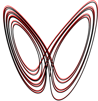
Figure 1: A trajectory of the Lorenz attractor under a shadow coordinate transform. The black trajectory shows $x(t)$, and the red trajectory shows $x^{\prime}(t)$. The perturbation $\epsilon\,\delta x$ shown corresponds to an infinitesimal change in the parameter $r$, and is explained in detail in Section 7.

Now consider a trajectory $x(t)$ satisfying an ordinary differential equation

$$\dot{x}=f(x)\;,$$ (4)

with a smooth vector field $f(x)$ as a function of $x$. The same trajectory in the transformed “shadow” coordinates $x^{\prime}(t)$ do not satisfy the same differential equation. Instead, from Equation (3), we obtain

$$\begin{split}\dot{x^{\prime}}&=f(x)+\epsilon\,\frac{\partial\delta x}{\partial x}\cdot f(x)\\ &=f(x^{\prime})-\epsilon\,\frac{\partial f}{\partial x}\cdot\delta x(x^{\prime})+\epsilon\,\frac{\partial\delta x}{\partial x}\cdot f(x^{\prime})+O(\epsilon^{2})\end{split}$$ (5)

In other words, the shadow trajectory $x^{\prime}(t)$ satisfies a slightly perturbed equation

$$\dot{x^{\prime}}=f(x^{\prime})+\epsilon\,\delta f(x^{\prime})+O(\epsilon^{2})$$ (6)

where the perturbation $\delta f$ is

$$\begin{split}\delta f(x)&=-\frac{\partial f}{\partial x}\cdot\delta x(x)+\frac{\partial\delta x}{\partial x}\cdot f(x)\\ &=-\frac{\partial f}{\partial x}\cdot\delta x(x)+\frac{d\delta x}{dt}\\ :&=(S_{f}\delta x)(x)\end{split}$$ (7)

For a given differential equation $\dot{x}=f(x)$, Equation (7) defines a linear operator $S_{f}:\delta x\Rightarrow\delta f$. We call $S_{f}$ the “Shadow Operator” of $f$. For any smooth vector field $\delta x(x)$ that defines a slightly distorted “shadow” coordinate system in the state space, $S_{f}$ determines a unique smooth vector field $\delta f(x)$ that defines a perturbation to the differential equation. Any trajectory of the original differential equation would satisfy the perturbed equation in the distorted coordinates.

Given an ergodic dynamical system $\dot{x}=f(x)$, and a pair $(\delta x,\delta f)$ that satisfies $\delta f=S_{f}\delta x$, $\delta x$ determines the sensitivity of statistical quantities of the dynamical system to an infinitesimal perturbation $\epsilon\delta f$. Let $J(x)$ be a smooth scalar function of the state, consider the statistical average $\langle J\rangle$ as defined in Equation (1). The sensitivity derivative of $\langle J\rangle$ to the infinitesimal perturbation $\epsilon\,\delta f$ is by definition

$$\frac{d\langle J\rangle}{d\epsilon}=\lim_{\epsilon\rightarrow 0}\frac{1}{\epsilon}\left(\lim_{T\rightarrow\infty}\frac{1}{T}\int_{0}^{T}J(x^{\prime}(t))\,dt-\lim_{T\rightarrow\infty}\frac{1}{T}\int_{0}^{T}J(x(t))\,dt\right)$$ (8)

where by the ergodicity assumption, the statistical average of the perturbed system can be computed by averaging over $x^{\prime}(t)$, which satisfies the perturbed governing differential equation. Continuing from Equation (8),

$$\begin{split}\frac{d\langle J\rangle}{d\epsilon}&=\lim_{\epsilon\rightarrow 0}\lim_{T\rightarrow\infty}\frac{1}{T}\int_{0}^{T}\frac{J(x^{\prime}(t))-J(x(t))}{\epsilon}\>dt\\ &=\lim_{T\rightarrow\infty}\lim_{\epsilon\rightarrow 0}\frac{1}{T}\int_{0}^{T}\frac{J(x^{\prime}(t))-J(x(t))}{\epsilon}\>dt\\ &=\lim_{T\rightarrow\infty}\frac{1}{T}\int_{0}^{T}\frac{\partial J}{\partial x}\cdot\delta x\>dt=\left\langle\frac{\partial J}{\partial x}\cdot\delta x\right\rangle\;.\end{split}$$ (9)

Equation (9) represents the sensitivity derivative of a statistical quantity $\langle J\rangle$ to the size of a perturbation $\epsilon\delta f$. There are two subtle points here:

• The two limits $\lim_{\epsilon\rightarrow 0}$ and $\lim_{T\rightarrow\infty}$ can commute with each other for the following reason: The two trajectories $x^{\prime}(t)$ and $x(t)$ stay uniformly close to each other forever; therefore,

  $$\frac{J(x^{\prime}(t))-J(x(t))}{\epsilon}\overset{\epsilon\rightarrow 0}{\longrightarrow}\frac{\partial J}{\partial x}\cdot\delta x$$ (10)

  uniformly for all $t$. Consequently,

  $$\frac{1}{T}\int_{0}^{T}\frac{J(x^{\prime}(t))-J(x(t))}{\epsilon}\>dt\overset{\epsilon\rightarrow 0}{\longrightarrow}\frac{1}{T}\int_{0}^{T}\frac{\partial J}{\partial x}\cdot\delta x\;dt$$ (11)

  uniformly for all $T$. Thus the two limits commute.

• The two trajectories $x^{\prime}(t)$ and $x(t)$ start at two specially positioned pair of initial conditions $x^{\prime}(0)=x(0)+\epsilon\,\delta x(x(0))$. Almost any other pair of initial conditions (e.g. $x^{\prime}(0)=x(0)$) would make the two trajectories diverge as a result of the “butterfly effect”. They would not stay uniformly close to each other, and the limits $\lim_{\epsilon\rightarrow 0}$ and $\lim_{T\rightarrow\infty}$ would not commute.

Equation (9) represents the sensitivity derivative of the statistical quantity $\langle J\rangle$ to the infinitesimal perturbation $\epsilon\,\delta f$ as another statistical quantity $\langle\frac{\partial J}{\partial x}\cdot\delta x\rangle$. We can compute it by averaging $\frac{\partial J}{\partial x}\cdot\delta x$ over a sufficiently long trajectory, provided that $\delta x=S^{-1}\delta f$ is known along the trajectory. The next section describes how to numerically compute $\delta x=S^{-1}\delta f$ for a given $\delta f$.

3 Inverting the Shadow Operator

Perturbations to input parameters can often be represented as perturbations to the dynamics. Consider a differential equation $\dot{x}=f(x,s_{1},s_{2},\ldots,s_{m})$ parameterized by $m$ input variables, an infinitesimal perturbation in a input parameter $s_{j}\rightarrow s_{j}+\epsilon$ can be represented as a perturbation to the dynamics $\epsilon\,\delta f=\epsilon\,\frac{df}{ds_{j}}$.

Equation (9) defines the sensitivity derivative of the statistical quantity $\langle J\rangle$ to an infinitesimal perturbation $\epsilon\,\delta f$, provided that a $\delta x$ can be found satisfying $\delta f=S_{f}\delta x$, where $S_{f}$ is the shadow operator. To compute the sensitivity by evaluating Equation (9), one must first numerically invert $S_{f}$ for a given $\delta f$ to find the corresponding $\delta x$.

The key ingredient of numerical inversion of $S_{f}$ is the Lyapunov spectrum decomposition. This decomposition can be efficiently computed numerically [11] [2]. In particular, we focus on the case when the system $\dot{x}=f(x)$ has distinct Lyapunov exponents. Denote the Lyapunov covariant vectors as $\phi_{1}(x),\phi_{2}(x),\ldots,\phi_{n}(x)$. Each $\phi_{i}$ is a vector field in the state space satisfying

$$\frac{d}{dt}\phi_{i}(x(t))=\frac{\partial f}{\partial x}\cdot\phi_{i}(x(t))-\lambda_{i}\phi_{i}(x(t))$$ (12)

where $\lambda_{1},\lambda_{2},\ldots,\lambda_{n}$ are the Lyapunov exponents in decreasing order.

The Lyapunov spectrum decomposition enables a divide and conquer strategy for computing $\delta x=S_{f}^{-1}\delta f$. For any $\delta f(x)$ and every point $x$ on the attractor, both $\delta x(x)$ and $\delta f(x)$ can be decomposed into the Lyapunov covariant vector directions almost everywhere, i.e.

$$\delta x(x)=\sum_{i=1}^{n}a^{x}_{i}(x)\,\phi_{i}(x)\;,$$ (13)

$$\delta f(x)=\sum_{i=1}^{n}a^{f}_{i}(x)\,\phi_{i}(x)\;,$$ (14)

where $a^{x}_{i}$ and $a^{f}_{i}$ are scalar fields in the state space. From the form of $S_{f}$ in Equation (7), we obtain

$$\begin{split}S_{f}(a^{x}_{i}\phi_{i})=&-\frac{\partial f}{\partial x}\cdot(a^{x}_{i}(x)\phi_{i}(x))+\frac{d}{dt}(a^{x}_{i}(x)\,\phi_{i}(x))\\ =&-a^{x}_{i}(x)\>\frac{\partial f}{\partial x}\cdot\phi_{i}(x)+\frac{d\,a^{x}_{i}(x)}{dt}\,\phi_{i}(x)+a^{x}_{i}(x)\>\frac{d\,\phi_{i}(x)}{dt}\;.\end{split}$$ (15)

By substituting Equation (12) into the last term of Equation (15), we obtain

$$S_{f}(a^{x}_{i}\phi_{i})=\left(\frac{da^{x}_{i}(x)}{dt}-\lambda_{i}\,a^{x}_{i}(x)\right)\,\phi_{i}(x)\;,$$ (16)

By combining Equation (16) with Equations (13), (14) and the linear relation $\delta f=S_{f}\delta x$, we finally obtain

$$\delta f=\sum_{i=1}^{n}S_{f}(a^{x}_{i}\phi_{i})=\sum_{i=1}^{n}\;\underbrace{\left(\frac{da^{x}_{i}}{dt}-\lambda_{i}\,a^{x}_{i}\right)}_{\displaystyle a^{f}_{i}}\,\phi_{i}\;,$$ (17)

Equations (16) and (17) are useful for two reasons:

1. They indicate that the Shadow Operator $S_{f}$, applied to a scalar field $a^{x}_{i}(x)$ multiple of $\phi_{i}(x)$, generates another scalar field $a^{f}_{i}(x)$ multiple of the same vector field $\phi_{i}(x)$. Therefore, one can compute $S_{f}^{-1}\delta f$ by first decomposing $\delta f$ as in Equation (14) to obtain the $a^{f}_{i}$. If each $a_{i}^{x}$ can be calculated from the corresponding $a_{i}^{f}$, then $\delta x$ can be computed with Equation (13), completing the inversion.

2. It defines a scalar ordinary differential equation that governs the relation between $a^{x}_{i}$ and $a^{f}_{i}$ along a trajectory $x(t)$:

   $$\frac{da^{x}_{i}(x)}{dt}=a^{f}_{i}(x)+\lambda_{i}\,a^{x}_{i}(x)$$ (18)

   This equation can be used to obtain $a^{x}_{i}$ from $a^{f}_{i}$ along a trajectory, thereby filling the gap in the inversion procedure of $S_{f}$ outlined above. For each positive Lyapunov exponent $\lambda_{i}$, one can integrate the ordinary differential equation

   $$\frac{d\check{a}^{x}_{i}}{dt}=\check{a}^{f}_{i}+\lambda_{i}\,\check{a}^{x}_{i}$$ (19)

   backwards in time from an arbitrary terminal condition, and the difference between $\check{a}^{x}_{i}(t)$ and the desired $a^{x}_{i}(x)$ will decrease exponentially. For each negative Lyapunov exponent $\lambda_{i}$, Equation (19) can be integrated forward in time from an arbitrary initial condition, and $\check{a}^{x}_{i}(t)$ will converge exponentially to the desired $a^{x}_{i}(x)$. For a zero Lyapunov exponent $\lambda_{i}=0$, Section 4 introduces a solution.

4 Time Dilation and Compression

There is a fundamental problem in the inversion method derived in Section 3: $S_{f}$ is not invertible for certain $\delta f$. This can be shown with the following analysis: Any continuous time dynamical system with a non-trivial attractor must have a zero Lyapunov exponent $\lambda_{n_{0}}=0$. The corresponding Lyapunov covariant vector is $\phi_{n_{0}}(x)=f(x)$. This can be verified by substituting $\lambda_{i}=0$ and $\phi_{i}=f$ into Equation (12). For this $i=n_{0}$, Equations (19) becomes

$$a^{f}_{n_{0}}(x)=\frac{da^{x}_{n_{0}}(x)}{dt}$$ (20)

By taking an infinitely long time average on both sides of Equation (20), we obtain

$$\left\langle a^{f}_{n_{0}}(x)\right\rangle=\lim_{T\rightarrow\infty}\frac{a^{x}_{n_{0}}(x(T))-a^{x}_{n_{0}}(x(0))}{T}=0\;,$$ (21)

Equation (21) implies that for any $\delta f=S_{f}\delta x$, the $i=n_{0}$ component of its Lyapunov decomposition (as in Equation (14)) must satisfy $\langle a^{f}_{n_{0}}(x)\rangle=0$. Any $\delta f$ that do not satisfy this linear relation, e.g. $\delta f\equiv f$, would not be in the range space of $S_{f}$. Thus the corresponding $\delta x=S_{f}^{-1}\delta f$ does not exist.

Our solution to the problem is complementing $S_{f}$ with a “global time dilation and compression” constant $\eta$, whose effect produces a $\delta f$ that is outside the range space of $S_{f}$. We call $\eta$ a time dilation constant for short. The combined effect of a time dilation constant and a shadow transform could produce all smooth perturbations $\delta f$.

The idea comes from the fact that for a constant $\eta$, the time dilated or compressed system $\dot{x}=(1+\epsilon\,\eta)f(x)$ has exactly the same statistics $\langle J\rangle$, as defined in Equation (1), as the original system $\dot{x}=f(x)$. Therefore, the perturbation in any $\langle J\rangle$ due to any $\epsilon\,\delta f$ is equal to the perturbation in $\langle J\rangle$ due to $\epsilon\,(\eta f(x)+\delta f(x))$. Therefore, the sensitivity derivative to $\delta f$ can be computed if we can find a $\delta x$ that satisfies $S_{f}\delta x=\eta f(x)+\delta f(x)$ for some $\eta$.

We use the “free” constant $\eta$ to put $\eta f(x)+\delta f(x)$ into the range space of $S_{f}$. By substituting $\eta f(x)+\delta f(x)$ into the constraint Equation (21) that identifies the range space of $S_{f}$, the appropriate $\eta$ must satisfy the following equation

$$\eta+\langle a^{f}_{n_{0}}\rangle=0\;,$$ (22)

which we use to numerically compute $\eta$.

Once the appropriate time dilation constant $\eta$ is computed, $\eta f(x)+\delta f(x)$ is in the range space of $S_{f}$. We use the procedure in Section 3 to compute $\delta x=S_{f}^{-1}(\eta f+\delta f)$, then use Equation (9) to compute the desired sensitivity derivative $d\langle J\rangle/d\epsilon$. The addition of $\eta f$ to $\delta f$ affects Equation (19) only for $i=n_{0}$, making it

$$\frac{da^{x}_{n_{0}}(x)}{dt}=a^{f}_{n_{0}}(x)+\eta\;.$$ (23)

Equation (23) indicates that $a^{x}_{n_{0}}$ can be computed by integrating the right hand side along the trajectory.

The solution to Equation (23) admits an arbitrary additive constant. The effect of this arbitrary constant is the following: By substituting Equations (13) into Equation (9), the contribution from the $i=n_{0}$ term of $\delta x$ to $d\langle J\rangle/d\epsilon$ is

$$\lim_{T\rightarrow\infty}\frac{1}{T}\int_{0}^{T}a^{f}_{n_{0}}\frac{dJ}{dt}\,dt$$ (24)

Therefore, any constant addition to $a^{f}_{n_{0}}$ vanishes as $T\rightarrow\infty$. Computationally, however, Equation (9) must be approximated by a finite time average. We find it beneficial to adjust the level of $a^{f}_{n_{0}}$ to approximately $\langle a^{f}_{n_{0}}\rangle=0$, in order to control the error due to finite time averaging.

5 The Forward Sensitivity Analysis Algorithms

For a given $\dot{x}=f(x)$, $\delta f$ and $J(x)$, the mathematical developments in Sections 3 and 4 are summarized into Algorithm 1 for computing the sensitivity derivative $d\delta\langle J\rangle/d\epsilon$ as in Equation (9).

Algorithm 1 The Forward Sensitivity Analysis Algorithm

1. Choose a “spin-up buffer time” $T_{B}$, and an “statistical averaging time” $T_{A}$. $T_{B}$ should be much longer than $1/|\lambda_{i}|$ for all nonzero Lyapunov exponent $\lambda_{i}$, so that the solutions of Equation (19) can reach $a_{i}^{x}$ over a time span of $T_{B}$. $T_{A}$ should be much longer than the decorrelation time of the dynamics, so that one can accurately approximate a statistical quantity by averaging over $[0,T_{A}]$.

2. Obtain an initial condition on the attractor at $t=-T_{B}$, e.g., by solving $\dot{x}=f(x)$ for a sufficiently long time span, starting from an arbitrary initial condition.

3. Solve $\dot{x}=f(x)$ to obtain a trajectory $x(t),t\in[-T_{B},T_{A}+T_{B}]$; compute the Lyapunov exponents $\lambda_{i}$ and the Lyapunov covariant vectors $\phi_{i}(x(t))$ along the trajectory, e.g., using algorithms in [11] and [2].

4. Perform the Lyapunov spectrum decomposition of $\delta f(x)$ along the trajectory $x(t)$ to obtain $a^{f}_{i}(x),i=1,\ldots,n$ as in Equation (14).

5. Compute the global time dilation constant $\eta$ using Equation (22).

6. Solve the differential equations (19) to obtain $a^{x}_{i}$ over the time interval $[0,T_{A}]$. The equations with positive $\lambda_{i}$ are solved backward in time from $t=T_{A}+T_{B}$ to $t=0$; the ones with negative $\lambda_{i}$ are solved forward in time from $t=-T_{B}$ to $t=T_{A}$. For $\lambda_{n_{0}}=0$, Equation (23) is integrated, and the mean of $a^{x}_{n_{0}}$ is set to zero.

7. Compute $\delta x$ along the trajectory $x(t),t\in[0,T_{A}]$ with Equation (13).

8. Compute $d\langle J\rangle/d\epsilon$ using Equation (1) by averaging over the time interval $[0,T_{A}]$.

The preparation phase of the algorithm (Steps 1-3) computes a trajectory and the Lyapunov spectrum decomposition along the trajectory. The algorithm then starts by decomposing $\delta f$ (Step 4), followed by computing $\delta x$ (Steps 5-7), and finally computing $d\langle J\rangle/d\epsilon$ (Step 8). The sensitivity derivative of many different statistical quantities $\langle J_{1}\rangle,\langle J_{2}\rangle,\ldots$ to a single $\delta f$ can be computed by only repeating the last step of the algorithm. Therefore, this is a “forward” algorithm in the sense that it efficiently computes sensitivity of multiple output quantities to a single input parameter (the size of perturbation $\epsilon\,\delta f$). We will see that this is in sharp contrast to the “adjoint” algorithm described in Section 6, which efficiently computes the sensitivity derivative of one output statistical quantity $\langle J\rangle$ to many perturbations $\delta f_{1},\delta f_{2},\ldots$.

It is worth noting that the $\delta x$ computed using Algorithm 1 satisfies the forward tangent equation

$$\dot{\delta x}=\frac{\partial f}{\partial x}\cdot\delta x+\eta\,f+\delta f$$ (25)

This can be verified by taking derivative of Equation (13), substituting Equations (19) and (23), then using Equation (14). However, $\delta x$ must satisfy both an initial condition and a terminal condition, making it difficult to solve with conventional time integration methods. In fact, Algorithm 1 is equivalent to splitting $\delta x$ into stable, neutral and unstable components, corresponding to positive, zero and negative Lyapunov exponents; then solving Equation (25) separately for each component in different time directions. This alternative version of the forward sensitivity computation algorithm could be useful for large systems to avoid computation of all the Lyapunov covariant vectors.

6 The Adjoint Sensitivity Analysis Algorithm

The adjoint algorithm starts by trying to find an adjoint vector field $\hat{f}(x)$, such that the sensitivity derivative of the given statistical quantity $\langle J\rangle$ to any infinitesimal perturbation $\epsilon\,\delta f$ can be represented as

$$\frac{d\langle J\rangle}{\epsilon}=\left\langle\hat{f\,}^{T}\cdot\delta f\right\rangle$$ (26)

Both $\hat{f}$ in Equation (26) and $\frac{\partial J}{\partial x}$ in Equation (9) can be decomposed into linear combinations of the adjoint Lyapunov covariant vectors almost everywhere on the attractor:

$$\hat{f}(x)=\sum_{i=1}^{n}{\hat{a}}^{f}_{i}(x)\,\psi_{i}(x)\;,$$ (27)

$$\frac{\partial J}{\partial x}^{T}=\sum_{i=1}^{n}{\hat{a}}^{x}_{i}(x)\,\psi_{i}(x)\;,$$ (28)

where the adjoint Lyapunov covariant vectors $\psi_{i}$ satisfy

$$-\frac{d}{dt}\psi_{i}(x(t))=\frac{\partial f}{\partial x}^{T}\cdot\psi_{i}(x(t))-\lambda_{i}\psi_{i}(x(t))$$ (29)

With proper normalization, the (primal) Lyapunov covariant vectors $\phi_{i}$ and the adjoint Lyapunov covariant vectors $\psi_{i}$ have the following conjugate relation:

$$\psi_{i}(x)^{T}\cdot\phi_{j}(x)\equiv\begin{cases}0\;,&i\neq j\\ 1\;,&i=j\end{cases}$$ (30)

i.e., the $n\times n$ matrix formed by all the $\phi_{i}$ and the $n\times n$ matrix formed by all the $\psi_{i}$ are the transposed inverse of each other at every point $x$ in the state space.

By substituting Equations (13) and (28) into Equation (9), and using the conjugate relation in Equation (30), we obtain

$$\frac{d\langle J\rangle}{d\epsilon}=\sum_{i=1}^{n}\left\langle{\hat{a}}_{i}^{x}a_{i}^{x}\right\rangle$$ (31)

Similarly, by combining Equations (26), (14), (27) and (30), it can be shown that $\hat{f}$ satisfies Equation (26) if and only if

$$\frac{d\langle J\rangle}{d\epsilon}=\sum_{i=1}^{n}\left\langle{\hat{a}}_{i}^{f}a_{i}^{f}\right\rangle$$ (32)

Comparing Equations (31) and (32) leads to the following conclusion: Equation (26) can be satisfied by finding ${\hat{a}}_{i}^{f}$ that satisfy

$$\left\langle{\hat{a}}_{i}^{f}a_{i}^{f}\right\rangle=\left\langle{\hat{a}}_{i}^{x}a_{i}^{x}\right\rangle\;,\quad i=1,\ldots,n$$ (33)

The ${\hat{a}}_{i}^{f}$ that satisfies Equation (33) can be found using the relation between $a_{i}^{f}$ and $a_{i}^{x}$ in Equation (18). By multiplying $\hat{a}_{i}^{f}$ on both sides of Equation (18) and integrate by parts in time, we obtain

$$\frac{1}{T}\int_{0}^{T}{\hat{a}}_{i}^{f}a_{i}^{f}dt=\left.\frac{{\hat{a}}_{i}^{f}a_{i}^{x}}{T}\right|_{0}^{T}-\frac{1}{T}\int_{0}^{T}\left(\frac{d{\hat{a}}_{i}^{f}}{dt}+\lambda_{i}\,{\hat{a}}_{i}^{f}\right)a^{x}_{i}\;dt$$ (34)

for $i\neq n_{0}$. Through apply the same technique to Equation (23), we obtain for $i=n_{0}$

$$\frac{1}{T}\int_{0}^{T}{\hat{a}}_{n_{0}}^{f}a_{n_{0}}^{f}dt=\left.\frac{{\hat{a}}_{n_{0}}^{f}a_{n_{0}}^{x}}{T}\right|_{0}^{T}-\frac{1}{T}\int_{0}^{T}\frac{d{\hat{a}}_{n_{0}}^{f}}{dt}\,a^{x}_{n_{0}}dt+\frac{1}{T}\int_{0}^{T}\eta\,\hat{a}^{f}_{n_{0}}dt$$ (35)

If we set $\hat{a}_{i}^{f}$ to satisfy the following relations

$$-\frac{d{\hat{a}}_{i}^{f}(x)}{dt} =\hat{a}_{i}^{x}(x)+\lambda_{i}\,{\hat{a}}_{i}^{f}(x)\;, i\neq n_{0}\;,$$ (36)

$$-\frac{d{\hat{a}}_{i}^{f}(x)}{dt} =\hat{a}_{i}^{x}(x)\;,\quad\langle\hat{a}_{i}^{f}\rangle=0\;,\quad i=n_{0}\;,$$

then Equations (34) and (35) become

$$\frac{1}{T}\int_{0}^{T}{\hat{a}}_{i}^{f}a_{i}^{f}dt =\left.\frac{{\hat{a}}_{i}^{f}a_{i}^{x}}{T}\right|_{0}^{T}+\frac{1}{T}\int_{0}^{T}\hat{a}_{i}^{x}a_{i}^{x}\;dt\;,\quad i\neq n_{0}$$ (37)

$$\frac{1}{T}\int_{0}^{T}{\hat{a}}_{i}^{f}a_{i}^{f}dt =\left.\frac{{\hat{a}}_{i}^{f}a_{i}^{x}}{T}\right|_{0}^{T}+\frac{1}{T}\int_{0}^{T}\hat{a}_{i}^{x}a_{i}^{x}\;dt+\eta\left(\frac{1}{T}\int_{0}^{T}\hat{a}^{f}_{n_{0}}\,dt-\langle\hat{a}^{f}_{n_{0}}\rangle\right), i=n_{0}$$

As $T\rightarrow\infty$, both equations reduces to Equation (33).

In summary, if the scalar fields $\hat{a}_{i}^{f}$ satisfy Equation (36), then they also satisfy Equation (37) and thus Equation (33); as a result, the $\hat{f}$ formed by these $\hat{a}^{f}$ through Equation (27) satisfies Equation (26), thus is the desired adjoint vector field.

For each $i\neq n_{0}$, the scalar field $\hat{a}_{i}^{f}$ satisfying Equation (36) can be computed by solving an ordinary differential equations

$$-\frac{d\check{\hat{a}}_{i}^{f}}{dt}=\check{\hat{a}}_{i}^{x}+\lambda_{i}\,\check{\hat{a}}_{i}^{f}\;.$$ (38)

Contrary to computation of $a_{i}^{x}$ through solving Equation (19), the time integration should be forward in time for positive $\lambda_{i}$, and backward in time for negative $\lambda_{i}$, in order for the difference between $\check{\hat{a}}_{i}^{f}(t)$ and ${\hat{a}}_{i}^{f}(x(t))$ to diminish exponentially.

The $i=n_{0}$ equation in Equation (36) can be directly integrated to obtain ${\hat{a}}_{n_{0}}^{f}(x)$. The equation is well defined because the right hand side is mean zero:

$$\frac{1}{T}\int_{0}^{T}\hat{a}_{n_{0}}^{f}(x(t))\,dt=\frac{1}{T}\int_{0}^{T}\frac{\partial J}{\partial x}\cdot\phi_{n_{0}}\,dt=\frac{1}{T}\int_{0}^{T}\frac{dJ}{dt}\,dt\overset{T\rightarrow\infty}{\longrightarrow}0\;.$$ (39)

Therefore, the integral of ${\hat{a}}_{n_{0}}^{x}(x)$ over time, subtracted by its mean, is the solution ${\hat{a}}_{n_{0}}^{f}(x)$ to the $i=n_{0}$ case of Equation (36).

Algorithm 2 The Adjoint Sensitivity Analysis Algorithm

1. Choose a “spin-up buffer time” $T_{B}$, and an “statistical averaging time” $T_{A}$. $T_{B}$ should be much longer than $1/|\lambda_{i}|$ for all nonzero Lyapunov exponent $\lambda_{i}$, so that the solutions of Equation (19) can reach $a_{i}^{x}$ over a time span of $T_{B}$. $T_{A}$ should be much longer than the decorrelation time of the dynamics, so that one can accurately approximate a statistical quantity by averaging over $[0,T_{A}]$.

2. Obtain an initial condition on the attractor at $t=-T_{B}$, e.g., by solving $\dot{x}=f(x)$ for a sufficiently long time span, starting from an arbitrary initial condition.

3. Solve $\dot{x}=f(x)$ to obtain a trajectory $x(t),t\in[-T_{B},T_{A}+T_{B}]$; compute the Lyapunov exponents $\lambda_{i}$ and the Lyapunov covariant vectors $\phi_{i}(x(t))$ along the trajectory, e.g., using algorithms in [11] and [2].

4. Perform the Lyapunov spectrum decomposition of $(\partial J/\partial x)^{T}$ along the trajectory $x(t)$ to obtain $\hat{a}^{x}_{i}(x(t)),i=1,\ldots,n$ as in Equation (28).

5. Solve the differential equations (38) to obtain $\hat{a}_{i}^{f}(x(t))$ over the time interval $[0,T_{A}]$. The equations with negative $\lambda_{i}$ are solved backward in time from $t=T_{A}+T_{B}$ to $t=0$; the ones with positive $\lambda_{i}$ are solved forward in time from $t=-T_{B}$ to $t=T_{A}$. For $i=n_{0}$, the scalar $-a^{x}_{n_{0}}$ is integrated along the trajectory; the mean of the integral is subtracted from the integral itself to obtain $\hat{a}^{f}_{n_{0}}$.

6. Compute $\hat{f}$ along the trajectory $x(t),t\in[0,T_{A}]$ with Equation (27).

7. Compute $d\langle J\rangle/d\epsilon$ using Equation (26) by averaging over the time interval $[0,T_{A}]$.

The above analysis summarizes to Algorithm 2 for computing the sensitivity derivative derivative of the statistical average $\langle J\rangle$ to an infinitesimal perturbations $\epsilon\,\delta f$. The preparation phase of the algorithm (Steps 1-3) is exactly the same as in Algorithm 1. These steps compute a trajectory $x(t)$ and the Lyapunov spectrum decomposition along the trajectory. The adjoint algorithm then starts by decomposing the derivative vector $(\partial J/\partial x)^{T}$ (Step 4), followed by computing the adjoint vector $\delta f$ (Steps 5-6), and finally computing $d\langle J\rangle/d\epsilon$ for a particular $\delta f$. Note that the sensitivity of the same $\langle J\rangle$ to many different perturbations $\delta f_{1},\delta f_{2},\ldots$ can be computed by repeating only the last step of the algorithm. Therefore, this is an “adjoint” algorithm, in the sense that it efficiently computes the sensitivity derivatives of a single output quantity to many input perturbation.

It is worth noting that $\hat{f}$ computed using Algorithm 2 satisfies the adjoint equation

$$-\dot{\hat{f}}=\frac{\partial f}{\partial x}^{T}\cdot\hat{f}-\frac{\partial J}{\partial x}$$ (40)

This can be verified by taking derivative of Equation (27), substituting Equation (36), then using Equation (28). However, $\hat{f}$ must satisfy both an initial condition and a terminal condition, making it difficult to solve with conventional time integration methods. In fact, Algorithm 2 is equivalent to splitting $\hat{f}$ into stable, neutral and unstable components, corresponding to positive, zero and negative Lyapunov exponents; then solving Equation (40) separately for each component in different time directions. This alternative version of the adjoint sensitivity computation algorithm could be useful for large systems, to avoid computation of all the Lyapunov covariant vectors.

7 An Example: the Lorenz Attractor

We consider the Lorenz attractor $\dot{x}=f(x)$, where $x=(x_{1},x_{2},x_{3})^{T}$, and

$$f(x)=\left(\begin{array}[]{c}\sigma(x_{2}-x_{1})\\ x_{1}(r-x_{3})-x_{2}\\ x_{1}x_{2}-\beta x_{3}\end{array}\right)$$ (41)

The “classic” parameter values $\sigma=10$, $r=28$, $\beta=8/3$ are used. Both the forward sensitivity analysis algorithm (Algorithm 1) and the adjoint sensitivity analysis algorithm (Algorithm 2) are performed on this system.

We want to demonstrate the computational efficiency of our algorithm; therefore, we choose a relatively short statistical averaging interval of $T_{A}=10$, and a spin up buffer period of $T_{B}=5$. Only a single trajectory of length $T_{A}+2T_{B}$ on the attractor is required in our algorithm. Considering that the oscillation period of the Lorenz attractor is around $1$, the combined trajectory length of $20$ is a reasonable time integration length for most simulations of chaotic dynamical systems. In our example, we start the time integration from $t=-10$ at $x=(-8.67139571762,4.98065219709,25)$, and integrate the equation to $t=-5$, to ensure that the entire trajectory from $-T_{B}$ to $T_{A}+T_{B}$ is roughly on the attractor. The rest of the discussion in this section are focused on the trajectory $x(t)$ for $t\in[-T_{B},T_{A}+T_{B}]$.

7.1 Lyapunov covariant vectors

The Lyapunov covariant vectors are computed in Step 3 of both Algorithm 1 and Algorithm 2, over the time interval $[-T_{B},T_{A}+T_{B}]$. These vectors, along with the trajectory $x(t)$, are shown in Figure 2.

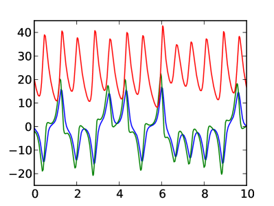
(a) The state vector $x$

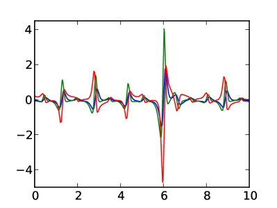
(b) First Lyapunov covariant vector $\phi_{1}$

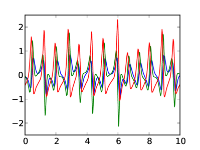
(c) Second Lyapunov covariant vector $\phi_{2}$

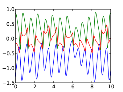
(d) Third Lyapunov covariant vector $\phi_{3}$

Figure 2: The Lyapunov covariant vectors of the Lorenz attractor along the trajectory $x(t)$ for $t\in[0,10]$. The x-axes are $t$; the blue, green and red lines correspond to the $x_{1},x_{2}$ and $x_{3}$ coordinates in the state space, respectively.

The three dimensional Lorenz attractor has three pairs of Lyapunov exponents and Lyapunov covariant vectors. $\lambda_{1}$ is the only positive Lyapunov exponent, and $\phi_{1}$ is computed by integrating the tangent linear equation

$$\dot{\tilde{x}}=\frac{\partial f}{\partial x}\cdot\tilde{x}$$ (42)

forward in time from an arbitrary initial condition at $t=-T_{B}$. The first Lyapunov exponent is estimated to be $\lambda_{1}\approx 0.95$ through a linear regression of $\tilde{x}$ in the log space. The first Lyapunov vector is then obtained as $\phi_{1}=\tilde{x}\,e^{-\lambda_{1}t}$.

$\lambda_{2}=0$ is the vanishing Lyapunov exponent; therefore, $\phi_{2}=\theta\,f(x)$, where $\theta=1/\sqrt{\langle\|f\|_{2}^{2}\rangle}$ is a normalizing constant that make the mean magnitude of $\phi_{2}$ equal to 1.

The third Lyapunov exponent $\lambda_{3}$ is negative. So $\phi_{3}$ is computed by integrating the tangent linear equation (42) backwards in time from an arbitrary initial condition at $t=T_{A}+T_{B}$. The third Lyapunov exponent is estimated to be $\lambda_{3}\approx-14.6$ through a linear regression of the backward solution $\tilde{x}$ in the log space. The third Lyapunov vector is then obtained as $\phi_{3}=\tilde{x}\,e^{-\lambda_{3}t}$.

7.2 Forward Sensitivity Analysis

We demonstrate our forward sensitivity analysis algorithm by computing the sensitivity derivative of three statistical quantities $\langle x_{1}^{2}\rangle$, $\langle x_{2}^{2}\rangle$ and, $\langle x_{3}\rangle$ to a small perturbation in the system parameter $r$ in the Lorenz attractor Equation (41). The infinitesimal perturbation $r\rightarrow r+\epsilon$ is equivalent to the perturbation

$$\epsilon\,\delta f=\epsilon\,\frac{\partial f}{\partial r}=\epsilon\,(0,x_{1},0)^{T}\;.$$ (43)

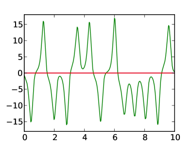
(a) $\delta f=\dfrac{df}{dr}$

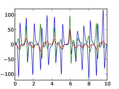
(b) $a^{f}_{i},i=1,2,3$ for the $\delta f$

Figure 3: Lyapunov vector decomposition of $\delta f$. The x-axes are $t$; the blue, green and red lines on the left are the first, second and third component of $\delta f$ as defined in Equation (43); the blue, green and red lines on the right are $a^{f}_{1}$, $a^{f}_{2}$ and $a^{f}_{3}$ in the decomposition of $\delta f$ (Equation (14)), respectively.

The forcing term defined in Equation (43) is plotted in Figure 3a. Figure 3b plots the decomposition coefficients $a_{i}^{f}$, computed by solving a $3\times 3$ linear system defined in Equation (14) at every point on the trajectory.

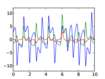
(a) $a^{x}_{i},i=1,2,3$ for the $\delta f$

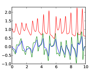
(b) $\delta x=\sum_{i=1}^{3}a^{x}_{i}\,\phi_{i}$

Figure 4: Inversion of $S_{f}$ for $\delta x=S_{f}^{-1}\delta f$. The x-axes are $t$; the blue, green and red lines on the left are $a^{x}_{1}$, $a^{x}_{2}$ and $a^{x}_{3}$, respectively; the blue, green and red lines on the right are the first, second and third component of $\delta x$, computed via Equation (13).

For each $a^{f}_{i}$ obtained through the decomposition, Equation (19) or (23) is solved to obtain $a^{x}_{i}$. For $i=1$, Equation (19) is solved backwards in time from $t=T_{A}+T_{B}$ to $t=0$. For $i=n_{0}=2$, the time compression constant is estimated to be $\eta\approx-2.78$, and Equation (23) is integrated to obtain $a^{x}_{2}$. For $i=3$, Equation (19) is solved forward in time from $t=-T_{B}$ to $t=T_{A}$.

The resulting values of $a^{x}_{i},i=1,2,3$ are plotted in Figure 4a. These values are then substituted into Equation (13) to obtain $\delta x$, as plotted in Figure 4b. The “shadow” trajectory defined as $x^{\prime}=x+\epsilon\delta x$ is also plotted in Figure 1 as the red lines, for an $\epsilon=1/3$. This $\delta x=S_{f}^{-1}\delta f$ is approximately the shadow coordinate perturbation “induced” by a $1/3$ increase in the input parameter $r$, a.k.a. the Rayleigh number in the Lorenz attractor.

The last step of the forward sensitivity analysis algorithm is computing the sensitivity derivatives of the output statistical quantities using Equation (9). We found that using a windowed time averaging [4] yields more accurate sensitivities. Here our estimates over the time interval $[0,T_{A}]$ are

$$\frac{d\langle x_{1}^{2}\rangle}{dr}\approx 2.64\;,\quad\frac{d\langle x_{2}^{2}\rangle}{dr}\approx 3.99\;,\quad\frac{d\langle x_{3}\rangle}{dr}\approx 1.01$$ (44)

These sensitivity values compare well to results obtained through finite difference, as shown in Section 7.4.

7.3 Adjoint Sensitivity Analysis

We demonstrate our adjoint sensitivity analysis algorithm by computing the sensitivity derivatives of the statistical quantity $\langle x_{3}\rangle$ to small perturbations in the three system parameters $s$, $r$ and $b$ in the Lorenz attractor Equation (41).

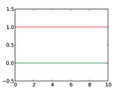
(a) $\dfrac{\partial J}{\partial x}$ for $J=x_{3}$

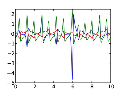
(b) $\hat{a}^{x}_{i},i=1,2,3$ for the $\dfrac{\partial J}{\partial x}$

Figure 5: Adjoint Lyapunov vector decomposition of $\partial J/\partial x$. The x-axes are $t$; the blue, green and red lines on the left are the first, second and third component of $\partial J/\partial x$; the blue, green and red lines on the right are $\hat{a}^{x}_{1}$, $\hat{a}^{x}_{2}$ and $\hat{a}^{x}_{3}$ in the decomposition of $\partial J/\partial x$ (Equation (28)), respectively.

The first three steps of Algorithm 2 is the same as in Algorithm 1, and has been demonstrated in Section 7.1. Step 4 involves decomposing $(\partial J/\partial x)^{T}$ into three adjoint Lyapunov covariant vectors. In our case, $J(x)=x_{3}$, therefore $\partial J/\partial x\equiv(0,0,1)$, as plotted in Figure 5a. The adjoint Lyapunov covariant vectors $\psi_{i}$ can be computed using Equation (30) by inverting the $3\times 3$ matrix formed by the (primal) Lyapunov covariant vectors $\phi_{i}$ at every point on the trajectory. The coefficients $\hat{a}^{x}_{i},i=1,2,3$ can then be computed by solving Equation (28). These scalar quantities along the trajectory are plotted in Figure 5b for $t\in[0,T_{A}]$.

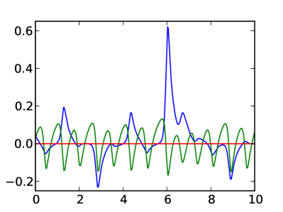
(a) $\hat{a}^{f}_{i},i=1,2,3$ solved using Equation (38)

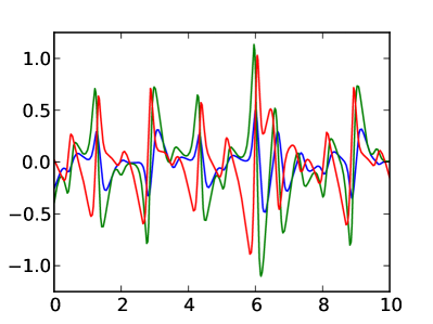
(b) $\hat{f}=\sum_{i=1}^{3}\hat{a}^{f}_{i}\,\psi_{i}$

Figure 6: Computation of the adjoint solution $\hat{f}$ for the Lorenz attractor. The x-axes are $t$; the blue, green and red lines on the left are $\hat{a}^{f}_{1}$, $\hat{a}^{f}_{2}$ and $\hat{a}^{f}_{3}$, respectively; the blue, green and red lines on the right are the first, second and third component of $\hat{f}$, computed via Equation (27).

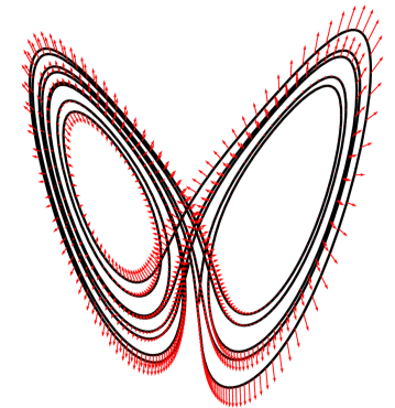
Figure 7: The adjoint sensitivity derivative $\hat{f}$ as in Equation (26), represented by arrows on the trajectory.

Once we obtain $\hat{a}_{i}^{x}$, $\hat{a}_{i}^{f}$ can be computed by solving Equation (38). The solution is plotted in Figure 6a. Equation (27) can then be used to combine the $\hat{a}_{i}^{f}$ into the adjoint vector $\hat{f}$. The computed $\hat{f}$ along the trajectory is plotted both in Figure 6b as a function of $t$, and also in Figure 7 as arrows on the trajectory in the state space.

The last step of the adjoint sensitivity analysis algorithm is computing the sensitivity derivatives of $\langle J\rangle$ to the perturbations $\delta f_{s}=\frac{df}{ds}$, $\delta f_{r}=\frac{df}{dr}$ and $\delta f_{b}=\frac{df}{db}$ using Equation (26). Here our estimates over the time interval $[0,T_{A}]$ are computed as

$$\frac{d\langle x_{3}\rangle}{ds}\approx 0.21\;,\quad\frac{d\langle x_{3}\rangle}{dr}\approx 0.97\;,\quad\frac{d\langle x_{3}\rangle}{db}\approx-1.74$$ (45)

Note that $\frac{d\langle x_{3}\rangle}{dr}$ estimated using adjoint method differs from the same value estimated using forward method (44). This discrepancy can be caused by the different numerical treatments to the time dilation term in the two methods. The forward method numerically estimates the time dilation constant $\eta$ through Equation (22); while the adjoint method sets the mean of $\hat{a}_{i}^{f}$ to zero (36), so that the computation is independent to the value of $\eta$. This difference could cause apparent discrepancy in the estimated sensitivity derivatives.

The next section compares these sensitivity estimates, together with the sensitivity estimates computed in Section 7.2, to a finite difference study.

7.4 Comparison with the finite difference method

To reduce the noise in the computed statistical quantities in the finite difference study, a very long time integration length of $T=100,000$ is used for each simulation. Despite this long time averaging, the quantities computed contain statistical noise of the order $0.01$. The noise limits the step size of the finite difference sensitivity study. Fortunately all the output statistical quantities seem fairly linear with respect to the input parameters, and a moderately large step size of the order $0.1$ can be used. To further reduce the effect of statistical noise, we perform linear regressions through $10$ simulations of the Lorenz attractor, with $r$ equally spaced between $27.9$ and $28.1$. The total time integration length (excluding spin up time) is $1,000,000$. The resulting computation cost is in sharp contrast to our method, which involves a trajectory of only length $20$.

Similar analysis is performed for the parameters $s$ and $b$, where 10 values of $s$ equally spaced between $9.8$ and $10.2$ are used, and 10 values of $b$ equally spaced between $8/3-0.02$ and $8/3+0.02$ are used. The slopes estimated from the linear regressions, together with $3\sigma$ confidence intervals (where $\sigma$ is the standard error of the linear regression) is listed below:

$$\begin{split}&\frac{d\langle x_{1}^{2}\rangle}{dr}=2.70\pm 0.10\;,\quad\frac{d\langle x_{2}^{2}\rangle}{dr}=3.87\pm 0.18\;,\quad\frac{d\langle x_{3}\rangle}{dr}=1.01\pm 0.04\\ &\frac{d\langle x_{3}\rangle}{ds}=0.16\pm 0.02\;,\quad\frac{d\langle x_{3}\rangle}{db}=-1.68\pm 0.15\;.\end{split}$$ (46)

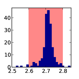
(a) $\dfrac{\partial\langle x_{1}^{2}\rangle}{\partial r}$

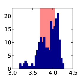
(b) $\dfrac{\partial\langle x_{2}^{2}\rangle}{\partial r}$

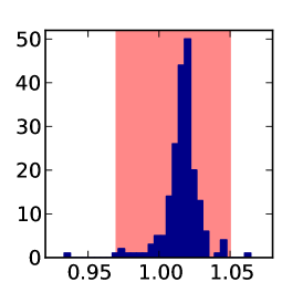
(c) $\dfrac{\partial\langle x_{3}\rangle}{\partial r}$

Figure 8: Histogram of sensitivities computed using Algorithm 1 (forward sensitivity analysis) starting from 200 random initial conditions. $T_{A}=10,T_{B}=5$. The red region identifies the $3\sigma$ confidence interval estimated using finite difference regression.

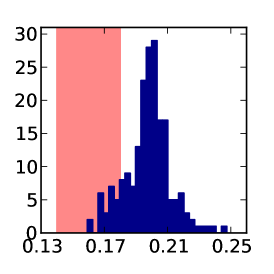
(a) $\dfrac{\partial\langle x_{3}\rangle}{\partial s}$

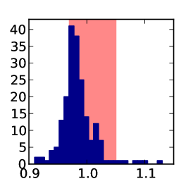
(b) $\dfrac{\partial\langle x_{3}\rangle}{\partial r}$

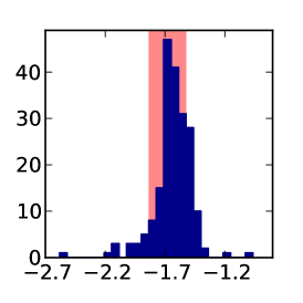
(c) $\dfrac{\partial\langle x_{3}\rangle}{\partial b}$

Figure 9: Histogram of sensitivities computed using Algorithm 2 (adjoint sensitivity analysis) starting from 200 random initial conditions. $T_{A}=10,T_{B}=5$. The red region identifies the $3\sigma$ confidence interval estimated using finite difference regression.

To further assess the accuracy of our algorithm, which involves finite time approximations to Equations (9) and (26), we repeated both Algorithm 1 and Algorithm 2 for 200 times, starting from random initial conditions at $T=-10$. We keep the statistical averaging time $T_{A}=10$ and the spin up buffer time $T_{B}=5$. The resulting histogram of sensitivities computed with Algorithm 1 is shown in Figure 8; the histogram of sensitivities computed with Algorithm 2 is shown in Figure 9. The finite difference estimates are also indicated in these plots.

We observe that our algorithms compute accurate sensitivities most of the time. However, some of the computed sensitivities seems to have heavy tails in their distribution. This may be due to behavior of the Lorenz attractor near the unstable fixed point $(0,0,0)$. Similar heavy tailed distribution has been observed in other studies of the Lorenz attractor [1]. They found that certain quantities computed on Lorenz attractor can have unbounded second moment. This could be the case in our sensitivity estimates. Despite this minor drawback, the sensitivities computed using our algorithm have good quality. Our algorithms are much more efficient than existing sensitivity computation methods using ensemble averages.

8 Conclusion

This paper derived a forward algorithm and an adjoint algorithm for computing sensitivity derivatives in chaotic dynamical systems. Both algorithms efficiently compute the derivative of statistical quantities $\langle J\rangle$ to infinitesimal perturbations $\epsilon\,\delta f$ to the dynamics.

The forward algorithm starts from a given perturbation $\delta f$, and computes a perturbed “shadow” coordinate system $\delta x$, e.g. as shown in Figure 1. The sensitivity derivatives of multiple statistical quantities to the given $\delta f$ can be computed from $\delta x$. The adjoint algorithm starts from a statistical quantity $\langle J\rangle$, and computes an adjoint vector $\hat{f}$, e.g. as shown in Figure 7. The sensitivity derivative of the given $\langle J\rangle$ to multiple input perturbations can be computed from $\hat{f}$.

We demonstrated both the forward and adjoint algorithms on the Lorenz attractor at standard parameter values. The forward sensitivity analysis algorithm is used to simultaneously compute $\frac{\partial\langle x_{1}^{2}\rangle}{\partial r}$, $\frac{\partial\langle x_{2}^{2}\rangle}{\partial r}$, and $\frac{\partial\langle x_{3}\rangle}{\partial r}$; the adjoint sensitivity analysis algorithm is used to simultaneously compute $\frac{\partial\langle x_{3}\rangle}{\partial s}$, $\frac{\partial\langle x_{3}\rangle}{\partial r}$, and $\frac{\partial\langle x_{3}\rangle}{\partial b}$. We show that using a single trajectory of length about $20$, both algorithms can efficiently compute accurate estimates of all the sensitivity derivatives.

References

- [1] G. Eyink, T. Haine, and D. Lea. Ruelle’s linear response formula, ensemble adjoint schemes and Lévy flights. Nonlinearity, 17:1867–1889, 2004.
- [2] F. Ginelli, P. Poggi, A. Turchi, H. Chaté, R. Livi, and A. Politi. Characterizing dynamics with covariant Lyapunov vectors. Physical Review Letters, 99:130601, Sep 2007.
- [3] A. Jameson. Aerodynamic design via control theory. Journal of Scientific Computing, 3:233–260, 1988.
- [4] J. Krakos, Q. Wang, S. Hall, and D. Darmofal. Sensitivity analysis of limit cycle oscillations. Journal of Computational Physics, (0):–, 2012.
- [5] D. Lea, M. Allen, and T. Haine. Sensitivity analysis of the climate of a chaotic system. Tellus, 52A:523–532, 2000.
- [6] D. Ruelle. Differentiation of SRB states. Communications in Mathematical Physics, 187:227–241, 1997.
- [7] D. Ruelle. A review of linear response theory for general differentiable dynamical systems. Nonlinearity, 22(4):855, 2009.
- [8] J.-N. Thepaut and P. Courtier. Four-dimensional variational data assimilation using the adjoint of a multilevel primitive-equation model. Quarterly Journal of the Royal Meteorological Society, 117(502):1225–1254, 1991.
- [9] D. Venditti and D. Darmofal. Grid adaptation for functional outputs: Application to two-dimensional inviscid flow. Journal of Computational Physics, 176:40–69, 2002.
- [10] Q. Wang, P. Moin, and G. Iaccarino. Minimal repetition dynamic checkpointing algorithm for unsteady adjoint calculation. SIAM Journal on Scientific Computing, 31(4):2549–2567, 2009.
- [11] C. Wolfe and R. Samelson. An efficient method for recovering Lyapunov vectors from singular vectors. Tellus A, 59(3):355–366, 2007.