${\mathbf{T}}$-odd Momentum Correlation in Radiative ${\mathbf{\beta}}$ Decay

Abstract

We consider neutron radiative $\beta$ decay, $n\rightarrow pe^{-}\bar{\nu}_{e}\gamma$, and compute the T-odd momentum correlation in the decay rate characterized by the kinematical variable $\xi={\mathbf{l}}_{\nu}\cdot({\mathbf{l}}_{e}\times{\mathbf{k}})$ arising from electromagnetic final-state interactions in the Standard Model. Our expression for the corresponding T-odd asymmetry $A_{\xi}^{\rm SM}$ is exact in ${\cal O}(\alpha)$ up to terms of recoil order, and we evaluate it numerically under various kinematic conditions. Noting the universality of the V-A law in the absence of recoil-order terms, we retain the parametric dependence on masses and coupling constants throughout, so that our results serve as a template for the computation of $A_{\xi}^{\rm SM}$ in allowed nuclear radiative $\beta$ decays and hyperon radiative $\beta$ decays as well.

I Introduction

Radiative $\beta$ decay offers the opportunity of studying T-odd momentum correlations which do not appear in ordinary $\beta$ decay Jackson:1957zz . We consider a correlation characterized by the kinematical variable $\xi={\mathbf{l}}_{\nu}\cdot({\mathbf{l}}_{e}\times{\mathbf{k}})$, so that it is both parity P and naively time-reversal T odd but independent of the particle spin. Its spin independence renders it distinct from searches for permanent electric-dipole moments (EDMs) of neutrons and nuclei. The inability of the Standard Model (SM) to explain the cosmic baryon asymmetry prompts the search for sources of CP violation which do not appear within it and which are not constrained by other experiments. A triple momentum correlation in radiative $\beta$ decay is one such example, as we shall illustrate; under the CPT theorem, T violation is linked to CP violation. A decay correlation, however, can be, by its very nature, only “naively” or “pseudo” T odd, that is, only motion-reversal odd. As a result, although the appearance of a T-odd decay correlation can be engendered by sources of CP violation beyond the Standard Model, it can also be generated without fundamental T or CP violation. In this paper we compute the size of the T-odd momentum correlation in radiative $\beta$ decay simulated by electromagnetic final-state interactions in the SM sachs . This is crucial to establishing a baseline in the search for new sources of CP violation in such processes. Our work is motivated in large part by the determination that pseudo-Chern-Simons terms appear in SU(2)${}_{\rm L}\times$U(1) gauge theories at low energies – and that they can impact low-energy weak radiative processes involving baryons Harvey:2007rd ; Harvey:2007ca ; Hill:2009ek . In the SM such pseudo-Chern-Simons interactions are CP conserving, but considered broadly they are not, so that searching for the P- and T-odd effects that CP-violating interactions of pseudo-Chern-Simons form would engender offers a new window on physics beyond the SM svgdh1 .

Searches for T-violating decay correlations in neutron and nuclear $\beta$ decay have a long history. The best experimental limits are on the so-called $D$ term, which appears as the triple correlation $D{\mathbf{S}}\cdot({\mathbf{l}}_{e}\times{\mathbf{l}}_{\nu})$, where ${\mathbf{S}}$ is the polarization of the decaying particle Mumm:2011nd ; calaprice . These limits still greatly exceed the size of the $D$ correlation expected from SM final-state interactions Callan:1967zz ; Ando:2009jk . Radiative $\beta$ decay offers the possibility of forming a T-odd correlation from momenta alone; to our knowledge such a possibility was first considered in the context of $K_{l3\gamma}^{+}$ decay braguta . The T-odd asymmetry computed in Ref. braguta from electromagnetic final-state interactions has recently been recalculated and is in significant disagreement with the earlier result khriprud .

In this paper we evaluate the T-odd asymmetry in radiative $\beta$ decay from electromagnetic radiative corrections in the SM and focus on the neutron case: $n(p_{n})\rightarrow p(p_{p})+e^{-}(l_{e})+\bar{\nu}_{e}(l_{\nu})+\gamma(k)$. The motion-reversal-odd terms in the decay rate, which mimic the appearance of T violation, are engendered by the interference of the tree-level amplitude with the imaginary part of the ${\cal O}(\alpha)$ corrected amplitude, which is determined by the physical two-particle cuts and hence mediated by the scattering of particles on their mass shells Cutkosky:1960sp ; Callan:1967zz ; Okun:1967ww . In what follows, we detail the computation of the interference terms and their components, as well as the resulting numerical integration over the allowed phase space to yield the T-odd asymmetry $A_{\xi}^{\rm SM}$. Our results are exact in ${\cal O}(\alpha)$ up to corrections of recoil order, namely, up to terms of ${\cal O}(\varepsilon/M)$, where $\varepsilon$ is an energy scale which is small with respect to the nucleon mass $M$. This certitude is guaranteed by the small $Q$ value of the decay, so that $\varepsilon\ll M$, and by Low’s theorem Low:1958sn . The natural scale of hadron excitations is set by the pion mass $m_{\pi}$; consequently, in neutron radiative $\beta$ decay $\varepsilon\ll m_{\pi}$ as well, and nonelectromagnetic final-state interactions cannot contribute to the physical two-particle cuts. This is in contradistinction to $K_{l3\gamma}^{+}$ decay for which such contributions are appreciable, albeit relatively small Muller:2006gu . We relegate intermediate results essential for our final results but yet nonessential to the flow of our discussion to Appendixes. Since we neglect all terms of recoil order, our results are relevant to the computation of $A_{\xi}^{\rm SM}$ in nuclear and hyperon radiative $\beta$ decays as well. We assess the size of undetermined corrections before offering a final summary of our results.

II Formalism

We work in a simultaneous expansion in the electromagnetic coupling constant $e$ and in $\varepsilon/M$, so that the leading contributions to neutron radiative $\beta$ decay are from the diagrams in Fig. 1. At this order the baryons are effectively structureless, and the contributions arise from bremsstrahlung off the charged particle legs of ordinary $\beta$ decay, yielding a gauge-invariant result Low:1958sn .

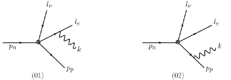
Figure 1: Contributions to $n(p_{n})\to p(p_{p})+e^{-}(l_{e})+{\bar{\nu}}_{e}(l_{\nu})+\gamma(k)$ up to corrections of recoil order. The effective weak vertex is denoted by $\otimes$ and is controlled by the Fermi constant $G_{\rm F}$. The diagram enumeration is utilized in our calculation of the T-odd asymmetry.

Employing the notation and conventions of Ref. PS , the decay amplitude is:

$${\cal M}_{\rm tree}={\cal M}_{01}+{\cal M}_{02}\,,$$ (1)

with gaponov ; bgmz

$${\cal M}_{01}(l_{e},k,p_{p}) = \frac{eg_{V}G_{F}}{\sqrt{2}}\bar{u}_{e}(l_{e})\frac{2l_{e}\cdot\epsilon^{\ast}+\not{\epsilon}^{\ast}\not{k}}{2l_{e}\cdot k}\gamma_{\rho}(1-\gamma_{5})v_{\nu}(l_{\nu})\bar{u}_{p}(p_{p})\gamma^{\rho}(1-\lambda\gamma_{5})u_{n}(p_{n})\,,$$ (2)

$${\cal M}_{02}(l_{e},k,p_{p}) = -\frac{eg_{V}G_{F}}{\sqrt{2}}\bar{u}_{e}(l_{e})\gamma_{\rho}(1-\gamma_{5})v_{\nu}(l_{\nu})\bar{u}_{p}(p_{p})\frac{2p_{p}\cdot\epsilon^{\ast}+\not{\epsilon}^{\ast}\not{k}}{2p_{p}\cdot k}\gamma^{\rho}(1-\lambda\gamma_{5})u_{n}(p_{n})\,,$$ (3)

where $\epsilon^{\mu}$ is the photon polarization vector and $\lambda\equiv g_{A}/g_{V}$, noting that $g_{V}$ and $g_{A}$ are the vector and axial-vector weak coupling constants of the nucleon, respectively. We explicitly include the arguments in the momenta $l_{e}$, $k$, and $p_{p}$ for later convenience.

The branching ratio and photon energy spectrum for this process have been computed previously gaponov ; bgmz . The expressions which follow from Eq. (2) are consistent with the experimental results nico ; cooper . The next-to-leading order terms in the small-scale expansion, i.e., those of ${\cal O}(\varepsilon/M)$, have been computed in heavy-baryon chiral perturbation theory and are no larger than ${\cal O}(0.5\%)$ of the leading-order result bgmz – this is some 20 times smaller than the current experimental sensitivity cooper . In what follows we neglect all recoil-order terms and consider the ${\cal O}(\alpha)$ corrections to the amplitude of Eq. (2). For future reference, employing lepton and hadron tensors, we note that bgmz

$$\sum_{\rm spins}|{\cal M}_{0}|^{2}=\frac{e^{2}g^{2}_{V}G^{2}_{F}}{2}\left(\frac{1}{(l_{e}\cdot k)^{2}}L^{\rm ee}_{\rho\delta}H^{\rho\delta}+\frac{1}{M_{p}^{2}\omega^{2}}L^{\rho\delta}H^{\rm ee}_{\rho\delta}-\frac{1}{M_{p}\omega(l_{e}\cdot k)}M^{\rm ee,mixed}\right)\,,$$ (4)

where $M_{n}$, $M_{p}$, and $\omega$ refer to the neutron mass, the proton mass, and the photon energy, respectively, and

$$L^{\rm ee}_{\rho\delta}H^{\rho\delta} = -64M_{n}M_{p}\left(m^{2}_{e}-l_{e}\cdot k\right)\left((1+3\lambda^{2})E_{\nu}(E_{e}+\omega)+(1-\lambda^{2})({\bf l}_{e}\cdot{\bf l}_{\nu}+{\bf l}_{\nu}\cdot{\bf k})\right)\,,$$

$$L^{\rho\delta}H^{\rm ee}_{\rho\delta} = -64M_{n}M_{p}^{3}\left((1+3\lambda^{2})E_{\nu}E_{e}+(1-\lambda^{2}){\bf l}_{e}\cdot{\bf l}_{\nu}\right)\,,$$ (5)

$$M^{\rm ee,mixed} = -64M_{n}M_{p}^{2}\left((1+3\lambda^{2})E_{\nu}(2E_{e}^{2}+E_{e}\omega-l_{e}\cdot k)+(1-\lambda^{2})E_{e}(2{\bf l}_{e}\cdot{\bf l}_{\nu}+{\bf l}_{\nu}\cdot{\bf k})\right)\,,$$

with $m_{e}$ the electron mass. In realizing the amplitudes from the Feynman rules we impose $\epsilon_{i}(k)\cdot k=0$ for each polarization state $i$ of a real photon with momentum $k$, noting $\sum_{i=1,2}\epsilon_{i}^{\ast}(k)\cdot\epsilon_{i}(k)=-2$. To effect the subsequent photon polarization sums, however, we employ QED gauge invariance and make the replacement $\sum_{i=1,2}\epsilon_{i}^{\mu}(k)\epsilon_{i}^{\nu\,\ast}(k)\longrightarrow-g^{\mu\nu}$ throughout, without any supplemental conditions.

Denoting the ${\cal O}(\alpha)$ correction to the amplitude by ${\cal M}_{\rm loop}$ the amended decay rate is determined by

$$|{\cal M}|^{2}=|{\cal M}_{\rm tree}|^{2}+{\cal M}_{\rm tree}\cdot{{\cal M}^{\ast}_{\rm loop}}+{{\cal M}_{\rm loop}}\cdot{{\cal M}^{\ast}_{\rm tree}}+{\cal O}(\alpha^{2})\,.$$ (6)

The T-odd triple momenta correlation $\xi={\mathbf{l}}_{\nu}\cdot({\mathbf{l}}_{e}\times{\mathbf{k}})$ in the decay rate can arise from the interference between the tree-level amplitude ${\cal M}_{\rm tree}$ and the anti-Hermitian parts of the one-loop corrections to it, so that ultimately the interference term $\sum_{\rm spins}(2{\rm Re}({\cal M}_{\rm tree}{\cal M}^{\ast}_{\rm loop}))$ contains terms linear in $\xi$. Since we consider the decay and detection of unpolarized particles exclusively, $\sum_{\rm spins}|{\cal M}|^{2}_{\rm{\bf T}\ odd}$ is indeed characterized by terms linear in $\xi$. Evidently the induced asymmetry is suppressed by a factor of $\alpha\equiv e^{2}/4\pi\sim 1/137$; explicit computation shows it to be much smaller still.

Before turning to the computation of $|{\cal M}|^{2}_{\rm{\bf T}\ odd}$ let us consider its relation to a measurable quantity. Following Ref. braguta , we define a T-odd asymmetry $A_{\xi}$, namely,

$$A_{\xi}=\frac{N_{+}-N_{-}}{N_{+}+N_{-}}\,,$$ (7)

where $N_{+}$ is defined as the total number of decay events with positive $\xi$, and $N_{-}$ is defined as the number of events with negative $\xi$. Specifically, we compute

$$A_{\xi}=\frac{\Gamma_{+}-\Gamma_{-}}{\Gamma_{+}+\Gamma_{-}}\,,$$ (8)

where $\Gamma_{\pm}$ contains an integral of $|{\cal M}|^{2}$ over the region of phase space with $\xi\stackrel{{\scriptstyle>}}{{{}_{<}}}0$, respectively; the numerator is nonzero if and only if $|{\cal M}|^{2}_{\rm{\bf T}\ odd}$ is nonzero. Working to corrections of ${\cal O}(\varepsilon/M)$, the neutron radiative $\beta$-decay rate $\Gamma$ in the neutron rest frame is

$$\Gamma=\frac{1}{8M_{n}}\frac{1}{(2\pi)^{8}}\int|{\mathbf{l}}_{e}|d{E_{e}}d{\Omega_{e}}\omega d{\omega}d{\Omega_{k}}d{\Omega_{\nu}}\frac{\Theta(M_{n}-E_{e}-E_{\nu}-\omega)E_{\nu}}{4M_{n}}\left(\frac{1}{2}\sum_{\rm spins}|{\cal M}|^{2}\right)\Bigg{|}_{p_{p},\,E_{\nu}}\,,$$ (9)

where $p_{p}=M_{n}-l_{e}-l_{\nu}-k$ and $E_{\nu}=M_{n}-M_{p}-E_{e}-\omega$ are fixed throughout. The precise form of $\Gamma_{\pm}$ depends on the concrete choice of coordinate system. Choosing the direction of the electron momentum ${\mathbf{l}}_{e}$ as the ${\mathbf{z}}$ direction and letting ${\mathbf{k}}$ and ${\mathbf{l}}_{e}$ fix the $\mathbf{x}$-$\mathbf{z}$ plane, then under this specific choice $\xi>0$ corresponds to $\phi_{\nu}\in[0,\pi]$ and $\xi<0$ corresponds to $\phi_{\nu}\in[\pi,2\pi]$. Thus we define

$$\Gamma_{+}(\omega^{\rm min})\equiv\frac{1}{16M_{n}^{2}(2\pi)^{6}}\int^{\omega^{\rm max}}_{\omega^{\rm min}}\omega d\omega\int^{E_{e}^{\rm max}(\omega)}_{m_{e}}|{\mathbf{l}}_{e}|dE_{e}\int^{\rm c}_{\rm-c}dx_{k}\int^{1}_{-1}dx_{\nu}\int^{\pi}_{0}d\phi_{\nu}E_{\nu}$$

$$\times\left(\frac{1}{2}\sum_{\rm spins}|{\cal M}|^{2}\right)\Bigg{|}_{p_{p},\,E_{\nu}}\,,$$ (10)

and

$$\Gamma_{-}(\omega^{\rm min})\equiv\frac{1}{16M_{n}^{2}(2\pi)^{6}}\int^{\omega^{\rm max}}_{\omega^{\rm min}}\omega d\omega\int^{E_{e}^{\rm max}(\omega)}_{m_{e}}|{\mathbf{l}}_{e}|dE_{e}\int^{\rm c}_{\rm-c}dx_{k}\int^{1}_{-1}dx_{\nu}\int^{2\pi}_{\pi}d\phi_{\nu}E_{\nu}$$

$$\times\left(\frac{1}{2}\sum_{\rm spins}|{\cal M}|^{2}\right)\Bigg{|}_{p_{p},\,E_{\nu}}\,,$$ (11)

where $E_{e}^{\rm max}=M_{n}-M_{p}-\omega$, $\omega^{\rm max}=M_{n}-M_{p}-m_{e}$, and $\omega^{\min}$ is determined by the threshold energy of the detector. In our computation of $|{\cal M}|^{2}$ we set $M_{n}=M_{p}=M$ in terms which would yield corrections beyond leading order in the recoil expansion. We limit the integration over $x_{k}$ to the range $[-{\rm c},{\rm c}]$; we discuss this as well as our choice for ${\rm c}$ in Sec. IV.

III Computation of $\sum_{\rm spins}\mathbf{|{\cal M}|^{2}_{{\bf T}\ odd}}$ in leading order

To compute the T-odd pieces, we need to obtain the anti-Hermitian parts of the one-loop diagrams ${\rm Im}({\cal M}_{\rm loop})$. We do this by performing “Cutkosky cuts” Cutkosky:1960sp , which means we simultaneously put intermediate particles in the loops on their mass shells in all physically allowed ways and then perform the relevant intermediate phase-space integrals and spin sums. Graphically speaking, after imposing the cuts, the anti-Hermitian part of a one-loop diagram can be viewed as the product of two physical tree-level processes. We have

$${\rm Im}({\cal M}_{\rm loop})=\frac{1}{8\pi^{2}}\sum_{n}\int d\rho_{n}\sum_{s_{n}}{\cal M}_{fn}{{\cal M}^{\ast}_{in}}=\frac{1}{8\pi^{2}}\sum_{n}\int d\rho_{n}\sum_{s_{n}}{\cal M}_{fn}{{\cal M}_{ni}}\,,$$ (12)

where $\sum_{n}$ refers to the summation over all the possible cuts of the one-loop diagrams and $\int d\rho_{n}$ and $\sum_{s_{n}}$ refer to the intermediate phase space integration and spin sums, respectively, for a cut which yields state $n$. The matrix elements ${\cal M}_{ni}$ and ${\cal M}_{fn}$ refer to the two tree-level diagrams after a physical cut. After excluding the physically unacceptable cuts, 14 cut diagrams remain, and they are illustrated in Fig. 2. We evaluate them explicitly. The momenta labeled as $k^{\prime},\,l_{e}^{\prime}$, and $p_{p}^{\prime}$ refer to momenta of intermediate particles. In performing the Cutkosky cuts, each particle in a pair of particles is put on its own mass shell.

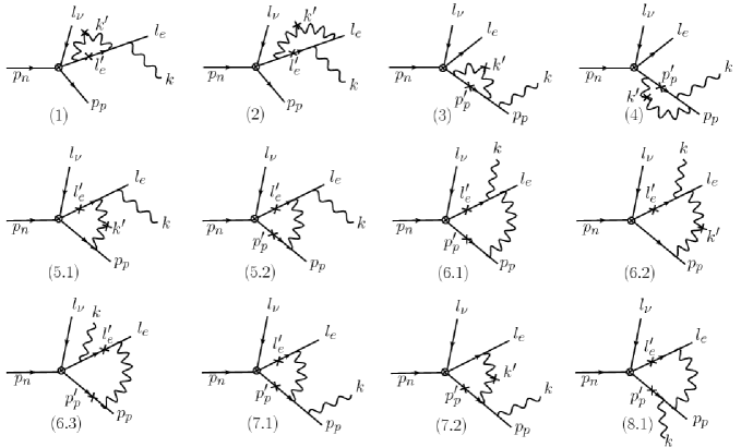
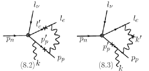
Figure 2: All two-particle cut contributions to $n(p_{n})\to p(p_{p})+e^{-}(l_{e})+{\bar{\nu}}_{e}(l_{\nu})+\gamma(k)$ which appear in ${\cal O}(\alpha)$ up to corrections of recoil order, using the syntax of Fig. 1. A “$\times$” means that the intermediate particle has been put on its mass shell; two such symbols define the Cutkosky cut. The diagram enumeration is utilized in our calculation of the T-odd asymmetry. Note that the first number selects a particular Feynman diagram, and the second determines the particular two-particle physical cut in that diagram.

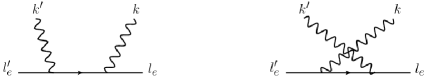
Figure 3: Compton scattering diagrams which appear in ${\rm Im}({\cal M}_{\rm loop})$ for $\gamma-e$ cuts. We denote the two graphs by ${\cal M}^{\rm d}_{\gamma e}(l^{\prime}_{e},k^{\prime},l_{e},k)$ and ${\cal M}^{\rm c}_{\gamma e}(l^{\prime}_{e},k^{\prime},l_{e},k)$, respectively. The diagrams and amplitudes appropriate to $\gamma-p$ scattering follow from replacing electron with proton variables.

It is useful to categorize the cuts as per the sorts of processes involved. That is, ${\cal M}_{fn}$ describes the manner in which select particles rescatter, so that we can have Compton scattering or electron-proton scattering, the latter with or without the emission of an additional photon. The family of diagrams given by (1), (2), (5.1), and (6.2) contains Compton scattering from the electron, as illustrated in Fig. 3, whereas the family comprised of (3), (4), (7.2), and (8.3) contains Compton scattering from the proton. In these families ${\cal M}_{fn}$ is captured by one of the following expressions:

$${\cal M}^{\rm d}_{\gamma e}(l^{\prime}_{e},k^{\prime},l_{e},k)=-e^{2}\bar{u}_{e}(l_{e})\frac{2l_{e}\cdot\epsilon^{\ast}+\not{\epsilon}^{\ast}\not{k}}{2l_{e}\cdot k}\not{\epsilon}^{\prime}u_{e}(l^{\prime}_{e})\,,$$ (13)

$${\cal M}^{\rm c}_{\gamma e}(l^{\prime}_{e},k^{\prime},l_{e},k)=e^{2}\bar{u}_{e}(l_{e})\frac{2l_{e}\cdot\epsilon^{\prime}-\not{\epsilon}^{\prime}\not{k^{\prime}}}{2l^{\prime}_{e}\cdot k}\not{\epsilon}^{\ast}u_{e}(l^{\prime}_{e})\,,$$ (14)

$${\cal M}^{\rm d}_{\gamma p}(p^{\prime}_{p},k^{\prime},p_{p},k)=-e^{2}\bar{u}_{p}(p_{p})\frac{2p_{p}\cdot\epsilon^{\ast}+\not{\epsilon}^{\ast}\not{k}}{2p_{p}\cdot k}\not{\epsilon}^{\prime}u_{p}(p^{\prime}_{p})\,,$$ (15)

or

$${\cal M}^{\rm c}_{\gamma p}(p^{\prime}_{p},k^{\prime},p_{p},k)=e^{2}\bar{u}_{p}(p_{p})\frac{2p_{p}\cdot\epsilon^{\prime}-\not{\epsilon}^{\prime}\not{k^{\prime}}}{2p^{\prime}_{p}\cdot k}\not{\epsilon}^{\ast}u_{p}(p^{\prime}_{p})\,,$$ (16)

where $\epsilon^{\prime}\equiv\epsilon(k^{\prime})$. Correspondingly, ${\cal M}_{ni}$ is given by the tree-level neutron radiative $\beta$-decay amplitude, as per the form of ${\cal M}_{01}$ and ${\cal M}_{02}$, with only some of the arguments changed. Technically we define a “family” to be those contributions to the T-odd correlation which cancel among themselves to yield zero when we replace $\epsilon$ or $\epsilon^{\ast}$ by $k$ or $\epsilon^{\prime}$ or $\epsilon^{\prime\ast}$ by $k^{\prime}$ as per the Ward-Takahashi identities.

Furthermore, there is an intermediate phase-space integral over the kinematically allowed phase space. For $\gamma-e$ scattering we have

$$\int d\rho_{\gamma e}\equiv\int\frac{d^{3}{\bf l^{\prime}}_{e}}{2E^{\prime}_{e}}\frac{d^{3}{\bf k^{\prime}}}{2\omega^{\prime}}\delta^{(4)}(l^{\prime}_{e}+k^{\prime}-P_{0e})\,,$$ (17)

with $P_{0e}\equiv l_{e}+k$, whereas for $\gamma-p$ scattering we have

$$\int d\rho_{\gamma p}\equiv\int\frac{d^{3}{\bf p^{\prime}}_{p}}{2E^{\prime}_{p}}\frac{d^{3}{\bf k^{\prime}}}{2\omega^{\prime}}\delta^{(4)}(p^{\prime}_{p}+k^{\prime}-P_{0p})\,,$$ (18)

with $P_{0p}\equiv p_{p}+k$. Collecting the pieces, we have

$${\rm Im}({\cal M}_{1})=\frac{1}{8\pi^{2}}\int d\rho_{\gamma e}\sum_{s_{\gamma e}}{{\cal M}^{d}_{\gamma e}(l^{\prime}_{e},k^{\prime},l_{e},k){\cal M}_{01}(l^{\prime}_{e},k^{\prime},p_{p})}\,,$$ (19)

$${\rm Im}({\cal M}_{2})=\frac{1}{8\pi^{2}}\int d\rho_{\gamma e}\sum_{s_{\gamma e}}{{\cal M}^{c}_{\gamma e}(l^{\prime}_{e},k^{\prime},l_{e},k){\cal M}_{01}(l^{\prime}_{e},k^{\prime},p_{p})}\,,$$ (20)

$${\rm Im}({\cal M}_{5.1})=\frac{1}{8\pi^{2}}\int d\rho_{\gamma e}\sum_{s_{\gamma e}}{{\cal M}^{d}_{\gamma e}(l^{\prime}_{e},k^{\prime},l_{e},k){\cal M}_{02}(l^{\prime}_{e},k^{\prime},p_{p})}\,,$$ (21)

$${\rm Im}({\cal M}_{6.2})=\frac{1}{8\pi^{2}}\int d\rho_{\gamma e}\sum_{s_{\gamma e}}{{\cal M}^{c}_{\gamma e}(l^{\prime}_{e},k^{\prime},l_{e},k){\cal M}_{02}(l^{\prime}_{e},k^{\prime},p_{p})}\,,$$ (22)

for the “$\gamma-e$” cuts, and

$${\rm Im}({\cal M}_{3})=\frac{1}{8\pi^{2}}\int d\rho_{\gamma p}\sum_{s_{\gamma p}}{{\cal M}^{d}_{\gamma p}(p^{\prime}_{p},k^{\prime},p_{p},k){\cal M}_{02}(l_{e},k^{\prime},p^{\prime}_{p})}\,,$$ (23)

$${\rm Im}({\cal M}_{4})=\frac{1}{8\pi^{2}}\int d\rho_{\gamma p}\sum_{s_{\gamma p}}{{\cal M}^{c}_{\gamma p}(p^{\prime}_{p},k^{\prime},p_{p},k){\cal M}_{02}(l_{e},k^{\prime},p^{\prime}_{p})}\,,$$ (24)

$${\rm Im}({\cal M}_{7.2})=\frac{1}{8\pi^{2}}\int d\rho_{\gamma p}\sum_{s_{\gamma p}}{{\cal M}^{d}_{\gamma p}(p^{\prime}_{p},k^{\prime},p_{p},k){\cal M}_{01}(l_{e},k^{\prime},p^{\prime}_{p})}\,,$$ (25)

$${\rm Im}({\cal M}_{8.3})=\frac{1}{8\pi^{2}}\int d\rho_{\gamma p}\sum_{s_{\gamma p}}{{\cal M}^{c}_{\gamma p}(p^{\prime}_{p},k^{\prime},p_{p},k){\cal M}_{01}(l_{e},k^{\prime},p^{\prime}_{p})}\,,$$ (26)

for the $\gamma-p$ cuts.

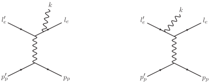
Figure 4: Diagrams which appear in ${\rm Im}({\cal M}_{\rm loop})$ for $e-p$ scattering with electron bremsstrahlung. We denote the two graphs by ${\cal M}^{\rm ef}_{ep\gamma}(l^{\prime}_{e},p^{\prime}_{p},l_{e},k,p_{p})$ and ${\cal M}^{\rm ei}_{ep\gamma}(l^{\prime}_{e},p^{\prime}_{p},l_{e},k,p_{p})$, respectively. The diagrams and amplitudes appropriate to proton bremsstrahlung follow from exchanging electron and proton variables.

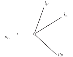
Figure 5: Contribution to $n(p_{n})\to p(p_{p})+e^{-}(l_{e})+{\bar{\nu}}_{e}(l_{\nu})$ decay after Fig. 1.

In addition to the families of Compton cuts, there are cuts in which ${\cal M}_{fn}$ is determined by electron-proton scattering either with and without bremsstrahlung, and, correspondingly, ${\cal M}_{ni}$ is determined by either nonradiative or radiative $\beta$ decay. Referring to Fig. 2, we see for cuts in which the electron and proton scatter with bremsstrahlung that diagrams (5.2) and (6.1) comprise the family associated with electron bremsstrahlung, as shown in Fig. 4, and (7.1) and (8.1) comprise the family associated with proton bremsstrahlung. In these families ${\cal M}_{fn}$ is given by one of the following:

$${\cal M}^{\rm ef}_{ep\gamma}(l^{\prime}_{e},p^{\prime}_{p},l_{e},k,p_{p})=-e^{3}\bar{u}_{e}(l_{e})\frac{2l_{e}\cdot\epsilon^{\ast}+\not{\epsilon}^{\ast}\not{k}}{2l_{e}\cdot k}\gamma^{\mu}u_{e}(l^{\prime}_{e})\frac{g_{\mu\nu}}{(p^{\prime}_{p}-p_{p})^{2}}\bar{u}_{p}(p_{p})\gamma^{\nu}u_{p}(p^{\prime}_{p})\,,$$ (27)

$${\cal M}^{\rm ei}_{ep\gamma}(l^{\prime}_{e},p^{\prime}_{p},l_{e},k,p_{p})=e^{3}\bar{u}_{e}(l_{e})\gamma^{\mu}\frac{2l^{\prime}_{e}\cdot\epsilon^{\ast}-\not{k}\not{\epsilon}^{\ast}}{2l^{\prime}_{e}\cdot k}u_{e}(l^{\prime}_{e})\frac{g_{\mu\nu}}{(p^{\prime}_{p}-p_{p})^{2}}\bar{u}_{p}(p_{p})\gamma^{\nu}u_{p}(p^{\prime}_{p})\,,$$ (28)

$${\cal M}^{\rm pf}_{ep\gamma}(l^{\prime}_{e},p^{\prime}_{p},l_{e},k,p_{p})=e^{3}\bar{u}_{p}(p_{p})\frac{2p_{p}\cdot\epsilon^{\ast}+\not{\epsilon}^{\ast}\not{k}}{2p_{p}\cdot k}\gamma^{\mu}u_{p}(p^{\prime}_{p})\frac{g_{\mu\nu}}{(l^{\prime}_{e}-l_{e})^{2}}\bar{u}_{e}(l_{e})\gamma^{\nu}u_{e}(l^{\prime}_{e})\,,$$ (29)

or

$${\cal M}^{\rm pi}_{ep\gamma}(l^{\prime}_{e},p^{\prime}_{p},l_{e},k,p_{p})=-e^{3}\bar{u}_{p}(p_{p})\gamma^{\mu}\frac{2p^{\prime}_{p}\cdot\epsilon^{\ast}-\not{k}\not{\epsilon}^{\ast}}{2p^{\prime}_{p}\cdot k}u_{p}(p^{\prime}_{p})\frac{g_{\mu\nu}}{(l^{\prime}_{e}-l_{e})^{2}}\bar{u}_{e}(l_{e})\gamma^{\nu}u_{e}(l^{\prime}_{e})\,.$$ (30)

Moreover, ${\cal M}_{ni}$ is given by neutron $\beta$ decay, as shown in Fig. 5, which, up to recoil-order corrections, reads:

$${\cal M}_{\rm DK}(l^{\prime}_{e},p^{\prime}_{p})=\frac{g_{V}G_{F}}{\sqrt{2}}\bar{u}_{e}(l^{\prime}_{e})\gamma_{\rho}(1-\gamma_{5})v_{\nu}(l_{\nu})\bar{u}_{p}(p^{\prime}_{p})\gamma^{\rho}(1-\lambda\gamma_{5})u_{n}(p_{n})\,.$$ (31)

Collecting the pieces, we have

$${\rm Im}({\cal M}_{5.2})=\frac{1}{8\pi^{2}}\int d\rho_{ep\gamma}\sum_{s_{ep}}{{\cal M}^{\rm ef}_{ep\gamma}(l^{\prime}_{e},p^{\prime}_{p},l_{e},k,p_{p}){\cal M}_{\rm DK}(l^{\prime}_{e},p^{\prime}_{p})}\,,$$ (32)

$${\rm Im}({\cal M}_{6.1})=\frac{1}{8\pi^{2}}\int d\rho_{ep\gamma}\sum_{s_{ep}}{{\cal M}^{\rm ei}_{ep\gamma}(l^{\prime}_{e},p^{\prime}_{p},l_{e},k,p_{p}){\cal M}_{\rm DK}(l^{\prime}_{e},p^{\prime}_{p})}\,,$$ (33)

and

$${\rm Im}({\cal M}_{7.1})=\frac{1}{8\pi^{2}}\int d\rho_{ep\gamma}\sum_{s_{ep}}{{\cal M}^{\rm pf}_{ep\gamma}(l^{\prime}_{e},p^{\prime}_{p},l_{e},k,p_{p}){\cal M}_{\rm DK}(l^{\prime}_{e},p^{\prime}_{p})}\,,$$ (34)

$${\rm Im}({\cal M}_{8.1})=\frac{1}{8\pi^{2}}\int d\rho_{ep\gamma}\sum_{s_{ep}}{{\cal M}^{\rm pi}_{ep\gamma}(l^{\prime}_{e},p^{\prime}_{p},l_{e},k,p_{p}){\cal M}_{\rm DK}(l^{\prime}_{e},p^{\prime}_{p})}\,$$ (35)

for the “$e-p-\gamma$” cuts. The last family of cuts is given by (6.3) and (8.2) in Fig. 2. In this case ${\cal M}_{fn}$ is given by $e-p$ scattering, and we have

$${\cal M}_{ep}(l^{\prime}_{e},p^{\prime}_{p},l_{e},p_{p})=-e^{2}\bar{u}_{e}(l_{e})\gamma^{\mu}u_{e}(l^{\prime}_{e})\frac{g_{\mu\nu}}{(l^{\prime}_{e}-l_{e})^{2}}\bar{u}_{p}(p_{p})\gamma^{\nu}u_{p}(p^{\prime}_{p})\,.$$ (36)

The corresponding ${\cal M}_{ni}$ is given by ${\cal M}_{01}(l^{\prime}_{e},k,p^{\prime}_{p})$ for (6.3) and ${\cal M}_{02}(l^{\prime}_{e},k,p^{\prime}_{p})$ for (8.2). We thus have

$${\rm Im}({\cal M}_{6.3})=\frac{1}{8\pi^{2}}\int d\rho_{ep}\sum_{s_{ep}}{{\cal M}_{ep}(l^{\prime}_{e},p^{\prime}_{p},l_{e},p_{p}){\cal M}_{01}(l^{\prime}_{e},k,p^{\prime}_{p})}\,,$$ (37)

$${\rm Im}({\cal M}_{8.2})=\frac{1}{8\pi^{2}}\int d\rho_{ep}\sum_{s_{ep}}{{\cal M}_{ep}(l^{\prime}_{e},p^{\prime}_{p},l_{e},p_{p}){\cal M}_{02}(l^{\prime}_{e},k,p^{\prime}_{p})}\,$$ (38)

for the $e-p$ cuts. In these graphs the intermediate momenta satisfy $l^{\prime}_{e}+p^{\prime}_{p}=l_{e}+p_{p}$, so that the integral over the allowed phase space is slightly different from that in families with $e-p$ scattering and bremsstrahlung. In particular, diagrams (6.3) and (8.2) are each infrared divergent when $l_{e}^{\prime}=l_{e}$; this divergence cancels, however, as expected KLN , once we construct $A_{\xi}^{\rm SM}$.

The expressions we have collected complete the building blocks of the computation of the T-odd correlation in ${\cal O}(\alpha)$ up to recoil-order corrections. The spin-averaged T-odd correlation is

$${\overline{|{\cal M}|^{2}}_{\rm{\bf T}\ odd}}\equiv\frac{1}{2}\sum_{\rm spins}|{\cal M}|^{2}_{\rm{\bf T}\ odd}=\frac{1}{2}\sum_{\rm spins}(2{\rm Re}({\cal M}_{\rm tree}i{\rm Im}{\cal M}^{\ast}_{\rm loop}))\,,$$ (39)

and we report the contributions to it family by family as each family represents a QED gauge-invariant group of contributions. We employ a subscript system to identify the contributions in a straightforward way. Since the T-odd correlations are given by the interference of tree-level diagrams, which are numbered in Fig. 1 as (01) and (02), with one-loop level diagrams, which are numbered in Fig. 2 as (1), (2),…, and (8.3), we label, for example, the T-odd correlation from the tree diagram (01) and one-loop diagram (6.3) as ${\overline{|{\cal M}|^{2}}_{\rm{\bf T}\ odd}}[6.3.01]$. In computing the intermediate phase-space integrals which enter these expresssions, we find that both vector and tensor structures appear in the intermediate momenta. We simplify such integrals using the Passarino-Veltman reduction passvelt and present the details, as well as all needed integrals, in Appendix A. In Appendix B we report concrete expressions for the final gauge-invariant combinations of the various contributions to ${\overline{|{\cal M}|^{2}}_{\rm{\bf T}\ odd}}$ which result after performing the trace calculations and employing the formulas of Appendix A for the intermediate phase-space integrals. We work to leading order in the recoil expansion throughout. Judging by the structure of the resulting expressions one can see that some families, namely, the $\gamma-p$ family containing cuts (3)+(4)+(7.2)+(8.3), as well as the $e-p-\gamma$ family containing cuts (7.1)+(8.1), do not have leading-recoil-order contributions, whereas others do and need to be considered carefully. The computations necessary to determine ${\rm Im}({\cal M}_{\rm loop})$ and the resulting T-odd interference term are involved, so that we employ the program FORM to compute analytic expressions for the traces vermaseren . We compute all of the diagrams with these methods as a check of our procedures – we verify that the expected cancellations do indeed occur.

IV Results

Before presenting our final results for the asymmetry, there are three important remarks to be made concerning our numerical evaluation of the integral of ${\overline{|{\cal M}|^{2}}_{\rm{\bf T}\ odd}}$ over the allowed phase space. First of all, we note that the contributions to the asymmetry from the $e-p$ and $e-p-\gamma$ cuts dominate the final numerical result. The $\gamma-p$ contribution vanishes in leading order, whereas the $\gamma-e$ contribution partially cancels – the latter observation comes from our detailed numerical evaluation of the asymmetry. Second, we note that the contributions from the diagrams of the $e-p$ cuts each contain an infrared divergence; we regulate this by inserting a fictitious photon mass $m_{\gamma}$. However, as we show in Appendix B, the infrared divergence cancels in the net contribution to the asymmetry from the $e-p$ cuts. The remaining piece is thus finite and well-defined, and we can safely set $m_{\gamma}$ to zero. Finally, we note it is most convenient to choose a restricted range in the $\gamma-e$ opening angle. As one can see from the formulas in the Appendix A, the solutions to the Passarino-Veltman equations become invalid if the opening angle $\theta_{e\gamma}$ between the outgoing electron and the photon is exactly equal to 0 or to $\pi$. There is no physical divergence. Rather, the spatial components of the vector and tensor equations to determine the relevant coefficients become degenerate at such a boundary. Potentially one could remove this difficulty by solving the equations for infinitesimal values of $\theta_{e\gamma}$ or $(\theta_{e\gamma}-\pi)$ and then interpolating the solutions to the needed $\theta_{e\gamma}=0$ and $\pi$ points. In our present work, we simply choose a restricted range $x_{k}\equiv\cos\theta_{e\gamma}\in[-0.9,0.9]$, which spans the angular range over which the neutron radiative decay rate is largest byrne .

Table 1: T-odd asymmetry as a function of $\omega_{\rm min}$ for neutron radiative $\beta$ decay.

$\omega_{\rm min}({\rm MeV})$		${A_{\xi}}$
0.01		$1.76\times 10^{-5}$
0.05		$3.86\times 10^{-5}$
0.1		$6.07\times 10^{-5}$
0.2		$9.94\times 10^{-5}$
0.3		$1.31\times 10^{-4}$
0.4		$1.54\times 10^{-4}$
0.5		$1.70\times 10^{-4}$
0.6		$1.81\times 10^{-4}$
0.7		$1.89\times 10^{-4}$

We can now present our results for $A_{\xi}^{\rm SM}$. Noting Eq. (8), we see that Eqs. (4), and (5) share a common factor of $e^{2}g_{V}^{2}G_{F}^{2}M^{2}/2$, making $A_{\xi}^{\rm SM}$ independent of the decaying particle’s mass in leading order in the recoil expansion. As can be seen explicitly in Appendix B, all of the contributions to ${\overline{|{\cal M}|^{2}}_{\rm{\bf T}\ odd}}$ are found to be proportional to $(1-\lambda^{2})$, so that the resulting asymmetry goes as $(1-\lambda^{2})/(1+3\lambda^{2})$, up to small corrections, in this limit. The dependence on $\lambda$ in ${\overline{|{\cal M}|^{2}}_{\rm{\bf T}\ odd}}$ stems from the special nature of the T-odd correlation. It is a real triple product in momenta arising from the interference of a tree-level diagram with an imaginary part of a one-loop diagram after summing over the particles’ spins. To leading order in $M$, the only surviving contribution is obtained from the product of the symmetric part of the lepton tensor, which is determined by a trace containing $\gamma_{5}$, namely, $l_{\nu}^{\rho}\epsilon^{\alpha\beta\gamma\delta}+l_{\nu}^{\delta}\epsilon^{\alpha\beta\gamma\rho}-g^{\rho\delta}l_{\nu\,\mu}\epsilon^{\alpha\beta\gamma\mu}$, where $\alpha,\beta$, and $\gamma$ refer to photon or lepton indices, with the symmetric part of the hadron tensor. The latter is proportional to $(1+\lambda^{2})p_{\rho}p_{\delta}-\lambda^{2}M^{2}g_{\rho\delta}$, where $p$ is a baryon momentum and $p^{2}=M^{2}$. As one can easily check, this special combination generates an overall $(1-\lambda^{2})$ coefficient; the remaining $(1+\lambda^{2})$ term cannot be of leading order once the photon spin sum is effected. We use $\lambda=-1.2701\pm 0.0025$ pdg in our numerical evaluation. For definiteness, the remaining input parameters we employ are $m_{e}=0.510999\,\hbox{MeV}$, $M_{n}=939.565\,\hbox{MeV}$, $M_{p}=938.272\,\hbox{MeV}$, and $\alpha^{-1}=137.0360$ – these quantities can be regarded as exact for our current purpose pdg . We show our results for the T-odd asymmetry in neutron radiative $\beta$ decay in Table 1 and Fig. 6. We see that the asymmetry is rather smaller than $\alpha$. We recall that the radiative $\beta$-decay rate grows as $\log\omega_{\rm min}$ as $\omega_{\rm min}\to 0$, whereas the ${\overline{|{\cal M}|^{2}}_{\rm{\bf T}\ odd}}$ tends to zero in that limit. Consequently the small values of the asymmetry as $\omega_{\rm min}\to 0$ is reflective by the growth in the decay rate itself.

Figure 6: The asymmetry $A_{\xi}$ versus the smallest detectable photon energy $\omega_{\rm min}$ in neutron radiative $\beta$ decay.

Generally $A_{\xi}^{\rm SM}$ is determined by an interplay between $\lambda$ and the energetics of the decay, along with the value of $\omega_{\rm min}$. The $(1-\lambda^{2})$ behavior of ${\overline{|{\cal M}|^{2}}_{\rm{\bf T}\ odd}}$ we have found in neutron radiative $\beta$ decay, neglecting terms of recoil order, is universal to allowed nuclear radiative $\beta$ decay in this limit as well. In the case of the decay of a $J=1/2$ nucleus this follows because we can treat the parent and daughter nuclei as elementary fermions while evaluating the electromagnetic radiative corrections. For the decay of a nucleus of arbitrary $J$, the result follows from the use of the impulse approximation for a $\beta$ decay at tree level. The $(1-\lambda^{2})/(1+3\lambda^{2})$ behavior of $A_{\xi}^{\rm SM}$ in $\lambda$ makes for a rich pattern. If, for some nucleus, the associated value of $\lambda$ were significantly different from unity, the T-odd effect could be considerably amplified, whereas for if $\lambda\sim 1$, the T-odd effect could be substantially reduced, facilitating from this perspective at least the search for physics beyond the SM. Interestingly a “quenching” of the Gamow-Teller strength in nuclei in relation to shell-model predictions is experimentally established Wildenthal:1983zz ; caurier – it derives from the presence of many-body correlations in the nucleus quench . As a concrete example, we consider the process ${}^{19}{\rm Ne}\rightarrow{{}^{19}{\rm F}}+e^{+}+\nu_{e}+\gamma$. The ${}^{19}{\rm Ne}$ lifetime is much shorter than that of the neutron, making experiments more practical, and it should be possible to study such decays in a trapped atom experiment shimizu . Moreover, in this decay the axial-vector coupling is given by $g_{A}^{\rm eff}=0.928$, as determined by Refs. babrown ; brownWild with Ref. holstein for a translation from the conventions of those references to $g_{A}^{\rm eff}$. Conseguently, we expect the asymmetry in ${}^{19}{\rm Ne}$ radiative $\beta$ decay to be smaller than that in the neutron case; we reserve detailed numerical results, however for a subsequent paper svgdh2 .

In our paper, we compute the ${\cal O}(\alpha)$ contribution to the T-odd asymmetry, keeping only the leading terms in the recoil expansion. The accuracy of our calculation is limited by the uncertainties in the input parameters we employ, as well as by the numerical size of the neglected recoil-order contributions. Crudely we expect the latter to be reduced with respect to the leading-order contribution by a factor of ${\cal O}(E_{e}^{\rm max}/M)\sim 1\times 10^{-3}$. Nevertheless, we can conveniently check the rough size of the recoil-order contributions in the neutron case by replacing the vertex $\gamma^{\mu}(g_{V}-g_{A}\gamma_{5})$ in the tree-level amplitude with the weak magnetism contribution, $-i\sigma^{\mu\nu}q_{\nu}F_{2}(q^{2})/(2M)$, where $F_{2}(0)/g_{V}=\kappa_{v}=3.706$, the isovector magnetic moment of the nucleon. The interference of the resulting recoil-order contribution with the tree-level amplitude yields upon explicit calculation a contribution to $A_{\xi}^{\rm SM}$ which is no larger than $\sim 4\times 10^{-7}$ for $\omega_{\rm min}=0.3\,{\rm MeV}$.

V Summary

In this paper, we have computed the T-odd correlation in neutron radiative $\beta$ decay arising from SM physics. The T-odd correlation is characterised by the kinematical variable $\xi={\mathbf{l}}_{\nu}\cdot({\mathbf{l}}_{e}\times{\mathbf{k}})$; consequently, it is spin independent – and thus fundamentally different from a permanent EDM. The mimicking T-odd correlation arises from the presence of electromagnetic final-state interactions when the intermediate particles are each put on their own mass shell. We have computed the leading-order result, which is of ${\cal O}(\alpha,(\varepsilon/M)^{0})$, to the T-odd asymmetry exactly. In particular, our detailed analysis shows that the resulting T-odd asymmetry is controlled by $(1-\lambda^{2})$, so that $A_{\xi}^{\rm SM}$ vanishes as $\lambda\rightarrow 1$, suggesting that radiative $\beta$-decay studies in other systems could be employed to good effect. We will report our computation of the T-odd correlation in nuclear radiative $\beta$-decay in a subsequent paper; there are additional Feynman diagrams, but they, up to corrections of recoil order, cancel to yield the gauge-invariant combinations of graphs we have computed in this paper svgdh2 .

Appendix A Intermediate Phase-Space Integrals

The computation of the imaginary parts of the loop diagrams requires an integration over the allowed phase space of the intermediate momenta as fixed by the momenta of the final-state particles and energy-momentum conservation. In this Appendix we report the integrals which appear in the diagrams of Fig. 2 and label them as per the diagrams in that figure. For diagrams with cuts which yield Compton scattering from electrons our results can be compared to, and agree with, those of Refs. braguta ; khriprud . In what follows we report the integrals which arise from $\gamma-e$ cuts: (1), (2), (5.1), and (6.2), and then the integrals which arise from the cutting of electron and proton lines to generate physical $ep\to ep\gamma$ scattering, namely, (5.2) and (6.1), and $ep\to ep$ scattering, (6.3) and (8.2). The integrals associated with the remaining cuts in Fig. 2 are not given explicitly because they do not contribute in leading order in the recoil expansion, as we note in the main body of the text. Nevertheless, we note the relationships between these integrals which appear in the large $M_{p}$ limit in order to make the cancellations associated with these terms transparent.

From diagram $(1)$, defining $P_{0e}\equiv l_{e}+k$, we have

$$J_{1}\equiv\int\frac{d^{3}\mathbf{l}_{e}^{\prime}}{2E_{e}^{\prime}}\frac{d^{3}\mathbf{k}^{\prime}}{2\omega^{\prime}}\delta^{(4)}(l_{e}^{\prime}+k^{\prime}-P_{0e}) \equiv \int d\rho_{\gamma e}$$ (40)

$$= \frac{\pi}{2}\left(1-\frac{m_{e}^{2}}{P^{2}_{0e}}\right)\,,$$

as well as

$$K_{1}^{\mu}\equiv\int d\rho_{\gamma e}k^{\prime\,\mu}=a_{1}P_{0e}^{\mu}$$ (41)

with

$$a_{1}=\frac{\pi}{4}\left(1-\frac{m_{e}^{2}}{P_{0e}^{2}}\right)^{2}\,.$$

From diagram $(2)$ we have

$$J_{2}\equiv\int d\rho_{\gamma e}\frac{1}{l_{e}\cdot k^{\prime}}=\frac{\pi}{2l_{e}\cdot k}\log\left(\frac{P_{0e}^{2}}{m_{e}^{2}}\right)\,.$$ (42)

We apply the Passarino-Veltman reduction method to compute integrals which contain additional powers of the intermediate momenta passvelt . That is, writing

$$K_{2}^{\mu}=\int d\rho_{\gamma e}\frac{k^{\prime\,\mu}}{l_{e}\cdot k^{\prime}}=a_{2}l_{e}^{\mu}+b_{2}P_{0e}^{\mu}\,,$$ (43)

the values of $a_{2}$ and $b_{2}$ are fixed by the solution of the set of equations

$$J_{1} = a_{2}m_{e}^{2}+b_{2}l_{e}\cdot P_{0e}\,,$$

$$l_{e}\cdot kJ_{2} = a_{2}l_{e}\cdot P_{0e}+b_{2}P_{0e}^{2}\,.$$

Moreover,

$$L_{2}^{\mu\nu}=\int d\rho_{\gamma e}\frac{k^{\prime\,\mu}k^{\prime\,\nu}}{l_{e}\cdot k^{\prime}}=c_{2}g^{\mu\nu}+d_{2}l_{e}^{\mu}l_{e}^{\nu}+e_{2}P_{0e}^{\mu}P_{0e}^{\nu}+f_{2}(l_{e}^{\mu}P_{0e}^{\nu}+P_{0e}^{\mu}l_{e}^{\nu})\,,$$ (44)

where $c_{2}$, $d_{2}$, $e_{2}$, and $f_{2}$ are given by the solution of the set of equations

$$0 = 4c_{2}+d_{2}m_{e}^{2}+e_{2}P_{0e}^{2}+2f_{2}l_{e}\cdot P_{0e}\,,$$

$$0 = c_{2}+d_{2}m_{e}^{2}+f_{2}l_{e}\cdot P_{0e}\,,$$

$$a_{1} = e_{2}l_{e}\cdot P_{0e}+f_{2}m_{e}^{2}\,,$$

$$l_{e}\cdot kb_{2} = c_{2}+e_{2}P_{0e}^{2}+f_{2}l_{e}\cdot P_{0e}\,.$$

For integrals which depend on $M_{p}$ we report their form in the large $M_{p}$ limit for subsequent use. Note that $M$ rather than $M_{p}$ appears in the limiting form because the $n-p$ mass difference itself is of higher order in the recoil expansion. From diagram $(5.1)$ we have

$$J_{5.1}=\int d\rho_{\gamma e}\frac{1}{p_{p}\cdot k^{\prime}}=\frac{\pi}{2I_{0e}}\log\left(\frac{p_{p}\cdot P_{0e}+I_{0e}}{p_{p}\cdot P_{0e}-I_{0e}}\right)\,,$$ (45)

with $I_{0e}=\sqrt{(p_{p}\cdot P_{0e})^{2}-M_{p}^{2}P_{0e}^{2}}$, noting

$$J_{5.1}\sim\frac{\pi}{2M|\mathbf{k}+\mathbf{l_{e}}|}\log\left(\frac{E_{e}+\omega+|\mathbf{k}+\mathbf{l_{e}}|}{E_{e}+\omega-|\mathbf{k}+\mathbf{l_{e}}|}\right)\,$$ (46)

as ${M_{p}\to\infty}$. In addition

$$K_{5.1}^{\mu}=\int d\rho_{\gamma e}\frac{k^{\prime\mu}}{p_{p}\cdot k^{\prime}}=a_{5.1}p_{p}^{\mu}+b_{5.1}P_{0e}^{\mu}\,,$$ (47)

where $a_{5.1}$ and $b_{5.1}$ are given by the solution of the set of equations

$$J_{1} = a_{5.1}M_{p}^{2}+b_{5.1}p_{p}\cdot P_{0e}\,,$$

$$l_{e}\cdot kJ_{5.1} = a_{5.1}p_{p}\cdot P_{0e}+b_{5.1}P_{0e}^{2}\,.$$

In the large $M_{p}$ limit $b_{5.1}\sim 1/M$ and $a_{5.1}\sim 1/M^{2}$. We postpone discussion of the integrals from diagrams $(5.2)$ and $(6.1)$ to consider the integrals from the remaining diagrams with Compton cuts. From diagram $(6.2)$ we have

$$J_{6.2}=\int d\rho_{\gamma e}\frac{1}{(l_{e}\cdot k^{\prime})(p_{p}\cdot k^{\prime})}=\frac{\pi}{2(l_{e}\cdot k)I_{e}}\log\left(\frac{p_{p}\cdot l_{e}+I_{e}}{p_{p}\cdot l_{e}-I_{e}}\right)\,,\\$$ (48)

with $I_{e}=\sqrt{(p_{p}\cdot l_{e})^{2}-M_{p}^{2}m_{e}^{2}}$ and

$$J_{6.2}\sim\frac{\pi}{2M|\mathbf{l}_{e}|k\cdot l_{e}}\log\left(\frac{E_{e}+|\mathbf{l}_{e}|}{E_{e}-|\mathbf{l}_{e}|}\right)\,$$ (49)

as ${M_{p}\to\infty}$. In addition

$$K_{6.2}^{\mu}=\int d\rho_{\gamma e}\frac{k^{\prime\mu}}{(l_{e}\cdot k^{\prime})(p_{p}\cdot k^{\prime})}=a_{6.2}P_{0e}^{\mu}+b_{6.2}l_{e}^{\mu}+c_{6.2}p_{p}^{\mu}\,,$$ (50)

where $a_{6.2}$, $b_{6.2}$, and $c_{6.2}$ are given by the solution to the set of equations

$$J_{2} = a_{6.2}p_{p}\cdot P_{0e}+b_{6.2}p_{p}\cdot l_{e}+c_{6.2}M_{p}^{2}\,,$$

$$J_{5.1} = a_{6.2}l_{e}\cdot P_{0e}+b_{6.2}m_{e}^{2}+c_{6.2}p_{p}\cdot l_{e}\,,$$

$$l_{e}\cdot kJ_{6.2} = a_{6.2}P_{0e}^{2}+b_{6.2}l_{e}\cdot P_{0e}+c_{6.2}p_{p}\cdot P_{0e}\,,$$

and in the large $M_{p}$ limit $a_{6.2},b_{6.2}\sim 1/M$ and $c_{6.2}\sim 1/M^{2}$. Finally

$$L_{6.2}^{\mu\nu} = \int d\rho_{\gamma e}\frac{k^{\prime\mu}k^{\prime\nu}}{(l_{e}\cdot k^{\prime})(p_{p}\cdot k^{\prime})}$$ (51)

$$= d_{6.2}g^{\mu\nu}+e_{6.2}p_{p}^{\mu}p_{p}^{\nu}+f_{6.2}l_{e}^{\mu}l_{e}^{\nu}+g_{6.2}P_{0e}^{\mu}P_{0e}^{\nu}+h_{6.2}(p_{p}^{\mu}l_{e}^{\nu}+l_{e}^{\mu}p_{p}^{\nu})$$

$$+i_{6.2}(p_{p}^{\mu}P_{0e}^{\nu}+P_{0e}^{\mu}p_{p}^{\nu})+k_{6.2}(l_{e}^{\mu}P_{0e}^{\nu}+P_{0e}^{\mu}l_{e}^{\nu})\,,$$

where the coefficients which appear are given by the solution to set of the equations

$$4d_{6.2}+e_{6.2}M_{p}^{2}+f_{6.2}m_{e}^{2}+g_{6.2}P_{0e}^{2}+2h_{6.2}p_{p}\cdot l_{e}+2i_{6.2}p_{p}\cdot P_{0e}+2k_{6.2}l_{e}\cdot P_{0e}=0\,,$$

$$d_{6.2}+f_{6.2}m_{e}^{2}+h_{6.2}p_{p}\cdot l_{e}+k_{6.2}l_{e}\cdot P_{0e}=0\,,$$

$$e_{6.2}p_{p}\cdot l_{e}+h_{6.2}m_{e}^{2}+i_{6.2}l_{e}\cdot P_{0e}=a_{5.1}\,,$$

$$g_{6.2}l_{e}\cdot P_{0e}+i_{6.2}p_{p}\cdot l_{e}+k_{6.2}m_{e}^{2}=b_{5.1}\,,$$

$$d_{6.2}+e_{6.2}M_{p}^{2}+h_{6.2}p_{p}\cdot l_{e}+i_{6.2}p_{p}\cdot P_{0e}=0\,,$$

$$g_{6.2}p_{p}\cdot P_{0e}+i_{6.2}M_{p}^{2}+k_{6.2}p_{p}\cdot l_{e}=b_{2}\,,$$

$$d_{6.2}+g_{6.2}P_{0e}^{2}+i_{6.2}p_{p}\cdot P_{0e}+k_{6.2}l_{e}\cdot P_{0e}=l_{e}\cdot ka_{6.2}\,.$$

Note that the equations have been chosen to yield a self-consistent solution for the six coefficients.

The integrals associated with the $\gamma-p$ cuts can be found if necessary by replacing the intermediate momentum $l_{e}^{\prime}$ by $p_{p}^{\prime}$ as well as $l_{e}$ by $p_{p}$ in the $\gamma-e$ integrals we have provided. Specifically we note

$$J_{3}\equiv\int\frac{d^{3}\mathbf{p}_{p}^{\prime}}{2E_{p}^{\prime}}\frac{d^{3}\mathbf{k}^{\prime}}{2\omega^{\prime}}\delta^{(4)}(p_{p}^{\prime}+k^{\prime}-P_{0p}) \equiv \int d\rho_{\gamma p}\,,$$

where $P_{0p}\equiv p_{p}+k$, and

$$J_{4}=\int d\rho_{\gamma p}\frac{1}{p_{p}\cdot k^{\prime}}$$ (52)

so that

$$J_{4}\sim\frac{1}{M\omega}J_{3}\sim{\cal O}\left(\frac{1}{M^{2}}\right)$$ (53)

as $M_{p}\to\infty$. Moreover,

$$J_{7.2}=\int d\rho_{\gamma p}\frac{1}{l_{e}\cdot k^{\prime}}$$ (54)

and

$$K_{7.2}^{\mu}=\int d\rho_{\gamma p}\frac{k^{\prime\mu}}{l_{e}\cdot k^{\prime}}=a_{7.2}l_{e}^{\mu}+b_{7.2}p_{p}^{\mu}\,,$$ (55)

whereas

$$J_{8.3}=\int d\rho_{\gamma p}\frac{1}{(l_{e}\cdot k^{\prime})(p_{p}\cdot k^{\prime})}$$ (56)

and

$$K_{8.3}^{\mu}=\int d\rho_{\gamma p}\frac{k^{\prime\mu}}{(l_{e}\cdot k^{\prime})(p_{p}\cdot k^{\prime})}=a_{8.3}k^{\mu}+b_{8.3}l_{e}^{\mu}+c_{8.3}p_{p}^{\mu}\,,$$ (57)

so that

$$J_{8.3}\sim\frac{1}{M\omega}J_{7.2}\sim{\cal O}\left(\frac{1}{M^{2}}\right)\quad;\quad a_{8.3}\sim 0+{\cal O}\left(\frac{1}{M^{3}}\right)\,,$$

$$b_{8.3}\sim\frac{1}{M\omega}a_{7.2}+{\cal O}\left(\frac{1}{M^{3}}\right)\quad;\quad c_{8.3}\sim\frac{1}{M\omega}b_{7.2}+{\cal O}\left(\frac{1}{M^{4}}\right)$$ (58)

as $M_{p}\to\infty$.

The integrals in the remaining diagrams of Fig. 2 arise from cutting the electron and proton lines to generate physical $ep\to ep\gamma$ or $ep\to ep$ scattering. The intermediate phase-space integrals in these cases are more complicated than those associated with the Compton cuts; fortunately, closed-form expressions for the integrals in the large $M_{p}$ limit suffice to leading order in the recoil expansion. With $P_{0}\equiv p_{p}+l_{e}+k$, we note for diagram (5.2)

$$I_{5.2} = \int\frac{d^{3}{\mathbf{l}}_{e}^{\prime}}{2E_{e}^{\prime}}\frac{d^{3}{\mathbf{p}}_{p}^{\prime}}{2E_{p}^{\prime}}\delta^{(4)}(l_{e}^{\prime}+p_{p}^{\prime}-P_{0})\equiv\int d\rho_{ep\gamma}$$ (59)

$$= \frac{\pi}{2P_{0}^{2}}\sqrt{(P_{0}^{2}-M_{p}^{2}+m_{e}^{2})^{2}-4P_{0}^{2}m_{e}^{2}}\sim\frac{\pi}{M}\sqrt{(E_{e}+\omega)^{2}-m_{e}^{2}}\,$$

as ${M_{p}\to\infty}$. Moreover,

$$J_{5.2}=\int d\rho_{ep\gamma}\frac{1}{(p_{p}^{\prime}-p_{p})^{2}}\,$$ (60)

and

$$J_{5.2}\sim\frac{\pi}{4M|\mathbf{l}_{e}+\mathbf{k}|}\log\left(\frac{m_{e}^{2}+l_{e}\cdot k-(E_{e}+\omega)^{2}+\sqrt{(E_{e}+\omega)^{2}-m_{e}^{2}}\,|\mathbf{l}_{e}+\mathbf{k}|}{m_{e}^{2}+l_{e}\cdot k-(E_{e}+\omega)^{2}-\sqrt{(E_{e}+\omega)^{2}-m_{e}^{2}}\,|\mathbf{l}_{e}+\mathbf{k}|}\right)\,$$ (61)

as $M_{p}\to\infty$. In addition,

$$K_{5.2}^{\mu}=\int d\rho_{ep\gamma}\frac{l_{e}^{\prime\mu}}{(p_{p}^{\prime}-p_{p})^{2}}=a_{5.2}P_{0e}^{\mu}+c_{5.2}p_{p}^{\mu}\,,$$ (62)

where $a_{5.2}$ and $c_{5.2}$ are given by the solution to

$$(m_{e}^{2}+l_{e}\cdot k)J_{5.2}-\frac{I_{5.2}}{2} = a_{5.2}P_{0e}^{2}+c_{5.2}p_{p}\cdot P_{0e}\,,$$

$$p_{p}\cdot P_{0e}J_{5.2}+\frac{1}{2}I_{5.2} = a_{5.2}p_{p}\cdot P_{0e}+c_{5.2}M_{p}^{2}\,,$$

so that in the large $M_{p}$ limit $a_{5.2}\sim 1/M$ and $c_{5.2}\sim 1/M^{2}$. Turning to the integrals from diagram $(6.1)$ we have

$$I_{6.1}=\int d\rho_{ep\gamma}\frac{1}{(l_{e}^{\prime}\cdot k)}\,,$$ (63)

so that as ${M_{p}\to\infty}$

$$I_{6.1}\sim\frac{\pi}{2M\omega}\log\left(\frac{E_{e}+\omega+\sqrt{(E_{e}+\omega)^{2}-m_{e}^{2}}}{E_{e}+\omega-\sqrt{(E_{e}+\omega)^{2}-m_{e}^{2}}}\right)\,,$$ (64)

as well as

$$I_{6.1}^{\prime}=\int d\rho_{ep\gamma}\frac{(p_{p}^{\prime}-p_{p})^{2}}{(l_{e}^{\prime}\cdot k)}\,,$$ (65)

where as ${M_{p}\to\infty}$

$$I_{6.1}^{\prime}\sim 2(m_{e}^{2}+l_{e}\cdot k)I_{6.1}-2I_{5.2}-2\tilde{I}_{6.1}$$ (66)

with

$$\!\!\!\!\!\!\!\tilde{I}_{6.1}=\frac{\pi\mathbf{k}\cdot\mathbf{l}_{e}}{M\omega^{2}}\left(\sqrt{(E_{e}+\omega)^{2}-m_{e}^{2}}+\frac{(E_{e}+\omega)k\cdot l_{e}}{2\mathbf{k}\cdot\mathbf{l}_{e}}\log\left(\frac{E_{e}+\omega+\sqrt{(E_{e}+\omega)^{2}-m_{e}^{2}}}{E_{e}+\omega-\sqrt{(E_{e}+\omega)^{2}-m_{e}^{2}}}\right)\right)\,.$$ (67)

Moreover,

$$J_{6.1}=\int d\rho_{ep\gamma}\frac{1}{(l_{e}^{\prime}\cdot k)(p_{p}-p_{p}^{\prime})^{2}}\,,$$ (68)

so that as ${M_{p}\to\infty}$

$$J_{6.1}\sim\frac{\pi}{4M|\mathbf{l}_{e}|k\cdot l_{e}}\left(\log\left(\frac{A_{+}}{A_{-}}\right)-\log\left(\frac{B_{+}}{B_{-}}\right)\right)\,,$$ (69)

where

$$A_{\pm}=m_{e}^{2}+l_{e}\cdot k-(E_{e}+\omega)^{2}\pm|\mathbf{l}_{e}+\mathbf{k}|\sqrt{(E_{e}+\omega)^{2}-m_{e}^{2}}$$ (70)

and

$$B_{\pm} = |\mathbf{l}_{e}|^{2}(l_{e}\cdot k)^{2}-\left(\omega^{2}m_{e}^{2}-E_{e}\omega(l_{e}\cdot k)\right)A_{\pm}$$ (71)

$$+|\mathbf{l}_{e}|(l_{e}\cdot k)\left((E_{e}+\omega)\omega|\mathbf{l}_{e}+\mathbf{k}|\mp(\omega^{2}+\mathbf{l}_{e}\cdot\mathbf{k})\sqrt{(E_{e}+\omega)^{2}-m_{e}^{2}}\right)\,.$$

In addition,

$$K_{6.1}^{\mu}=\int d\rho_{ep\gamma}\frac{l_{e}^{\prime\mu}}{(l_{e}^{\prime}\cdot k)(p_{p}-p_{p}^{\prime})^{2}}=a_{6.1}l_{e}^{\mu}+b_{6.1}k^{\mu}+c_{6.1}p_{p}^{\mu}\,,$$ (72)

where the undetermined coefficients are fixed by the solution to

$$J_{5.2} = a_{6.1}l_{e}\cdot k+c_{6.1}p_{p}\cdot k\,,$$

$$(m_{e}^{2}+l_{e}\cdot k)J_{6.1}-\frac{I_{6.1}}{2} = a_{6.1}(m_{e}^{2}+l_{e}\cdot k)+b_{6.1}l_{e}\cdot k+c_{6.1}p_{p}\cdot P_{0e}\,,$$

$$p_{p}\cdot P_{0e}J_{6.1} = a_{6.1}p_{p}\cdot l_{e}+b_{6.1}p_{p}\cdot k+c_{6.1}M_{p}^{2}\,,$$

so that in the large $M_{p}$ limit $a_{6.1},b_{6.1}\sim 1/M$ and $c_{6.1}\sim 1/M^{2}$. Also

$$L_{6.1}^{\mu\nu}=\int d\rho_{ep\gamma}\frac{l_{e}^{\prime\mu}l_{e}^{\prime\nu}}{(l_{e}^{\prime}\cdot k)(p_{p}-p_{p}^{\prime})^{2}}=d_{6.1}g^{\mu\nu}+e_{6.1}p_{p}^{\mu}p_{p}^{\nu}+f_{6.1}l_{e}^{\mu}l_{e}^{\nu}+g_{6.1}k^{\mu}k^{\nu}$$

$$+h_{6.1}(p_{p}^{\mu}l_{e}^{\nu}+l_{e}^{\mu}p_{p}^{\nu})+i_{6.1}(p_{p}^{\mu}k^{\nu}+k^{\mu}p_{p}^{\nu})+k_{6.1}(l_{e}^{\mu}k^{\nu}+k^{\mu}l_{e}^{\nu})\,,$$

where the undetermined coefficients are fixed by the solution to

$$4d_{6.1}+e_{6.1}M_{p}^{2}+f_{6.1}m_{e}^{2}+2h_{6.1}p_{p}\cdot l_{e}+2i_{6.1}p_{p}\cdot k+2k_{6.1}l_{e}\cdot k=m_{e}^{2}J_{6.1}\,,$$

$$d_{6.1}+e_{6.1}M_{p}^{2}+h_{6.1}p_{p}\cdot l_{e}+i_{6.1}p_{p}\cdot k=p_{p}\cdot P_{0e}c_{6.1}\,,$$

$$g_{6.1}p_{p}\cdot k+i_{6.1}M_{p}^{2}+k_{6.1}p_{p}\cdot l_{e}=p_{p}\cdot P_{0e}b_{6.1}\,,$$

$$f_{6.1}p_{p}\cdot l_{e}+h_{6.1}M_{p}^{2}+k_{6.1}p_{p}\cdot k=p_{p}\cdot P_{0e}a_{6.1}\,,$$

$$e_{6.1}p_{p}\cdot k+h_{6.1}l_{e}\cdot k=c_{5.2}\,,$$

$$f_{6.1}l_{e}\cdot k+h_{6.1}p_{p}\cdot k=a_{5.2}\,,$$

$$d_{6.1}P_{0e}^{2}+e_{6.1}(p_{p}\cdot P_{0e})^{2}+f_{6.1}(l_{e}\cdot P_{0e})^{2}+g_{6.1}(l_{e}\cdot k)^{2}+2h_{6.1}p_{p}\cdot P_{0e}l_{e}\cdot P_{0e}$$

$$+2i_{6.1}p_{p}\cdot P_{0e}l_{e}\cdot k+2k_{6.1}l_{e}\cdot P_{0e}l_{e}\cdot k=(m_{e}^{2}+l_{e}\cdot k)^{2}J_{6.1}-(m_{e}^{2}+l_{e}\cdot k)I_{6.1}+\frac{I_{6.1}^{\prime}}{4}\,.$$

For the remaining $e-p-\gamma$ cuts we have

$$J_{7.1}=\int d\rho_{ep\gamma}\frac{1}{(l_{e}^{\prime}-l_{e})^{2}}\sim{\cal O}\left(\frac{1}{M}\right)$$ (73)

and

$$K_{7.1}^{\mu}=\int d\rho_{ep\gamma}\frac{l_{e}^{\prime\mu}}{(l_{e}^{\prime}-l_{e})^{2}}=a_{7.1}l_{e}^{\mu}+b_{7.1}p_{p}^{\mu}\,,$$ (74)

whereas

$$J_{8.1}=\int d\rho_{ep}\frac{1}{(p_{p}^{\prime}\cdot k)(l_{e}^{\prime}-l_{e})^{2}}$$ (75)

and

$$K_{8.1}^{\mu}=\int d\rho_{ep}\frac{l_{e}^{\prime\mu}}{(p_{p}^{\prime}\cdot k)(l_{e}^{\prime}-l_{e})^{2}}=a_{8.1}l_{e}^{\mu}+b_{8.1}k^{\mu}+c_{8.1}p_{p}^{\mu}\,,$$ (76)

so that

$$J_{8.1}\sim\frac{1}{M\omega}J_{7.1}\sim{\cal O}\left(\frac{1}{M^{2}}\right)\quad;\quad b_{8.1}\sim 0+{\cal O}\left(\frac{1}{M^{3}}\right)\,,$$

$$a_{8.1}\sim\frac{1}{M\omega}a_{7.1}+{\cal O}\left(\frac{1}{M^{3}}\right)\quad;\quad c_{8.1}\sim\frac{1}{M\omega}b_{7.1}+{\cal O}\left(\frac{1}{M^{4}}\right)\,$$ (77)

as $M_{p}\to\infty$.

The integrals for the $e-p$ cuts follow from those we have just analyzed under the replacement of $P_{0}$ with $\tilde{P}_{0}\equiv l_{e}+p_{p}$. In this case, however, there is an added complication because the integrals become infrared divergent when $p_{p}^{\prime}=p_{p}$. This divergence cancels once we construct an observable quantity; nevertheless, we regulate the integrals as they stand by adding a fictitious photon mass $m_{\gamma}^{2}$ – this will allow us to track the infrared divergences through the course of the calculation, so that we can demonstrate the divergence cancellation manifestly. In what follows we set $m_{\gamma}^{2}$ to zero in all terms which are finite in the $m_{\gamma}^{2}\to 0$ limit. We have

$$I_{8.2} = \int\frac{d^{3}{\mathbf{l}}_{e}^{\prime}}{2E_{e}^{\prime}}\frac{d^{3}{\mathbf{p}}_{p}^{\prime}}{2E_{p}^{\prime}}\delta^{(4)}(l_{e}^{\prime}+p_{p}^{\prime}-\tilde{P}_{0})\equiv\int d\rho_{ep}$$ (78)

$$\sim\frac{\pi|\mathbf{l}_{e}|}{M}$$

as $M_{p}\to\infty$. In addition,

$$J_{8.2} = \int d\rho_{ep}\frac{1}{p_{p}^{\prime}\cdot k}\frac{1}{(p_{p}^{\prime}-p_{p})^{2}-m_{\gamma}^{2}}$$

$$\sim \frac{\pi}{4|\mathbf{l}_{e}|\omega M^{2}}\log\left(\frac{m_{\gamma}^{2}}{4|\mathbf{l}_{e}|^{2}}\right)$$

as $M_{p}\to\infty$. Thus we see that $J_{8.2}$ vanishes in this limit save for the infrared divergent piece, which we define as $J_{8.2}^{\rm div}$. In addition,

$$K_{8.2}^{\mu}=\int d\rho_{ep}\frac{1}{p_{p}^{\prime}\cdot k}\frac{l_{e}^{\prime\mu}}{(p_{p}^{\prime}-p_{p})^{2}-m_{\gamma}^{2}}=a_{8.2}l_{e}^{\mu}+b_{8.2}k^{\mu}+c_{8.2}p_{p}^{\mu}\,.$$ (80)

The coefficients are given by the solution to

$$m_{e}^{2}J_{8.2}-\frac{1}{2}\tilde{I}_{8.2} = a_{8.2}m_{e}^{2}+b_{8.2}l_{e}\cdot k+c_{8.2}p_{p}\cdot l_{e}\,,$$

$$p_{p}\cdot l_{e}J_{8.2}+\frac{1}{2}\tilde{I}_{8.2} = a_{8.2}p_{p}\cdot l_{e}+b_{8.2}p_{p}\cdot k+c_{8.2}M_{p}^{2}\,,$$

$$(l_{e}+p_{p})\cdot kJ_{8.2}-I^{\prime}_{8.2} = a_{8.2}l_{e}\cdot k+c_{8.2}p_{p}\cdot k\,,$$

where

$$\tilde{I}_{8.2}=\int d\rho_{ep}\frac{1}{p_{p}^{\prime}\cdot k}\quad;\quad I^{\prime}_{8.2}=\int d\rho_{ep}\frac{1}{(p_{p}^{\prime}-p_{p})^{2}-m_{\gamma}^{2}}\,.$$ (81)

In the large $M_{p}$ limit we note that

$$K_{8.2}^{\mu}\sim\frac{1}{M\omega}I^{\prime}_{8.2}$$ (82)

so that $b_{8.2}\sim 0$, and we need only solve

$$m_{e}^{2}J_{8.2}-\frac{I_{8.2}}{2M\omega} = a_{8.2}m_{e}^{2}+c_{8.2}ME_{e}\,,$$

$$E_{e}J_{8.2} = a_{8.2}E_{e}+c_{8.2}M$$ (83)

to determine the leading-order expressions for $a_{8.2}$ and $c_{8.2}$. We can track the infrared divergence in $J_{8.2}$ in $a_{8.2}$ and $c_{8.2}$ by solving these equations with $I_{8.2}=0$ and $J_{8.2}=J_{8.2}^{\rm div}$, which yields $a_{8.2}^{\rm div}\sim J_{8.2}^{\rm div}$ and $c_{8.2}^{\rm div}\sim 0$ in leading order.

The integrals from diagram $(6.3)$ are

$$I_{6.3} = \int d\rho_{ep}\frac{1}{(l_{e}^{\prime}\cdot k)}$$

$$\sim \frac{\pi}{2\omega M}\log\left(\frac{E_{e}+|\mathbf{l}_{e}|}{E_{e}-|\mathbf{l}_{e}|}\right)$$

as $M_{p}\to\infty$ and

$$I_{6.3}^{\prime} = \int d\rho_{ep}\frac{(p_{p}^{\prime}-p_{p})^{2}}{(l_{e}^{\prime}\cdot k)}$$

$$\sim 2m_{e}^{2}I_{6.3}-2\tilde{I}_{6.3}$$

with

$$\tilde{I}_{6.3}\sim\frac{\pi}{2M\omega}\left((E_{e}^{2}-E_{e}|\mathbf{l}_{e}|\cos\theta_{e})\log\left(\frac{E_{e}+|\mathbf{l}_{e}|}{E_{e}-|\mathbf{l}_{e}|}\right)+2|\mathbf{l}_{e}|^{2}\cos\theta_{e}\right)$$ (86)

as $M_{p}\to\infty$. We define $\mathbf{k}\cdot\mathbf{l}_{e}\equiv|\mathbf{k}||\mathbf{l}_{e}|\cos\theta_{\rm e}$. Moreover,

$$J_{6.3}=\int d\rho_{ep}\frac{1}{(l_{e}^{\prime}\cdot k)}\frac{1}{(p_{p}-p_{p}^{\prime})^{2}-m_{\gamma}^{2}}$$

$$\sim \frac{\pi}{4|\mathbf{l}_{e}|(l_{e}\cdot k)M}\left(\log\frac{m_{\gamma}^{2}}{4|\mathbf{l}_{e}|^{2}}+\log\frac{m_{e}^{2}\omega^{2}}{(l_{e}\cdot k)^{2}}\right)$$

as $M_{p}\to\infty$. In this case we see that $J_{6.3}$ has both infrared finite and divergent pieces in the $M_{p}\to\infty$ limit – the latter we define as $J_{6.3}^{\rm div}$. Finally

$$K_{6.3}^{\mu}=\int d\rho_{ep}\frac{1}{(l_{e}^{\prime}\cdot k)}\frac{l_{e}^{\prime\mu}}{(p_{p}-p_{p}^{\prime})^{2}-m_{\gamma}^{2}}=a_{6.3}l_{e}^{\mu}+b_{6.3}k^{\mu}+c_{6.3}p_{p}^{\mu}\,,$$ (88)

where the undetermined coefficients are fixed by the solution to

$$p_{p}\cdot kJ_{8.2} = a_{6.3}l_{e}\cdot k+c_{6.3}p_{p}\cdot k\,,$$

$$m_{e}^{2}J_{6.3}-\frac{I_{6.3}}{2} = a_{6.3}m_{e}^{2}+b_{6.3}l_{e}\cdot k+c_{6.3}p_{p}\cdot l_{e}\,,$$

$$p_{p}\cdot l_{e}J_{6.3} = a_{6.3}p_{p}\cdot l_{e}+b_{6.3}p_{p}\cdot k+c_{6.3}M_{p}^{2}\,.$$

Also

$$L_{6.3}^{\mu\nu}=\int d\rho_{ep}\frac{1}{(l_{e}^{\prime}\cdot k)}\frac{l_{e}^{\prime\mu}l_{e}^{\prime\nu}}{(p_{p}-p_{p}^{\prime})^{2}-m_{\gamma}^{2}}=d_{6.3}g^{\mu\nu}+e_{6.3}p_{p}^{\mu}p_{p}^{\nu}+f_{6.3}l_{e}^{\mu}l_{e}^{\nu}+g_{6.3}k^{\mu}k^{\nu}$$

$$+h_{6.3}(p_{p}^{\mu}l_{e}^{\nu}+l_{e}^{\mu}p_{p}^{\nu})+i_{6.3}(p_{p}^{\mu}k^{\nu}+k^{\mu}p_{p}^{\nu})+k_{6.3}(l_{e}^{\mu}k^{\nu}+k^{\mu}l_{e}^{\nu})\,,$$

where the undetermined coefficients are fixed by the solution to

$$4d_{6.3}+e_{6.3}M_{p}^{2}+f_{6.3}m_{e}^{2}+2h_{6.3}p_{p}\cdot l_{e}+2i_{6.3}p_{p}\cdot k+2k_{6.3}l_{e}\cdot k=m_{e}^{2}J_{6.3}\,,$$

$$d_{6.3}+e_{6.3}M_{p}^{2}+h_{6.3}p_{p}\cdot l_{e}+i_{6.3}p_{p}\cdot k=p_{p}\cdot l_{e}c_{6.3}\,,$$

$$g_{6.3}p_{p}\cdot k+i_{6.3}M_{p}^{2}+k_{6.3}p_{p}\cdot l_{e}=p_{p}\cdot l_{e}b_{6.3}\,,$$

$$f_{6.3}p_{p}\cdot l_{e}+h_{6.3}M_{p}^{2}+k_{6.3}p_{p}\cdot k=p_{p}\cdot l_{e}a_{6.3}\,,$$

$$e_{6.3}p_{p}\cdot k+h_{6.3}l_{e}\cdot k=p_{p}\cdot kc_{8.2}\,,$$

$$f_{6.3}l_{e}\cdot k+h_{6.3}p_{p}\cdot k=p_{p}\cdot ka_{8.2}\,,$$

$$d_{6.3}m_{e}^{2}+e_{6.3}(p_{p}\cdot l_{e})^{2}+f_{6.3}m_{e}^{4}+g_{6.3}(l_{e}\cdot k)^{2}+2h_{6.3}p_{p}\cdot l_{e}m_{e}^{2}+2i_{6.3}p_{p}\cdot l_{e}l_{e}\cdot k$$

$$+2k_{6.3}m_{e}^{2}l_{e}\cdot k=m_{e}^{4}J_{6.3}-m_{e}^{2}I_{6.3}+\frac{I_{6.3}^{\prime}}{4}\,.$$

We can track the infrared divergence in $J_{6.3}$ in the solutions for the vector and tensor coefficients by solving the equations in the large $M_{p}$ limit with $I_{6.3}\sim I_{6.3}^{\prime}\sim 0$ and $J_{6.3}\sim J_{6.3}^{\rm div}$, with $a_{8.2}\sim a_{8.2}^{\rm div}$, which yields $a_{6.3}^{\rm div}\sim f_{6.3}^{\rm div}\sim J_{6.3}^{\rm div}$ with all other coefficients zero in this limit.

Appendix B ${\overline{|{\cal M}|^{2}}_{\rm{\bf T}\ odd}}$ in Leading Order

In what follows we report the contributions to the T-odd correlation in ${\cal O}(\alpha)$ up to corrections of recoil order. We organize the results as per the various gauge-invariant families we describe in the main body of the text, employing the subscript convention which follows the labeling in Figs. 1 and 2. We use the integrals and Passarino-Veltman coefficients defined in Appendix A. The result for the $\gamma-e$ family is

$${\overline{|{\cal M}|^{2}}_{\rm{\bf T}\ odd}}\left[1.01+1.02+2.01+2.02+5.1.01+5.1.02+6.2.01+6.2.02\right]$$

$$=-\alpha^{2}g_{V}^{2}G_{F}^{2}\xi 64M^{2}(1-\lambda^{2})\Bigg{(}\frac{m_{e}^{2}}{(l_{e}\cdot k)^{2}\omega}a_{1}+\frac{m_{e}^{2}}{(l_{e}\cdot k)^{2}\omega}J_{1}+\frac{1}{l_{e}\cdot k\,\omega}c_{2}+\frac{1}{l_{e}\cdot k\,\omega}a_{1}-\frac{1}{l_{e}\cdot k\,\omega}J_{1}$$

$$+\frac{m_{e}^{2}}{l_{e}\cdot k\,\omega}b_{2}+\frac{m_{e}^{2}}{l_{e}\cdot k\,\omega}a_{2}-\frac{m_{e}^{2}}{l_{e}\cdot k\,\omega}J_{2}+\frac{ME_{e}}{\omega}k_{6.2}+\frac{ME_{e}}{\omega}g_{6.2}-\frac{ME_{e}}{\omega}b_{6.2}-\frac{2ME_{e}}{\omega}a_{6.2}$$

$$+\frac{ME_{e}}{\omega}J_{6.2}+\frac{ME_{e}}{l_{e}\cdot k\,\omega}b_{5.1}-\frac{ME_{e}}{l_{e}\cdot k\,\omega}J_{5.1}-\frac{ME_{e}}{2l_{e}\cdot k}g_{6.2}+\frac{ME_{e}}{2l_{e}\cdot k}f_{6.2}+\frac{ME_{e}}{l_{e}\cdot k}a_{6.2}+\frac{M^{2}}{\omega}i_{6.2}$$

$$-\frac{M^{2}}{2\omega}c_{6.2}-\frac{M^{2}E_{e}}{l_{e}\cdot k}c_{6.2}+\frac{M^{2}E_{e}}{l_{e}\cdot k}h_{6.2}+\frac{M^{2}}{2l_{e}\cdot k\,\omega}a_{5.1}+\frac{M^{3}}{2l_{e}\cdot k}e_{6.2}\Bigg{)}\,.$$

The result for the $\gamma-p$ family is

$${\overline{|{\cal M}|^{2}}_{\rm{\bf T}\ odd}}\left[3.01+3.02+4.01+4.02+7.2.01+7.2.02+8.3.01+8.3.02\right]$$

$$=-\alpha^{2}g_{V}^{2}G_{F}^{2}\xi 64M^{3}(1-\lambda^{2})\Bigg{(}\frac{E_{e}}{l_{e}\cdot k\,\omega}a_{7.2}+\frac{E_{e}}{l_{e}\cdot k\,\omega}J_{7.2}-\frac{1}{l_{e}\cdot k\,\omega^{2}}J_{3}-\frac{ME_{e}}{l_{e}\cdot k}b_{8.3}-\frac{M}{\omega}a_{8.3}$$

$$+\frac{ME_{e}}{l_{e}\cdot k}a_{8.3}-\frac{ME_{e}}{l_{e}\cdot k}J_{8.3}+\frac{M}{2l_{e}\cdot k\,\omega}b_{7.2}+\frac{M}{l_{e}\cdot k\,\omega}J_{4}-\frac{M^{2}}{2l_{e}\cdot k}c_{8.3}\Bigg{)}$$

$$=0+{\cal O}(M)\,,$$

where we employ Eqs. (53) and (58) to determine that the contribution to this family vanishes in leading order in $M$. The results for the $e-p-\gamma$ families are

$${\overline{|{\cal M}|^{2}}_{\rm{\bf T}\ odd}}\left[5.2.01+5.2.02+6.1.01+6.1.02\right]$$

$$=-\alpha^{2}g_{V}^{2}G_{F}^{2}\xi 64M^{3}(1-\lambda^{2})\Bigg{(}\frac{2E_{e}}{\omega}k_{6.1}+\frac{2M}{\omega}i_{6.1}-\frac{M}{\omega}c_{6.1}-\frac{2E_{e}}{l_{e}\cdot k}\frac{1}{\omega}a_{5.2}-\frac{2m_{e}^{2}}{l_{e}\cdot k}k_{6.1}$$

$$+\frac{m_{e}^{2}}{l_{e}\cdot k}f_{6.1}+\frac{m_{e}^{2}}{l_{e}\cdot k}J_{6.1}-\frac{M}{l_{e}\cdot k}\frac{1}{\omega}c_{5.2}-\frac{2ME_{e}}{l_{e}\cdot k}i_{6.1}+\frac{2ME_{e}}{l_{e}\cdot k}h_{6.1}+\frac{2ME_{e}}{l_{e}\cdot k}c_{6.1}+\frac{M^{2}}{l_{e}\cdot k}e_{6.1}\Bigg{)}\,$$

and

$${\overline{|{\cal M}|^{2}}_{\rm{\bf T}\ odd}}\left[7.1.01+7.1.02+8.1.01+8.1.02\right]$$

$$=-\alpha^{2}g_{V}^{2}G_{F}^{2}\xi 64M^{3}(1-\lambda^{2})\Bigg{(}\frac{2E_{e}}{l_{e}\cdot k\,\omega}a_{7.1}+\frac{M}{l_{e}\cdot k\,\omega}b_{7.1}-\frac{2ME_{e}}{l_{e}\cdot k}a_{7.1}-\frac{2M}{\omega}b_{7.1}\quad\quad\quad\quad$$

$$+\frac{2ME_{e}}{l_{e}\cdot k}b_{7.1}-\frac{M^{2}}{l_{e}\cdot k}c_{8.1}\Bigg{)}$$

$$=0+{\cal O}(M)\,,$$

where we employ Eq. (77) to determine that the contribution to this family vanishes in leading order in $M$. We emphasize that the contributions which vanish do so simply to the order of the recoil expansion in which we work. Finally, the result for the $e-p$ family is

$${\overline{|{\cal M}|^{2}}_{\rm{\bf T}\ odd}}\left[6.3.01+6.3.02+8.2.01+8.2.02\right]$$

$$=-\alpha^{2}g_{V}^{2}G_{F}^{2}\xi 64M^{3}(1-\lambda^{2})\Bigg{(}\frac{2m_{e}^{2}}{l_{e}\cdot k}k_{6.3}-\frac{2E_{e}}{\omega}k_{6.3}-\frac{2E_{e}}{\omega}a_{6.3}-\frac{2M}{\omega}i_{6.3}-\frac{M}{\omega}c_{6.3}-\frac{m_{e}^{2}}{l_{e}\cdot k}f_{6.3}$$

$$+\frac{2m_{e}^{2}}{l_{e}\cdot k}a_{6.3}-\frac{m_{e}^{2}}{l_{e}\cdot k}J_{6.3}+\frac{2ME_{e}}{l_{e}\cdot k}a_{8.2}+\frac{2ME_{e}}{l_{e}\cdot k}i_{6.3}-\frac{2ME_{e}}{l_{e}\cdot k}h_{6.3}+\frac{M^{2}}{l_{e}\cdot k}c_{8.2}-\frac{M^{2}}{l_{e}\cdot k}e_{6.3}\Bigg{)}\,.$$

From Appendix A we note that $a_{8.2}^{\rm div}\sim J_{8.2}^{\rm div}\sim(l_{e}\cdot k)J_{6.3}^{\rm div}/(M\omega)$ and $a_{6.3}^{\rm div}\sim f_{6.3}^{\rm div}\sim J_{6.3}^{\rm div}$ with all other coefficients zero in leading order in the recoil expansion. Thus we see explicitly that the infrared divergence really does cancel in ${\cal O}(M^{2})$.

References

(1)
J. D. Jackson, S. B. Treiman, and H. W. Wyld,
Phys. Rev. 106, 517 (1957).
(2) R. G. Sachs, The Physics of Time Reversal
(University of Chicago Press, Chicago, 1985), p. 112ff.
(3)
J. A. Harvey, C. T. Hill, and R. J. Hill,
Phys. Rev. Lett. 99, 261601 (2007).
(4)
J. A. Harvey, C. T. Hill, and R. J. Hill,
Phys. Rev. D 77, 085017 (2008).
(5)
R. J. Hill,
Phys. Rev. D 81, 013008 (2010).
(6) S. Gardner and D. He, in preparation.
(7)
H. P. Mumm, T. E. Chupp, R. L. Cooper, K. P. Coulter, S. J. Freedman, B. K. Fujikawa, A. Garcia, and G. L. Jones et al.,
Phys. Rev. Lett. 107, 102301 (2011).
(8)
A. L. Hallin, F. P. Calaprice, D. W. MacArthur, L. E. Piilonen, M. B. Schneider, and D. F. Schreiber,
Phys. Rev. Lett. 52, 337 (1984).
(9)
C. G. Callan and S. B. Treiman,
Phys. Rev. 162, 1494 (1967).
(10)
S. -i. Ando, J. A. McGovern, and T. Sato,
Phys. Lett. B 677, 109 (2009).
(11)
V. V. Braguta, A. A. Likhoded, and A. E. Chalov,
Phys. Rev. D 65, 054038 (2002);
Yad. Fiz. 65, 1920 (2002)
[Phys. Atom. Nucl. 65, 1868 (2002)].
(12)
I. B. Khriplovich and A. S. Rudenko,
Phys. Atom. Nucl. 74, 1214 (2011).
(13)
R. E. Cutkosky,
J. Math. Phys. (N.Y.) 1, 429 (1960).
(14)
L. B. Okun and I. B. Khriplovich,
Yad. Fiz. 6, 821 (1967)
[Sov. J. Nucl. Phys. 6, 598 (1968)].
(15)
F. E. Low,
Phys. Rev. 110, 974 (1958).
(16)
E. H. Müller, B. Kubis, and U. -G. Meißner,
Eur. Phys. J. C 48, 427 (2006).
(17)
M. E. Peskin and D. V. Schroeder, An Introduction to Quantum Field Theory
(Addison-Wesley, Reading, MA, 1995).
(18)
Y. V. Gaponov and R. U. Khafizov,
Yad. Fiz. 59, 1270 (1996)
[Phys. Atom. Nucl. 59, 1213 (1996)];
Phys. Lett. B 379, 7 (1996);
Nucl. Instrum. Methods Phys. Res., Sect. A 440, 557 (2000).
(19)
V. Bernard, S. Gardner, U.-G. Meißner, and C. Zhang,
Phys. Lett. B 593, 105 (2004);
599, 348(E) (2004).
Here we choose a different phase convention for so that
no appears.
(20)
J. S. Nico, M. S. Dewey, T. R. Gentile, H. P. Mumm, A. K. Thompson, B. M. Fisher, I. Kremsky, and F. E. Wietfeldt et al.,
Nature (London) 444, 1059 (2006).
(21)
R. L. Cooper, T. E. Chupp, M. S. Dewey, T. R. Gentile, H. P. Mumm, J. S. Nico, A. K. Thompson, and B. M. Fisher et al.,
Phys. Rev. C 81, 035503 (2010).
Note Fig. 11 for a comparison with the theoretical photon energy spectrum.
(22) T. Kinoshita, J. Math. Phys. (N.Y.) 3, 650 (1962);
T. D. Lee and M. Nauenberg, Phys. Rev. 133, B1549 (1964).
(23) G. Passarino
and M. J. G. Veltman, Nucl. Phys. B160, 151 (1979).
(24) J. A. M. Vermaseren, arXiv:math-ph/0010025.
Note also http://www.nikhef.nl/form/.
(25) J. Byrne, R. U. Khafizov, Yu. A. Mostovoi,
O. Rozhunov, V. A. Solovei, M. Beck, V. U. Kozlov, and N. Severijns,
J. Res. Natl. Inst. Stand. Techno. 110, 415 (2005).
(26)
K. Nakamura et al. (Particle Data Group), J. Phys. G 37, 075021 (2010),
and 2011 partial update for the 2012 edition. Note http://pdg.lbl.gov
(27)
B. H. Wildenthal, M. S. Curtin, and B. A. Brown,
Phys. Rev. C 28, 1343 (1983).
(28)
E. Caurier, A. P. Zuker, A. Poves, and G. Martinez-Pinedo, Phys. Rev. C 50,
225 (1994).
(29)
E. Caurier, A. Poves, and A. P. Zuker, Phys. Rev. Lett. 74, 1517 (1995).
(30)
F. Shimizu, K. Shimizu, and H. Takuma, Phys. Rev. A 39, 2758 (1989).
(31)
B. A. Brown and B. H. Wildenthal, Phys. Rev. C 28, 2397 (1983).
(32)
B. A. Brown and B. H. Wildenthal, At. Data Nucl. Data Tables 33, 347 (1985).
(33)
B. R. Holstein, Rev. Mod. Phys. 46, 789 (1974); 48, 673(E) (1976).