A one-parameter refinement
of the Razumov–Stroganov correspondence

Abstract

We introduce and prove a one-parameter refinement of the Razumov–Stroganov correspondence. This is achieved for fully-packed loop configurations (FPL) on domains which generalize the square domain, and which are endowed with the gyration operation. We consider one given side of the domain, and FPLs such that the only straight-line tile on this side is black. We show that the enumeration vector associated to such FPLs, weighted according to the position of the straight line and refined according to the link pattern for the black boundary points, is the ground state of the scattering matrix, an integrable one-parameter deformation of the $O(1)$ Dense Loop Model Hamiltonian. We show how the original Razumov–Stroganov correspondence, and a conjecture formulated by Di Francesco in 2004, follow from our results.

1 Introduction

The Razumov–Stroganov correspondence [12, 3] relates some fine statistical properties of two distinct integrable systems in Statistical Mechanics [1]: on one side the 6-Vertex Model on portions of the square lattice, with domain-wall boundary conditions, and on the other side the $O(1)$ Dense Loop Model (DLM) with cyclic boundary conditions.

The configurations of the first model have several easy reformulations, in terms of Fully-packed loops (FPL), Alternating Sign Matrices, or a family of monotone arrays called Gog triangles [2]. In the FPL incarnation, to each configuration $\phi$ is naturally associated a non-crossing pairing $\pi=\pi(\phi)$ of a set of cyclically-ordered points (called link pattern). We call $\Psi_{\rm FPL}(\pi)$ the corresponding enumerations, i.e. the number of $\phi$’s such that $\pi(\phi)=\pi$, and $Z_{\rm FPL}=\sum_{\pi}\Psi_{\rm FPL}(\pi)$ their total number. An explicit formula is known for this quantity [15, 10],

$$Z_{\rm FPL}(n)=\prod_{j=0}^{n-1}\frac{(3j+1)!}{(n+j)!}\,.$$ (1)

For the second model, we have reformulations in terms of the integrable XXZ quantum spin chain at $\Delta=-\frac{1}{2}$, and the Potts Model at the percolation point, $Q=1$. The model is realised on a semi-infinite cylinder, and is naturally analysed through transfer-matrix techniques. In the DLM incarnation, the transfer matrix $T_{\pi\,\pi^{\prime}}$ acts on a space whose states are naturally labeled by link patterns. The matrix $T$ encodes the transition rates of a Markov Chain on this space, and there is a unique steady-state distribution $\Psi_{O(1)}(\pi)$, called ground state, and corresponding to the Frobenius right eigenvector of $T$. Integrability shows that $T$ commutes with a simpler operator, the Hamiltonian, $H_{0}$, so that $\Psi_{O(1)}(\pi)$ is also a right eigenvector of $H_{0}$. As the corresponding left eigenvector is the uniform vector, with all entries equal to 1, the natural norm of $\Psi_{O(1)}(\pi)$ is given by the sum of the entries, $Z_{O(1)}=\sum_{\pi}\Psi_{O(1)}(\pi)$.

The Razumov–Stroganov correspondence states that, under the normalisation for $\Psi_{O(1)}$ that sets $Z_{O(1)}=Z_{\rm FPL}$, we have $\Psi_{\rm FPL}(\pi)=\Psi_{O(1)}(\pi)$ for all link patterns $\pi$. This fact was conjectured in [12], and proven by the authors in [3].

A great effort has been devoted to the study of the properties of the ground state of the $O(1)$ Dense Loop Model. Building on the integrable structure of the DLM, some deep connections with the representation theory of $U_{q}(\widehat{sl_{2}})$, or of Affine Hecke Algebras, have been elucidated, and even connections with algebraic geometry have emerged (see [17] for a review).

The power of integrability manifests itself when the original loop model is deformed introducing the so-called spectral parameters $\vec{z}=\{z_{i}\}$ (the uniform counting corresponds to the choice $z_{i}=1$ for all $i$). The components of the ground state, $\Psi_{O(1)}(\pi)$, that, in the uniform model and after normalisation, are all integers, are deformed into polynomials in these parameters. Besides the emergence of the connections mentioned above, this procedure has more concretely allowed to obtain closed formulas for certain linear combinations of components of the ground state, through determinantal representations, or through multiple contour integral formulas (see [17] and references therein). In particular, the deformation of the normalisation of the $O(1)$ ground state, $Z_{O(1)}(\vec{z})$, can be evaluated, if the value at a reference pattern $\pi$ of ‘rainbow’ shape is fixed [6].

Analogously, on the FPL side (in its equivalent formulation as 6-Vertex Model at $\Delta=1/2$), following the general strategy of Yang–Baxter integrability, it is quite natural to introduce spectral parameters, associated to row- and column-indices of the square grid, and deform both the total enumeration of configurations, $Z_{\rm FPL}$, and the refined enumerations, $\Psi_{\rm FPL}(\pi)$, into polynomials in these variables. The polynomial $Z_{\rm FPL}(\vec{z})$ has a determinantal representation, called Izergin-Korepin determinant [9]. When specialised at $q=e^{\frac{2\pi i}{3}}$, again with a natural normalisation of the ‘rainbow’ reference patterns, it coincides with its DLM analogue $Z_{O(1)}(\vec{z})$ [6].

A natural question one could pose is whether and to which extent it is possible to introduce parameters both on the DLM and FPL sides, in such a way to produce deformations of the Razumov–Stroganov correspondence, i.e. polynomial identities at the level of the refined enumerations $\Psi_{\rm FPL}(\pi)$ and $\Psi_{O(1)}(\pi)$.

An attempt in this direction was pursued by Di Francesco [5]. The proposal consisted, on the FPL side, in taking all spectral parameters equal to 1, except for the one associated to the bottom row of the square, valued $z$. We say that a FPL configuration has refinement position $j$ if, on the bottom row, the unique tile consisting of a straight line is at column $j$ (in the ASM representation, this corresponds to say that this is the position of the unique $+1$ in the bottom row). The total number $Z_{\rm FPL}^{[j]}(n)$ of FPL’s with refinement position $j$ is also known, and given by the formula [16]

$$Z_{\rm FPL}^{[j-1]}(n-1)=\frac{(n+j)!\,(2n-j)!\,(2n+1)!}{n!\,j!\,(n-j)!\,(3n+1)!}\;Z_{\rm FPL}(n-1)\,.$$ (2)

The introduction of the spectral parameter $z$ corresponds to count with a weight $t^{j-1}$ each configuration having refinement position $j$, for $t=t(z)=\frac{qz-1/q}{q-z/q}$. Thus, on the FPL side, we have counting polynomials $\Psi_{\rm FPL}(t;\pi)$, that reduce to $\Psi_{\rm FPL}(\pi)$ for $t=1$.

Based on numerical experimentations, Di Francesco conjectured that, while the set of $\Psi_{\rm FPL}(t;\pi)$’s does not match the ground state of any known integrable deformation of the $O(1)$ loop model, its symmetrisation under rotation is equal to the symmetrisation of $\Psi^{(i)}_{O(1)}(t;\pi)$, the unique ground state of the scattering matrix at site $i$, $S_{i}(t)$ (for any $1\leq i\leq 2n$), which is a one–parameter deformation of the Hamiltonian of the $O(1)$ loop model. At the light of a ‘dihedral covariance’ of the ground states $\Psi^{(i)}_{O(1)}(t;\pi)$ (discussed in detail later on), one can concentrate on the state $\Psi^{(1)}_{O(1)}(t;\pi)$.

In the present paper we address and prove Di Francesco’s conjecture by actually proving a stronger refined correspondence, that does not require a symmetrisation.

As a first direction of generalisation, we shall consider FPL’s not only on a regular square, but on a family of domains that we shall call dihedral domains. These domains are characterized by the existence of two gyration operations, implying the invariance under rotation of the usual FPL enumerations, in a way that extends the original work of Wieland [14]. This family of domains includes some of the “symmetry classes” of FPL (or equivalently of Alternating Sign Matrices) for which a Razumov–Stroganov conjecture was formulated, namely HTASM and QTASM (half-turn and quarter-turn symmetric) [13], but it is actually much larger. This extension was in fact already presented in [3], and the expert reader should not be surprised by the fact that this family of domains is still the appropriate setting also in the framework of the Di Francesco’s conjecture mentioned above.

Most importantly, we introduce and study FPL’s $\phi$, enumerated according to link patterns which are associated to $\phi$’s through a function $\tilde{\pi}(\phi)$ which is different from the one usually considered in the literature. This gives new enumerations $\tilde{\Psi}_{\rm FPL}(\pi)$ and corresponding refined enumerations $\tilde{\Psi}_{\rm FPL}(t;\pi)$. On one side, we prove that $\tilde{\Psi}_{\rm FPL}(t;\pi)$ and $\Psi^{(1)}_{O(1)}(t;\pi)$ coincide, with no need of symmetrisation. This is the result of the paper that we consider structurally more relevant. On the other side, we prove that the symmetrisation of $\tilde{\Psi}_{\rm FPL}(t;\pi)$ coincides with the symmetrisation of $\Psi_{\rm FPL}(t;\pi)$.

For concreteness, in this introduction we describe the function $\tilde{\pi}(\phi)$ when the domain $\Lambda$ is the $n\times n$ square (the case of general domains is treated in depth in the body of the paper). We recall that a FPL is a bicolouration (in black and white) of the edges of the domain $\Lambda$, such that each internal vertex is adjacent to two black and two white edges. Let $\mathpzc{Fpl}\!(\Lambda)$ be the ensemble of FPL on $\Lambda$ in which the external edges are coloured alternatively black and white. Thus, the colouration of a single reference external edge, say the vertical one at the bottom left corner, completely determines the boundary conditions, and $\mathpzc{Fpl}\!(\Lambda)$ is the disjoint union of the two sets $\mathpzc{Fpl}\!_{+}(\Lambda)$ and $\mathpzc{Fpl}\!_{-}(\Lambda)$. The map $\sigma$, consisting in swapping black and white, is an involution on $\mathpzc{Fpl}\!(\Lambda)$, and a bijection between $\mathpzc{Fpl}\!_{+}(\Lambda)$ and $\mathpzc{Fpl}\!_{-}(\Lambda)$.

In the literature, when referring to the “FPL side” of the Razumov–Stroganov correspondence, it was always meant that FPL’s were in the ensemble $\mathpzc{Fpl}\!_{+}(\Lambda)$ (or $\mathpzc{Fpl}\!_{-}(\Lambda)$), and were refined according to the black link pattern, with indices from 1 to $2n$ assigned to the black external edges once and for all. The function $\pi(\phi)$, that associates a link pattern $\pi$ to a configuration $\phi\in\mathpzc{Fpl}\!_{+}(\Lambda)$, crucial in the definition of $\Psi_{\rm FPL}(\pi)$ and thus of the Razumov–Stroganov correspondence, is the one given by such a prescription.

Wieland gyration implies as a corollary that the refined enumerations on $\mathpzc{Fpl}\!_{+}(\Lambda)$ and on $\mathpzc{Fpl}\!_{-}(\Lambda)$ coincide. Of course, the involution $\sigma$ exchanges the black and white link patterns associated to a configuration, so the statement of the Razumov–Stroganov correspondence holds as well for the white link patterns.

Consider a generic class of functions $\pi^{\prime}(\phi)$, that associate to $\phi$ the black or the white link pattern, depending on some properties of $\phi$, and with the black (or white) external edges numbered from $1$ to $2n$, in counter-clockwise order, starting from some external edge depending from $\phi$. In other words, $\pi^{\prime}(\phi)$ is determined completely by a choice of external edge $e(\phi)$ for $\phi$ (by setting the colour of the link pattern to the colour of edge $e$, and assigning the label $1$ to $e$. As a consequence, $\pi^{\prime}(\phi)\equiv\pi^{\prime}(\sigma\phi)$). The function $\pi(\phi)$ described above is such that the function $e(\phi)$ is constant, i.e. a reference external edge is fixed once and for all. The enumeration is restricted to $\mathpzc{Fpl}\!_{+}(\Lambda)$.

Even at the light of the ordinary Razumov–Stroganov correspondence, except for the choice of a constant function for $e(\phi)$, there is no special reason a priori for hoping that the enumerations induced by functions $\pi^{\prime}(\phi)$ have any remarkable property, and in particular any relation with $\Psi^{(i)}_{O(1)}(t;\pi)$.

Nonetheless, the refinement on the bottom row suggests a different natural, non-uniform choice for $e(\phi)$: we take as $e(\phi)$ the external edge incident to the refinement position. We call $\tilde{\pi}(\phi)$ the function $\pi^{\prime}(\phi)$ corresponding to this choice. The enumerations $\tilde{\Psi}_{\rm FPL}(t;\pi)$, with the properties anticipated above, are the ones obtained by using this function $\tilde{\pi}(\phi)$, and associating a weight $t^{j-1}$ to a configuration with refinement position $j$. The enumeration is restricted to the set $\mathpzc{Fpl}\!_{b}(\Lambda)$, of FPL’s such that the external edge incident to the refinement position is black. One of our main results, Theorem 4.1, states that, for a general class of domains (including the $n\times n$ square as a special case), the vector $\tilde{\Psi}_{\rm FPL}(t;\pi)$ is an eigenvector of the scattering matrix $S_{1}(t)$, and thus is proportional to $\Psi_{O(1)}^{(1)}(t;\pi)$. A comparison between the ordinary $\pi(\phi)$ and this new map $\tilde{\pi}(\phi)$ is also shown through examples in Figure 1.

$\pi(\phi)$   $\tilde{\pi}(\phi)$

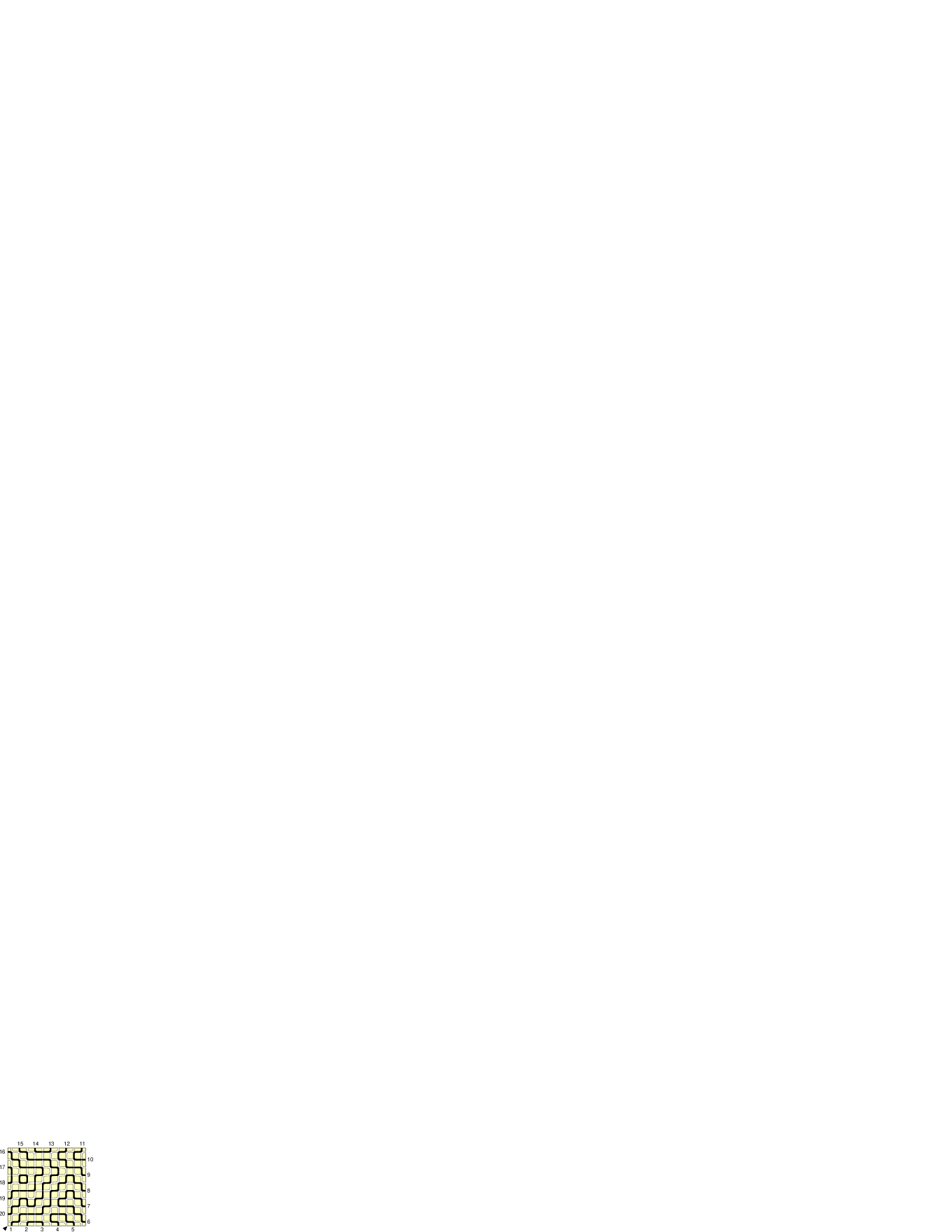
Figure 1: Comparison between the ‘ordinary’ map $\pi(\phi)$, on the left, and the ‘new’ map $\tilde{\pi}(\phi)$, on the right. Two distinct examples are shown in the two lines. In the first one, the refinement position is odd, $h(\phi)=5$, thus $\tilde{\pi}(\phi)$ is the appropriate rotation of the black link pattern of $\phi$. In the second line, $h(\phi)=4$, even, thus $\tilde{\pi}(\phi)$ is the appropriate rotation of the white link pattern of $\phi$.

We will then show how Di Francesco’s conjecture, now reducing to $\mathrm{Sym}\,\tilde{\Psi}_{\rm FPL}(t;\pi)=\mathrm{Sym}\,\Psi_{\rm FPL}(t;\pi)$, where $\mathrm{Sym}$ is a symmetrisation operator, follows from a study of the orbits under the action of Wieland half-gyration, and the associated evolution of the refinement position. Again, this is done for the general class of domains.

As already shown in [5], Di Francesco’s conjecture is a generalisation of the ordinary Razumov–Stroganov correspondence, thus this analysis also provides an alternative proof for the latter. However, there are various other alternative proofs that can be derived at various stages of the analysis. In particular, one derivation involves our sole Theorem 4.1, plus a non trivial bijection between $\mathpzc{Fpl}\!_{b}(\Lambda)$ and $\mathpzc{Fpl}\!_{+}(\Lambda)$, which preserves the link pattern associated to a configuration.

The paper is organized as follows. In Section 2 we introduce the Cyclic Temperley–Lieb Algebra, which is at the basis of the integrable structure of the $O(1)$ Dense Loop Model. In Section 2.2 we define the Temperley–Lieb Hamiltonian and the scattering equations, and derive some relevant properties of their solutions. In Section 3 we begin by recalling some basic facts about FPL’s, then we proceed with the definition of dihedral domains. In Section 3.3, we define the gyration operations acting on FPL, and show that they act as a rotation at the level of the link pattern associated to the FPL. This is the generalisation of the Wieland gyration theorem to our family of domains, and is essentially a reminder of the theory already presented in [3]. Sections 4 and 5 produce the results sketched above, in particular Theorem 4.1, stating that the ‘new’ FPL enumeration provides a solution of the scattering equation, and Theorem 5.1, the Di Francesco’s 2004 former conjecture, relating the ‘old’ and ‘new’ FPL enumerations.

2 The Cyclic Temperley–Lieb Algebra and the $O(1)$ Dense Loop Model

In this section we analyse the $O(1)$ Dense Loop Model side of the correpondence, which consists of the Perron–Frobenius eigenvector associated to the scattering equation, a linear equation involving a representation of the Temperley–Lieb Algebra. In Section 2.1 this algebra is defined, while in Section 2.2 we define our vector of interest, and deduce some of its properties.

2.1 The Cyclic Temperley–Lieb Algebra

We start by recalling the definiton of the Cyclic Temperley–Lieb Algebra $\mathrm{CTL}_{N}(\tau)$, which is the free algebra with generators $\{{\bf e}_{i}\}_{i\in\mathbb{Z}}$, and the invertible rotation operator $R$, and relations

$${\bf e}_{i} ={\bf e}_{i+N}\,; R^{\pm 1}{\bf e}_{i} ={\bf e}_{i\pm 1}R^{\pm 1}\,;$$ (3a)

$${\bf e}_{i}^{2} =\tau{\bf e}_{i}\,; {\bf e}_{i}{\bf e}_{i\pm 1}{\bf e}_{i} ={\bf e}_{i}\,;$$ (3b)

$$[{\bf e}_{i},{\bf e}_{j}] =0\makebox[0.0pt][l]{\rule{30.0pt}{0.0pt} {for $i-j\not\equiv\pm 1\ \ \mathrm{(mod\leavevmode\nobreak\ }N\mathrm{)}$.}}$$ (3c)

This algebra has interesting properties for a full range of the parameter $\tau$, and remarkable specialisation at a family of discrete values for $\tau$ (an useful alternative parametrisation is to set $\tau=-q-q^{-1}$). In the following we shall restrict to $\tau=1$, i.e. $q$ a cubic root of unity, and consider two kinds of diagrammatic representations of $\mathrm{CTL}_{N}(\tau)$, acting on spaces of link patterns.

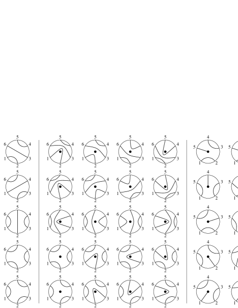
Figure 2: The sets $\mathpzc{LP}(6)$, $\mathpzc{LP}^{*}(6)$ and $\mathpzc{LP}^{*}(5)$.

Define $\mathpzc{LP}(2n)$ as the set whose elements are link patterns with $n$ arcs, i.e., the possible topologies of $n$ arcs that connect, through a non-crossing pairing, $2n$ points ordered cyclically counter-clockwise along the boundary of a disk. The set $\mathpzc{LP}^{*}(N)$ is an analogue of $\mathpzc{LP}(2n)$ consisting of punctured link patterns. For $N=2n$ even, these are the possible topologies of $n$ arcs that connect, through a non-crossing pairing, $2n$ points ordered cyclically along the boundary of a punctured disk (thus, it matters if an arc passes on the right or on the left of the punture). For $N=2n-1$ odd, these are the possible topologies of $n$ arcs that connect, through a non-crossing pairing, $2n-1$ points ordered cyclically along the boundary of a punctured disk, and the punture itself.

It is easily seen that the sets $\mathpzc{LP}(2n)$, $\mathpzc{LP}^{*}(2n)$ and $\mathpzc{LP}^{*}(2n+1)$ have cardinalities $C_{n}$, $(n+1)C_{n}$ and $(2n+1)C_{n}$, where $C_{n}=\frac{1}{n+1}\binom{2n}{n}$ is the $n$-th Catalan number. See Figure 2 for an illustration of these patterns.

It is useful to establish a reference pattern. We define a rainbow pattern as a link pattern consisting of a unique ‘rainbow’ of parallel arcs $\big{\{}\ldots,\{i,j\},\{i+1,j-1\},\{i+2,j-2\},\ldots\big{\}}$, with the possible puncture maximally nested. There are $n$ rainbow patterns in $\mathpzc{LP}(2n)$, and $N$ ones in $\mathpzc{LP}^{*}(N)$, related by rotation. Examples for $\mathpzc{LP}(8)$, $\mathpzc{LP}^{*}(8)$ and $\mathpzc{LP}^{*}(7)$ are

(4)

The first representation of $\mathrm{CTL}_{N}(\tau)$ we will consider is defined for $N=2n$ even, and acts on the vector space $\mathbb{C}^{\mathpzc{LP}(2n)}$, having a priviliged basis whose elements are indicised by elements of $\mathpzc{LP}(2n)$. The second class of representations acts on $\mathbb{C}^{\mathpzc{LP}^{*}(N)}$, with basis elements indicised by elements of $\mathpzc{LP}^{*}(N)$.

The action on the basis vectors is induced by the graphical action of the Temperley–Lieb generators on the link patterns. The operators ${\bf e}_{j}$ and $R$  are represented as customarily as

$${\bf e}_{j}:\quad \scriptstyle{N} \scriptstyle{1} \scriptstyle{2} \scriptstyle{\ldots} \scriptstyle{N} \scriptstyle{1} \scriptstyle{2\ldots} \scriptstyle{\ldots} \scriptstyle{j+1} \scriptstyle{j} \scriptstyle{j+1} \scriptstyle{j} R:\quad \scriptstyle{N} \scriptstyle{1} \scriptstyle{2} \scriptstyle{\ldots} \scriptstyle{N} \scriptstyle{1} \scriptstyle{2\ldots} \scriptstyle{\ldots}$$ (5)

Then, the action corresponds to the concatenation of the diagrams (an annulus, corresponding to an operator, is juxtaposed outside a disk, containing a link pattern, and a new pattern is derived from the topology of the matching of the new boundary points). In case loops are produced, they are dropped, with a factor $\tau$ each (i.e., in our specialisation to $\tau=1$, we just forget about loops).

It is easily seen that the representation on $\mathpzc{LP}(2n)$ is a quotient of the representation on $\mathpzc{LP}^{*}(2n)$, obtained by just ‘forgetting’ about the location of the puncture.

For two terminations $i,j\in\{1,\ldots,N\}$, and a link pattern $\pi$, we write that $i\sim j$ if $(ij)$ is an arc of $\pi$, and $i\nsim j$ otherwise. If the terminations are consecutive, we say that $i\includegraphics{fig_sim.eps}i+1$ if $\pi$ is in the image of $e_{i}$, and $i\includegraphics{fig_nsim.eps}i+1$ otherwise. In $\mathpzc{LP}(2n)$ and $\mathpzc{LP}^{*}(2n+1)$, $i\includegraphics{fig_sim.eps}i+1$ if and only if $i\sim i+1$, while in $\mathpzc{LP}^{*}(2n)$, $i\includegraphics{fig_sim.eps}i+1$ if and only if $i\sim i+1$ and this short arc does not embrace the puncture.

Working in the linear spaces $\mathbb{C}^{\mathpzc{LP}(2n)}$ and $\mathbb{C}^{\mathpzc{LP}^{*}(N)}$ we use a “ket” notation for vectors $\mbox{$|v\rangle$}=\sum_{\pi}v(\pi)\mbox{$|\pi\rangle$}$, with the sum over $\pi$ running in the appropriate ensemble $\mathpzc{LP}(2n)$ or $\mathpzc{LP}^{*}(N)$ depending on circumstances. We denote covectors as $\langle v|$, and scalar products $\sum_{\pi}u(\pi)^{*}v(\pi)$ as $\big{\langle}u|v\big{\rangle}$ (in fact, complex conjugation is never used here, and we could have worked equivalently in the linear spaces $\mathbb{R}^{\mathpzc{LP}(2n)}$ or $\mathbb{Q}^{\mathpzc{LP}(2n)}$). Such a notation is chosen in order to distinguish easily vectors, linear operators and covectors, while omitting the specification of the space, between $\mathbb{C}^{\mathpzc{LP}(2n)}$ and $\mathbb{C}^{\mathpzc{LP}^{*}(N)}$, writing single equations that hold simultaneously in the two cases. The maps ${\bf e}_{i}$ and $R$ induce linear operators on $\mathbb{C}^{\mathpzc{LP}(2n)}$ and $\mathbb{C}^{\mathpzc{LP}^{*}(N)}$, for which, with abuse of notation, we continue to use the same symbols.

2.2 The Hamiltonian, the scattering matrix and the scattering equations

Consider a special linear expression in Temperley–Lieb Algebra, named Hamiltonian

$$H_{0}=\sum_{i=1}^{N}({\bf e}_{i}-{\bf 1})\,.$$ (6)

The action of this operator, both on $\mathbb{C}^{\mathpzc{LP}(2n)}$ (if $N=2n$) and on $\mathbb{C}^{\mathpzc{LP}^{*}(N)}$, has at sight a unique left null-vector, $\mbox{$\langle 1|$}=\sum_{\pi}\mbox{$\langle\pi|$}$. The ground state of the Hamiltonian is the unique right null-vector, i.e. the unique vector $\mbox{$|\Psi_{O(1)}\rangle$}\in\mathbb{C}^{\mathpzc{LP}(2n)}$ (or in $\mathbb{C}^{\mathpzc{LP}^{*}(N)}$) satisfying

$$H_{0}\mbox{$|\Psi_{O(1)}\rangle$}=0\,.$$ (7)

In this section we omit the $O(1)$ subscript for brevity. The vector $|\Psi\rangle$ can clearly be normalised in such a way that all of its entries are integers (because $H_{0}$ has integer entries). Furthermore, all the entries are positive. This comes from the stochastic nature of $H_{0}$ (i.e., $|\Psi\rangle$ is the Perron–Frobenius vector for the matrix $\frac{1}{N}H_{0}+{\bf 1}$).

Following closely [5], we now introduce a family of equations, called scattering equations, depending on one parameter $t$, that generalise (7), in the sense that the solutions $|\Psi^{(i)}(t)\rangle$ of the $i$-th equation at parameter $t$ reduce to the ground state $|\Psi\rangle$ of the Hamiltonian, when $t=1$. Introduce the operator $X_{i}(t)$ 

$$X_{i}(t)=t\;{\bf 1}+(1-t)\,{\bf e}_{i}\,.$$ (8)

The scattering equation we are going to consider is

$$X_{i}(t)\mbox{$|\Psi^{(i)}(t)\rangle$}=R\,\mbox{$|\Psi^{(i)}(t)\rangle$}\,.$$ (9)

A simple analysis of equation (9) tells us that its solution is unique up to normalization. Indeed, if $0<t<1$, the matrix $R\,X_{i}(t)$ is a Markov chain and it is not difficult to show that it is irreducible. Therefore existence and unicity (up to normalization) of the solution of equation (9) follow from the Perron–Frobenius theorem, in a way completely analogous to the reasoning done for $|\Psi\rangle$ and the Hamiltonian. The components $\Psi^{(i)}(t;\pi)$ of the vector $|\Psi^{(i)}(t)\rangle$ can be normalized in such a way that they are polynomials of the parameter $t$ and the Perron–Frobenius theorem ensures their positivity, when evaluated on the open real interval $t\in\;]0,1[$, but remarkably not the observed, and proven later on, coefficient-wise positivity.

In general $|\Psi^{(i)}(t)\rangle$ is not dihedrally invariant (as we will see later on, it is only “dihedrally covariant”, for a simultaneous action on link patterns $\pi$ and superscript $(i)$). The dihedral symmetry is however restored at $t=1$, where $|\Psi^{(i)}(t)\rangle$ reduces to the solution of equation (7). Indeed, for $t\to 1$, the operators $X_{i}(t)$ reduce to the identity, and therefore from equation (9) it follows immediately that $|\Psi^{(i)}(1)\rangle$ is rotationally invariant

$$\mbox{$|\Psi^{(i)}(1)\rangle$}=R\,\mbox{$|\Psi^{(i)}(1)\rangle$}\,.$$ (10)

Furthermore, if we apply the projector

$$\mathrm{Sym}:=\frac{1}{N}\sum_{i=0}^{N-1}R^{k}$$ (11)

on both sides of equation (9) (and use the obvious $\mathrm{Sym}\,R=\mathrm{Sym}$) we find

$$\mathrm{Sym}\,({\bf e}_{i}-{\bf 1})\mbox{$|\Psi^{(i)}(t)\rangle$}=0\,.$$ (12)

Combining equations (10) and (12), we obtain

$$\begin{split}H_{0}\mbox{$|\Psi^{(i)}(1)\rangle$}&=\sum_{k=0}^{N-1}R^{k}({\bf e}_{i}-{\bf 1})R^{-k}\mbox{$|\Psi^{(i)}(1)\rangle$}=\sum_{k=0}^{N-1}R^{k}({\bf e}_{i}-{\bf 1})\mbox{$|\Psi^{(i)}(1)\rangle$}\\ &=N\,\mathrm{Sym}\,({\bf e}_{i}-{\bf 1})\mbox{$|\Psi^{(i)}(1)\rangle$}=0\,;\end{split}$$ (13)

i.e., $|\Psi^{(i)}(1)\rangle$ is proportional to the ground state of the Hamiltonian. An alternate derivation of the same result, already presented in [5], goes through the definition of the scattering matrix

$$S_{i}(t)=X_{i+N-1}(t)\cdots X_{i+1}(t)X_{i}(t)\,.$$ (14)

Since $R^{k}X_{i}(t)R^{-k}=X_{i+k}(t)$, we find that

$$X_{i+k}(t)X_{i+k-1}(t)\dots X_{i+1}(t)X_{i}(t)=R^{k+1}(R^{-1}X_{i}(t))^{k+1}\,,$$ (15)

and therefore, if $\Psi^{(i)}(t)$ satisfies equation (9), then it must satisfy

$$X_{i+k}(t)X_{i+k-1}(t)\dots X_{i+1}(t)X_{i}(t)\mbox{$|\Psi^{(i)}(t)\rangle$}=R^{-k-1}\mbox{$|\Psi^{(i)}(t)\rangle$}\,,$$ (16)

and in particular

$$\big{(}S_{i}(t)-{\bf 1}\big{)}\mbox{$|\Psi^{(i)}(t)\rangle$}=0\,.$$ (17)

Observe that, for all $i$, the expansion of $S_{i}(t)$ near $t=1$ leads to the Hamiltonian. Indeed $S_{i}(1)={\bf 1}$, and

$$\left.\frac{dS_{i}(t)}{dt}\right|_{t=1} =\sum_{j=i}^{i+N-1}\left.X_{i+N-1}(t)\cdots X_{j+1}(t)\frac{dX_{j}(t)}{dt}X_{j-1}(t)\cdots X_{i}(t)\right|_{t=1}=-H_{0}\,;$$ (18)

therefore, taking the derivative of equation (17) and then setting $t=1$, one finds that $\Psi^{(i)}(1)$ satisfies equation (7).

As anticipated, the solutions of equation (9) show dihedral covariance for different values of $i$. Indeed we find that

$$0=\big{(}X_{i}(t)-R\big{)}\,\mbox{$|\Psi^{(i)}(t)\rangle$}=R^{-1}\big{(}X_{i+1}(t)-R\big{)}R\,\mbox{$|\Psi^{(i)}(t)\rangle$}\,,$$ (19)

that is,

$$\mbox{$|\Psi^{(i+1)}(t)\rangle$}=R\,\mbox{$|\Psi^{(i)}(t)\rangle$}$$ (20)

(more precisely, our reasoning only proves that $\mbox{$|\Psi^{(i+1)}(t)\rangle$}\propto R\,\mbox{$|\Psi^{(i)}(t)\rangle$}$, however, as all the components are real-positive for $0<t<1$, and $\mbox{$|\Psi^{(i+N)}(t)\rangle$}\equiv\mbox{$|\Psi^{(i)}(t)\rangle$}$, the proportionality factor must be 1).

Call $V$ the operator that applies a vertical symmetry to $\pi$, i.e., if $\{i,j\}$ is an arc of $\pi$, $\{N+1-j,N+1-i\}$ is an arc of $V\pi$. Clearly,

$$V^{2} ={\bf 1}\,; VR^{\pm 1}V =R^{\mp 1}\,; V{\bf e}_{i}V ={\bf e}_{N-i}\,.$$ (21)

Then, as $X_{i}(t)^{-1}=X_{i}(t^{-1})$,

$$\begin{split}0&=\big{(}X_{i}(t)-R\big{)}\,\mbox{$|\Psi^{(i)}(t)\rangle$}=X_{i}(t)\big{(}R^{-1}-X_{i}(t^{-1})\big{)}R\,\mbox{$|\Psi^{(i)}(t)\rangle$}\\ &=-X_{i}(t)V\big{(}X_{N-i}(t^{-1})-R\big{)}VR\,\mbox{$|\Psi^{(i)}(t)\rangle$}\,,\end{split}$$ (22)

that is, $\mbox{$|\Psi^{(N-i)}(t^{-1})\rangle$}\propto VR\,\mbox{$|\Psi^{(i)}(t)\rangle$}$, or, using (20),

$$\mbox{$|\Psi^{(i)}(t^{-1})\rangle$}\propto V\,\mbox{$|\Psi^{(N+1-i)}(t)\rangle$}\,.$$ (23)

In fact the proportionality factor is $t^{-(n-1)}$ for the case $\mathpzc{LP}(2n)$, and $t^{-(N-1)}$ for the case $\mathpzc{LP}^{*}(N)$, but this will only be determined from the following Proposition 4.1. Note that equation (23) corresponds to Claim 3 in [5]. Also note that the covariance under vertical reflection implies that our collection of solutions $|\Psi^{(i)}(t)\rangle$ of the scattering equations (9) are related to the solutions of the modified version in which the other direction of rotation is considered, $X_{i}(t)\mbox{$|\Psi\rangle$}=R^{-1}\mbox{$|\Psi\rangle$}$.

At the light of the dihedral covariance discussed above, we can concentrate on the case $i=1$ without loss of generality. All the results that follow can be easily translated to arbitrary values of $i$. For short, call $\Psi(t)$ the vector $\Psi^{(1)}(t)$.

As ${\bf e}_{1}^{2}={\bf e}_{1}$, the operators ${\bf e}_{1}$ and $({\bf 1}-{\bf e}_{1})$ are orthogonal projectors, and a vector satisfies equation (9) if and only if it satisfies the system of linear equations associated to these two projectors

$${\bf e}_{1}\big{(}t{\bf 1}-R-(t-1){\bf e}_{1}\big{)}\mbox{$|\Psi(t)\rangle$} =0\,;$$ (24)

$$(1-{\bf e}_{1})\big{(}t{\bf 1}-R-(t-1){\bf e}_{1}\big{)}\mbox{$|\Psi(t)\rangle$} =0\,.$$ (25)

Applying the rules of Temperley–Lieb Algebra leads to

$${\bf e}_{1}({\bf 1}-R)\mbox{$|\Psi(t)\rangle$} =0\,;$$ (26)

$$({\bf 1}-{\bf e}_{1})\big{(}t{\bf 1}-R\big{)}\mbox{$|\Psi(t)\rangle$} =0\,.$$ (27)

The first equation has the simplifying property of involving an operator independent of $t$. The second equation is better investigated in components

$$\begin{split}(1-{\bf e}_{1})\big{(}t{\bf 1}-R\big{)}\mbox{$|\Psi(t)\rangle$}&=(1-{\bf e}_{1})\Big{(}\sum_{\pi}t\Psi(t;\pi)\mbox{$|\pi\rangle$}-\sum_{\pi}\Psi(t;\pi)\mbox{$|R\pi\rangle$}\Big{)}\\ &=(1-{\bf e}_{1})\Big{(}\sum_{\pi}t\Psi(t;\pi)\mbox{$|\pi\rangle$}-\sum_{\pi}\Psi(t;R^{-1}\pi)\mbox{$|\pi\rangle$}\Big{)}\\ &=\sum_{\pi}\big{(}t\Psi(t;\pi)-\Psi(t;R^{-1}\pi)\big{)}(1-{\bf e}_{1})\mbox{$|\pi\rangle$}\,.\end{split}$$ (28)

In this sum, a component $\pi$ with $1\includegraphics{fig_sim.eps}2$ is annihilated by $1-{\bf e}_{1}$. For (27) to hold, as a component $\pi$ with $1\includegraphics{fig_nsim.eps}2$ has coefficient $t\Psi(t;\pi)-\Psi(t;R^{-1}\pi)$, this must be zero. For later reference we record the previous observations as a proposition.

Proposition 2.1.

A necessary and sufficient condition for $|\Psi(t)\rangle$ to solve the scattering equation at $i=1$, equation (9), is that

$${\bf e}_{1}({\bf 1}-R)\mbox{$|\Psi(t)\rangle$} =0\,;$$ (29)

and that, for any component $\pi$ such that $1\includegraphics{fig_nsim.eps}2$,

$$t\,\Psi(t;\pi) =\Psi(t;R^{-1}\pi)\,.$$ (30)

This proposition will be employed in Section 4, in the proof of Theorem 4.1. However, already at this point it is useful for deducing a corollary of some importance.

Corollary 2.1.

All the polynomial solutions $\Psi(t;\pi)$ of the scattering equation have degree at least $n-1$ in the case $\mathpzc{LP}(2n)$, and at least $N-1$ in the case $\mathpzc{LP}^{*}(N)$.

This comes from investigating the consequences on rainbow patterns of equation (30) in Proposition 2.1,

There are various possible derivations of the fact that a normalisation of the solution exists such that the degree is exactly the one given above. In particular, one proof will follow later on from our analysis (see Proposition 4.1).

2.3 Further properties of the ground state

This section discusses some other properties of the ground states $\Psi$ and $\Psi^{(i)}(t)$, that are not strictly necessary in the derivation of the results of this paper, but are of interest in the combinatorial connection with enumerations of FPLs, and allow to understand some of the implications of our results.

As we stated above, it follows from the stochasticity of the Hamiltonian and of the scattering matrix, the fact that the defining equations involve integer coefficients, and from the Perron–Frobenius theorem, that the components $\Psi(\pi)$ can be normalised to be positive integers, and the components $\Psi^{(i)}(t;\pi)$ can be normalised to be integer-valued polynomials in $t$, everywhere positive in the open interval $t\in\;]0,1[$.

Much more than this is true. The components $\Psi(\pi)$ can be normalised to ‘small’ integers, in particular they remain all integers if the entry of smallest component, corresponding to the rainbow pattern, is set to 1. Furthermore, the components $\Psi^{(i)}(t;\pi)$ can be normalised to be integer-valued polynomials in $t$, with all positive coefficients, and in such a way that the coefficients are still integers, when the entries of the various rainbow patterns (for the various rotations) are set to monomials $t^{j}$. This means in particular that the smallest normalisation that makes the $\Psi(\pi)$’s all integers, and the smallest normalisation that makes the $\Psi^{(i)}(t;\pi)$’s all integer-valued polynomials, are such that $\Psi^{(i)}(t;\pi)|_{t=1}=\Psi(\pi)$, without proportionality factors. Finally, with this normalisation of the solution, the maximum degree in the collections of polynomials coincides with the lower bounds given in Corollary 2.1.

All of the claims of the previous paragraph follow from the Razumov–Stroganov correspondence, either in its original form (for the claims concerning $\Psi(\pi)$) or in the refined version discussed here (for the claims concerning $\Psi^{(i)}(t;\pi)$), through the interpretation of the ground state components as enumerations of FPL’s. Some of the claims have alternative, purely algebraic proofs, which are mostly based on the observation that the vectors $|\Psi^{(i)}(t)\rangle$ are a special case of $|\Psi(z_{1},\dots,z_{N})\rangle$, the ground state of the fully inhomegenous $O(1)$ Dense Loop Model. More precisely,

$$\mbox{$|\Psi^{(i)}(t)\rangle$}\propto\mbox{$|\Psi\big{(}1,\ldots,1,z_{i}=\genfrac{}{}{0.25pt}{1}{qt+q^{-1}}{q+q^{-1}t},1,\ldots,1\big{)}\rangle$}\,.$$ (31)

The claim on the degree in $t$ can be deduced by the analogous claim on the degree in the $z_{i}$’s, provided in [6] for the $\mathpzc{LP}(2n)$ case, and in [7] for the $\mathpzc{LP}^{*}(N)$ case. As a byproduct, one also obtains the fact that rainbow pattern components are of the form $t^{j}$. Furthermore, also the claim on the integrality of the components $\Psi(\pi)$ can be proven (see e.g. [17, sec. 4.4]).

We have seen that, for $t=1$, the ground states of the scattering matrix, $\Psi^{(i)}(t;\pi)$, reduce to the one of the Hamiltonian. Another interesting specialization is $t=0$ (or its symmetric $t\to\infty$). From equation (30) in Proposition 2.1, in this limit $|\Psi_{N}^{(i)}(0)\rangle$ lies in the image of ${\bf e}_{i-1}$, i.e., for $\pi\in\mathpzc{LP}(N)$ (or $\mathpzc{LP}^{*}(N)$), $\Psi_{N}^{(i)}(0,\pi)=0$ if $i-1\includegraphics{fig_nsim.eps}i$ in $\pi$. This subset of link patterns is in natural correspondence with the full set $\mathpzc{LP}(N-2)$ (or $\mathpzc{LP}^{*}(N-2)$), upon removing the short arc between $i-1$ and $i$. As a consequence of a recursion relation satisfied by $|\Psi(z_{1},\dots,z_{N})\rangle$ and proven in [6] (Theorem 3), this specialisation and correspondence produces a vector that satisfies equation (7) at size $N-2$. The solution of this equation with non-negative entries is unique, and the customary fixing of the normalisation, e.g. for the rainbow pattern containing the arc $\{i-1,i\}$, allows to fix the proportionality factor to 1:

$$\Psi_{N}^{(i)}\Big{(}0,\begin{picture}(8.0,2.8)\put(0.0,0.0){\includegraphics[scale={1.2}]{fig_LP_iim1.eps}} \put(2.2,-1.0){${}_{i-1}\;{}_{i}$} \put(1.8,0.8){$\pi$} \end{picture}\Big{)}=\Psi_{N-2}^{(i)}(1,\pi)\,.$$ (32)

3 Fully-packed loops

In this section we present the relevant facts on Fully-Packed Loops that we will need in the proofs of our results. Section 3.1 presents the main definitions. Section 3.2 introduces a family of domains, that we call dihedral domains, for which our theorems do hold. These domains have a common behaviour under gyration, a bijection introduced by Wieland [14] for FPL’s in the square. This operation is analysed in detail in Section 3.3.

3.1 Fully-packed loops: basic definitions

Consider a graph $\Lambda$ in which all the vertices have degree in the set $\{1,2,4\}$. If the degree is 2 or 4, we say that the vertex is internal, while if the degree is 1 we say that the vertex is external, and that the incident edge is an external edge. Obvious parity reasons force to have an even number of external edges.

We say that $\Lambda$ is outer-planar if it admits a planar embedding into a disk, with all the external vertices on the boundary of the disk. Such an embedding defines univocally the faces of the domain, and induces a cyclic ordering of the external vertices and edges.

We will be interested in maps $\phi:E(\Lambda)\to\{b,w\}$, naturally identified with bicolourations of the edge-set of the graph (and $b$, $w$ stand for black, white). The map $\phi$ is a fully-packed loop (FPL) configuration if all the internal vertices of degree 4 have two black and two white adjacent edges, and all the vertices of degree 2 have one black and one white adjacent edge. The map $\phi$ has boundary condition $\tau$ if its restriction to the external edges is $\tau$. We define $\mathpzc{Fpl}\!(\Lambda;\tau)$ the set of FPL’s on $\Lambda$, with boundary condition $\tau$. We call $\overline{\tau}$ the boundary condition with black and white exchanged. For $\phi\in\mathpzc{Fpl}\!(\Lambda;\tau)$, the conjugate configuration $\sigma(\phi)\in\mathpzc{Fpl}\!(\Lambda;\overline{\tau})$ is the one obtained interchanging black and white. If $\Lambda$ is outer-planar, there are two specially important boundary conditions, $\tau_{+}=(b,w,b,w,\ldots,b,w)$ and $\tau_{-}=\overline{\tau_{+}}=(w,b,w,b,\ldots,w,b)$, that we call alternating boundary conditions. We also use the shortcuts $\mathpzc{Fpl}\!_{+}(\Lambda)=\mathpzc{Fpl}\!(\Lambda;\tau_{+})$ and $\mathpzc{Fpl}\!_{-}(\Lambda)=\mathpzc{Fpl}\!(\Lambda;\tau_{-})$.

The black and the white edges of $\phi$, separately, form a collection of cycles and of open paths with endpoints at vertices of degree $1$ or $2$. The open paths of each given colouration connect external vertices and internal vertices of degree $2$ among themselves, thus inducing two pairings, $\pi_{b}$ and $\pi_{w}$ for black and white respectively, and two integers, $\ell_{b}$ and $\ell_{w}$, for the number of black and white cycles in $\phi$. Call $\ell=\ell_{b}+\ell_{w}$.

If $\Lambda$ is outer-planar, and has no vertices of degree 2, and $\tau$ has $2n_{b}$ black and $2n_{w}$ white entries, $\pi_{b}$ and $\pi_{w}$ are link patterns in $\mathpzc{LP}(2n_{b})$ and $\mathpzc{LP}(2n_{w})$, i.e. they have no crossings. If $\Lambda$ has a marked face, $\pi_{b}$ and $\pi_{w}$ are punctured link patterns in $\mathpzc{LP}^{*}(2n_{b})$ and in $\mathpzc{LP}^{*}(2n_{w})$, with the puncture located inside the marked face. If it has exactly one vertex of degree 2, and $\tau$ has $2n_{b}-1$ black and $2n_{w}-1$ white entries, $\pi_{b}$ and $\pi_{w}$ are punctured link patterns in $\mathpzc{LP}^{*}(2n_{b}-1)$ and $\mathpzc{LP}^{*}(2n_{w}-1)$, with the puncture located at this vertex.

The case corresponding to the original Razumov–Stroganov correspondence is the one in which $\Lambda$ is a square $n\times n$ grid, with $n^{2}$ internal vertices of degree 4, and $4n$ external vertices, adjacent to the internal vertices in the obvious way. Note that, for $n$ sufficiently large, the outer-planar embedding is unique, up to reflection symmetry, and to permutation of the pairs of external edges adjacent to corners.

3.2 Dihedral domains: definition and properties

A tool in the combinatorial investigation of FPL’s, started with the work of Wieland [14], is that on the $n\times n$ square with alternating boundary conditions there exist two bijections $H_{\pm}$ between $\mathpzc{Fpl}\!_{+}(\Lambda)$ and $\mathpzc{Fpl}\!_{-}(\Lambda)$, that preserve the link pattern up to a rotation, which imply relations between the enumerations of FPL’s with a given triple $(\pi_{b},\pi_{w},\ell)$.

This property of the maps $H_{\pm}$ has been crucial for the proof of the Razumov–Stroganov correspondence in [3], where it was mentioned that analogues of the maps $H_{\pm}$ exist on a more general class of outer-planar domains characterized by the following two properties:

• the internal faces have at most $4$ sides,

• the faces formed by joining two consecutives external edges have at most $3$ sides.

In the present paper we exhibit a family of graphs, that we call dihedral domains, that satisfy these properties. All our results holds on this class of domains.

In [4] we shall perform a classification of all the domains presenting a version of the Wieland Theorem, without any a priori assumption (for example, without assuming outer-planarity).

We produce two families of dihedral domains. Domains of the first kind present the version of the Razumov–Stroganov correspondence on $\mathpzc{LP}(2n)$ and, in certain circumstances, also the more refined version on $\mathpzc{LP}^{*}(2n)$. Domains of the second kind present the version of the correspondence on $\mathpzc{LP}^{*}(2n-1)$.

      

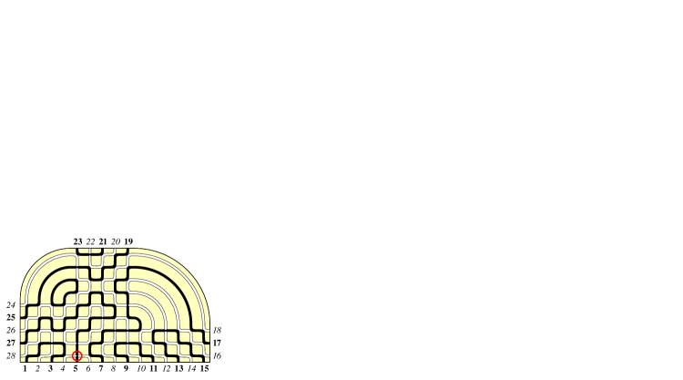
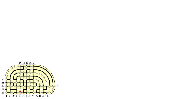
Figure 3: Typical domains $\Lambda$, with two corners (left) and one corner (right), together with a configuration $\phi\in\mathpzc{Fpl}\!_{+}(\Lambda)$. The domain on the left is $\Lambda(15,9;0,0,6,4)$, and has $2n=14$ and $L=15$. The domain on the right is $\Lambda(15,9;0,2,6,4)$, and has $2n=12$ and $L=24$. In both cases, $h(\phi)=5$, because on the reference line the position of the only $c$-type tile is adjacent to the 5-th external edge.

A domain of the first kind has six integer parameters, $\Lambda=\Lambda(L_{x},L_{y};a_{1},a_{2},a_{3},a_{4})$. Take a rectangular $L_{x}\times L_{y}$ portion of the square grid, and call $A_{1},\ldots,A_{4}$ the four corners, in counter-clockwise order starting from the bottom-left one. From the corner $A_{i}$, cut away an $a_{i}\times a_{i}$ square portion of the grid. The parameters must be such that the removed squares do not overlap, although they might share a portion of the perimeter (e.g., $a_{1}+a_{2}=L_{x}$ is admitted, but $a_{1}+a_{2}=L_{x}+1$ is not). Each removed square will cut $2a_{i}$ internal edges, which are connected pairwise, starting from the resulting concave angle. The number of external edges is $2(L_{x}+L_{y}-a_{1}-a_{2}-a_{3}-a_{4})$, and the parameter $2n$ of the set of link patterns will be given by

$$2n=L_{x}+L_{y}-a_{1}-a_{2}-a_{3}-a_{4}\,.$$ (33)

Domains defined by this procedure have all faces with at most $4$ sides. They are constituted of a finite number of bundles of parallel lines (at least 2 and at most 6 bundles), that cross each other forming portions of the square grid. These lines are the geometric structures to which, in the general framework of the integrable 6-Vertex Model, are associated spectral parameters. One line is a boundary line if it is adjacent to some external edges.

Define a corner as a vertex adjacent to two external edges, and call $c_{\Lambda}$ the number of corners in $\Lambda$, which also coincides with the number of boundary lines. For a face with $\ell$ sides, the curvature of the face is $4-\ell$. The total curvature of the domain, $d_{\Lambda}$, is the sum of the curvatures of all the faces. The number of corners $c_{\Lambda}$ is exactly $4$ minus the number of non-zero $a_{i}$’s, and is related to the total curvature by an Euler formula, $c_{\Lambda}=4-d_{\Lambda}$. Examples of dihedral domains with $c_{\Lambda}=2$ and $c_{\Lambda}=1$ are shown in Figure 3, together with examples of FPL.

      

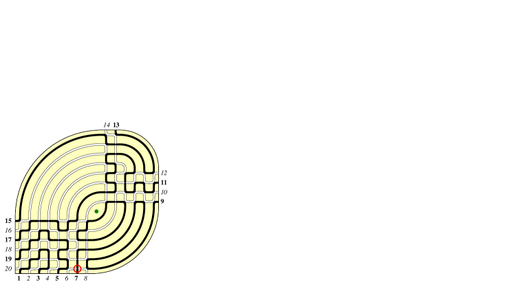
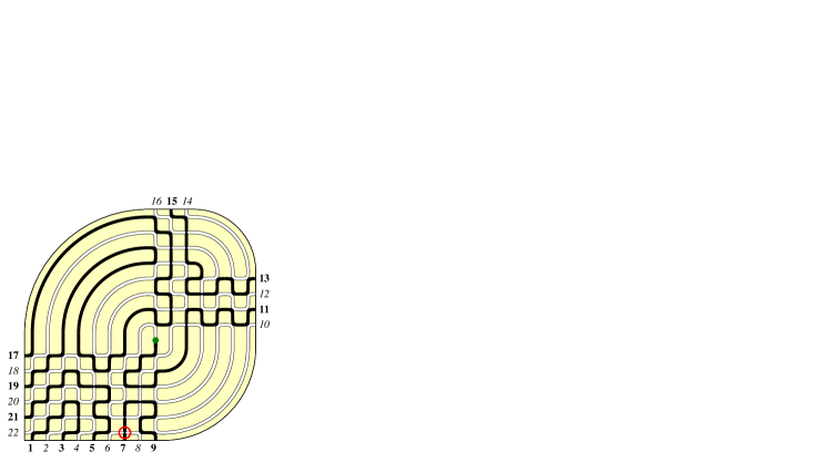
Figure 4: Left: a typical domain $\Lambda$ of the first kind, with one face of two sides, showing Razumov–Stroganov correspondence for punctured link patterns $\mathpzc{LP}^{*}(2n)$. This domain is $\Lambda(14,14;0,6,4,8)$, and has $2n=10$ and $L=20$. It has one face with two sides because $L_{x}=L_{y}=a_{2}+a_{4}$. Right: a typical domain $\Lambda$ of the second kind, with one vertex of degree 2, showing Razumov–Stroganov correspondence for punctured link patterns $\mathpzc{LP}^{*}(2n-1)$. This domain is $\Lambda(15,14;0,6,4,8)$, and has $2n-1=11$ and $L=22$. It allows for a vertex of degree 2, because $L_{x}-1=L_{y}=a_{2}+a_{4}$. The puncture is marked in green. Typical configurations $\phi\in\mathpzc{Fpl}\!_{+}(\Lambda)$ are shown. both with $h(\phi)=7$.

As domains with $c_{\Lambda}=0$ have refined enumerations of FPL’s which are easily related to the ones of a reduced domain, in the following we restrict to the ‘irreducible’ case in which there is at least one corner (thus $c_{\Lambda}\geq 1$, or equivalently $d_{\Lambda}\leq 3$).

Because of the rotational invariance of the parameter space, we can set $a_{1}=0$ without loss of generality, and set the corner $A_{1}$ as the reference corner of the domain. The external edges are labeled in counter-clockwise order, starting from this corner, and the reference side of the domain is the boundary line adjacent to the external edges with labels $1,2,\ldots,$ up to when another corner is reached. We will call $L$ the length of the reference side, i.e. the number of vertices along this side. The dependence of $L$ from our parameters depends on which corners are present, as $L=L_{x}$ if $a_{2}=0$, $L=L_{x}+L_{y}-2a_{2}$ if $a_{2}>0$ and $a_{3}=0$, and so on.

Under the restriction to $c_{\Lambda}\geq 1$, our domains have at most one face with $1$ or $2$ sides. The set of domains with one such face coincides with the set of domains that allow for the $\mathpzc{LP}^{*}(2n)$ version of the Razumov–Stroganov correspondence, and the puncture is located inside this special face. A dihedral domain of this type, together with a FPL configuration, is shown in Figure 4, left.

Dihedral domains of the second kind are a variant of a subclass of domains of the first kind, that have an internal edge $e$ for which both adjacent faces have at most 3 sides. This edge is splitted in two, and a vertex of degree $2$ is produced. Note that, after this procedure, still the adjacent faces have at most 4 sides, as required. Note also that, again by reasonings of curvature, this procedure cannot be applied more than once (indeed, in the Euler formula, a vertex of degree $4-d$ carries $d$ units of curvature). The parameter $2n-1$ of the set of link patterns $\mathpzc{LP}^{*}(2n-1)$ is given by

$$2n-1=L_{x}+L_{y}-a_{1}-a_{2}-a_{3}-a_{4}\,,$$ (34)

and the puncture of the link patterns is located at the vertex of degree 2. A dihedral domain of second kind, together with a FPL configuration, is shown in Figure 4, right.

Given a dihedral domain $\Lambda$, we will be interested in the set $\mathpzc{Fpl}\!(\Lambda)$ of FPL configurations with alternating boundary conditions. Depending on the parity of the labels of the external black edges, the set $\mathpzc{Fpl}\!(\Lambda)$ splits in two equinumerous subsets, $\mathpzc{Fpl}\!_{+}(\Lambda)$ and $\mathpzc{Fpl}\!_{-}(\Lambda)$, which contains FPL such that the external edge with label 1 is black or white. The operation $\sigma$, which consists in inverting the colouration of all the edges, is an involution in $\mathpzc{Fpl}\!(\Lambda)$, which provides a trivial bijection between $\mathpzc{Fpl}\!_{+}(\Lambda)$ and $\mathpzc{Fpl}\!_{-}(\Lambda)$.

We recall that at every vertex of degree 4, given an ordering of the two crossing lines, there are 6 possible local configurations (this is the origin of the name “6-Vertex Model”), pairwise related by the involution $\sigma$

(35)

We will say that a FPL $\phi$ has a tile of type $a$, $b$ or $c$ at a given vertex of degree-4, when the ordering of the two lines is unambiguous. This is in particular the case for vertices adjacent to an external line.

It is easy to see that, because of the alternating boundary conditions, each $\phi\in\mathpzc{Fpl}\!(\Lambda)$ is forced to have a single $c$-tile on any of the boundary sides, with all $a$-tiles and $b$-tiles along the line, at the right and the left of the $c$-tile, respectively. In particular, there is a single $c$-tile at position $1\leq h(\phi)\leq L$ along the reference side. We call $h(\phi)$ the refinement position of the FPL $\phi$ (it is understood, w.r.t. the reference side).

We call $\mathpzc{Fpl}\!_{b}(\Lambda)$ and $\mathpzc{Fpl}\!_{w}(\Lambda)$ the subsets of $\mathpzc{Fpl}\!(\Lambda)$ consisting of FPL such that the edge incident to the refinement position is black or white. The operation $\sigma$ is also trivially a bijection between $\mathpzc{Fpl}\!_{b}(\Lambda)$ and $\mathpzc{Fpl}\!_{w}(\Lambda)$.

For a dihedral domain $\Lambda$, we will denote with $\mathpzc{LP}(\Lambda)$ the set $\mathpzc{LP}(2n)$, $\mathpzc{LP}^{*}(2n)$ or $\mathpzc{LP}^{*}(2n-1)$, depending from the kind of domain, and for the appropriate value of $n$. The only ambiguity holds for those domains of the first kind for which both the $\mathpzc{LP}(2n)$ and the $\mathpzc{LP}^{*}(2n)$ correspondences are viable. As the latter is a stronger version of the former, we can assume without loss of generality that $\mathpzc{LP}(\Lambda)=\mathpzc{LP}^{*}(2n)$ in such a case.

Figure 5: Dihedral domains associated to symmetry classes of ASM that present dihedral Razumov–Stroganov correspondence. Top-left and top-right: HTASM of even and odd size, respectively; bottom-left: QTASM of size $4n$; bottom-right: quasi-QTASM of size $4n+2$. In the link patterns, the notation $i\,(j)$ stands for the fact that the link pattern termination is the image on the FPL of an external edge, which is the $i$-th one counting from the refinement position, and of the colour of the refinement position, and the $j$-th one (including both colourings) counting from the reference corner.

We conclude the present section by observing that some particular dihedral domains correspond to symmetry classes of FPL’s (and thus of Alternating Sign Matrices) that have been already studied in the literature (see [11], and [8] for quasi-QTASM). Figure 5 gives illustrations of these classes.

ASM:

When all $a_{i}$ are zero, and $L_{x}=L_{y}$, the domain is the square, and the FPLs are in bijection with all Alternating Sign Matrices. Note that conversely, when all $a_{i}$ are zero and $L_{x}\neq L_{y}$, $\mathpzc{Fpl}\!(\Lambda)=\varnothing$.

HTASM:

For any two of the $a_{i}$’s equal to 0, and the other two equal to $n$, and $L_{x}=L_{y}=2n$, we get Half-Turn Symmetric ASM (HTASM) of size $2n$, while for $a_{1}=a_{3}=0$, $a_{2}=a_{4}=n$ and $L_{x}-1=L_{y}=2n$, as we have an edge adjacent to two triangular faces, we can construct a dihedral domain of the second kind, which corresponds to HTASM of size $2n+1$ (see Figure 5, top).

QTASM:

For $a_{1}=0$, $a_{2}=a_{3}=a_{4}=2n$ and $L_{x}=L_{y}=4n$ we get Quarter-Turn Symmetric ASM (QTASM) of size $4n$, while for $L_{x}-1=L_{y}=2n$ we can construct a dihedral domain of the second kind, which leads to the so called quasi-QTASM of size $4n+2$ (see Figure 5, bottom). Note that we do not present dihedral domains corresponding to QTASM of size $4n\pm 1$.

3.3 Wieland gyration: a reminder of facts

For $\ell\geq 1$, call $C_{\ell}$ the cycle graph with $\ell$ vertices, i.e. the graph with vertices $\{1,2,\ldots,\ell\}$ and edges $\{(1,2),(2,3),\ldots,(\ell-1,\ell),(\ell,1)\}$. Consider bicolourations $\phi$, in black and white, of a cycle $\gamma\cong C_{\ell}$, for $\ell\leq 4$. A cycle with $\ell\leq 2$ may also be ‘punctured’.

We define the local gyration $H_{\gamma}$ as the involutive map on these colourings, that inverts the colouration of the edges, except when $\ell=4$, or $\ell=2$ and the cycle is punctured, and the edges are coloured in an alternate way, for which the map is the identity (see Figure 6).

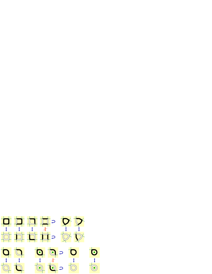
Figure 6: Illustration of the action of local gyration $H_{\gamma}$, on all the possible colourings of cycles with length $\ell\leq 4$. Punctured cycles have a green mark.

This involution has a number of important properties. It preserves the connectivity of open paths of a given colour, i.e., if $v_{1}$ and $v_{2}$ are the endpoints in $\gamma$ of a black (or a white) open path w.r.t. $\phi$, they are still the endpoints of a black (or a white) open path w.r.t. $H_{\gamma}\phi$. Furthermore, the two paths are homotopically equivalent, i.e. they can be deformed continuously the one into the other, throughout the region inside the cycle (and without crossing the puncture, if present). Then, if and only if $\phi$ consists of a monochromatic cycle, also $H_{\gamma}\phi$ has this property (and both $\phi$ and $H_{\gamma}\phi$ consist of cycles than encircle the puncture, if present). Finally, the degree of a given colour at each vertex is complemented, i.e. $\deg_{b}(v,\phi)=2-\deg_{b}(v,H_{\gamma}\phi)$ and $\deg_{w}(v,\phi)=2-\deg_{w}(v,H_{\gamma}\phi)$.

This last property implies that, for FPL configurations $\phi$ on a domain $\Lambda$, if $H_{\gamma}$ is performed on a cycle $\gamma\subseteq\Lambda$, the degree constraints at the internal vertices are not necessarily preserved. However, suppose that the domain $\Lambda$ has no external vertices, i.e. all of its vertices have degree $2$ or $4$. Assume that $\Lambda$ admits a cycle decomposition $\Gamma=(\gamma_{1},\dots,\gamma_{m})$, i.e. a partition of the edge-set into graphs $\gamma_{i}$ isomorphic to cycle graphs with lengths $|\gamma_{i}|\leq 4$. Then, because of the complementation property, the involution $H_{\Gamma}=\prod_{i}H_{\gamma_{i}}$ preserves the degree constraints at all the vertices, i.e. sends FPL into FPL (note that the product is unambiguous because $H_{\gamma}$ and $H_{\gamma^{\prime}}$ commute if $\gamma$ and $\gamma^{\prime}$ are edge-disjoint cycles).

These observations imply the following

Lemma 3.1.

Let $\Lambda$ be a domain with no external vertices, and $2n$ internal vertices of degree 2. Let $\Gamma=(\gamma_{1},\dots,\gamma_{m})$ be a cycle decomposition of $\Lambda$, and let $\phi\in\mathpzc{Fpl}\!(\Lambda)$ and $\phi^{\prime}=H_{\Gamma}(\phi)$. The following properties hold:

• If two degree-2 vertices $v_{1}$, $v_{2}$ are endpoints of a black path of $\phi$, then they are endpoints of a black path of $\phi^{\prime}$. The same holds for white paths. Thus, if $\phi$ has $(\pi_{b},\pi_{w})$ black and white pairings of the endpoints, $\phi^{\prime}$ has the same black and white pairings $(\pi_{b},\pi_{w})$. Furthermore, if $\phi$ has $\ell=\ell_{b}+\ell_{w}$ cycles, also $\phi^{\prime}$ has $\ell$ cycles.

• For each $e\in\gamma_{i}$, unpunctured and with $|\gamma_{i}|\leq 3$, if $\phi(e)=b$ then $\phi^{\prime}(e)=w$, and vice versa.

• If $\Lambda$ has a planar embedding which is outer-planar w.r.t. all the degree-2 vertices, then $\pi_{b}$, $\pi_{w}$ are both link patterns in $\mathpzc{LP}(2n)$ (i.e., the pairings of a given colour are non-crossing w.r.t. the outer-planar embedding). The link patterns $\pi_{b}$, $\pi_{w}$ are preserved by $H_{\Gamma}$ also as punctured link patterns, in $\mathpzc{LP}^{*}(2n)$, if the puncture is outside the cycles of $\Gamma$, or it is inside a face $\gamma_{i}\in\Gamma$ with $|\gamma_{i}|=1$ or $2$. If $\ell^{*}=\ell_{b}^{*}+\ell_{w}^{*}$ is the number of cycles encircling such a puncture, this number is also preserved by $H_{\Gamma}$.

• If $\Lambda$ has a planar embedding which is outer-planar w.r.t. all the degree-2 vertices except one, then $\pi_{b}$, $\pi_{w}$ are link patterns in $\mathpzc{LP}^{*}(2n-1)$, with the puncture being the only degree-2 vertex not on the boundary, and are preserved by $H_{\Gamma}$ also as punctured link patterns. In such a case, $\ell^{*}=0$ both in $\phi$ and in $\phi^{\prime}$.

Proof.

The proof consists just in translating all the established local properties of gyrations $H_{\gamma}$ at the global level of monochromatic cycles and open paths of $\Lambda$, observing that a cycle on $\Lambda$ is either one of the $\gamma_{i}\in\Gamma$, or is the concatenation of two or more open paths contained in the $\gamma_{i}$’s, and that an open path is the concatenation of one or more open paths contained in the $\gamma_{i}$’s. ∎

The class of graphs $\Lambda$ allowing for a cycle decomposition, and thus a gyration operation $H_{\Gamma}$ with the properties above, is very large. Furthermore, for outer-planar graphs, in principle multiple punctures can be introduced simultaneously (e.g., at several inequivalent points which are all outside the cycles $\gamma_{i}$). However, in such a case the properties deduced from Lemma 3.1 are not specially useful.

On the contrary, if we require the presence of two inequivalent operations, the deduced properties become much more interesting, but the class of domains becomes much more narrow, and no more than one puncture can be introduced. The dihedral domains described in the previous section have the characteristics above.

If $\Lambda$ is a graph with all vertices of degree 1, 2 or 4, equipped with a planar embedding, outer-planar w.r.t. the vertices of degree 1, we have two associated graphs $\Lambda_{\pm}$ with no external vertices, for the two possible pairing of consecutive external vertices (see Figure 7 for an example). A FPL $\phi$ on $\Lambda$ induces also FPL’s both on $\Lambda_{+}$ and $\Lambda_{-}$ if and only if we have alternating boundary conditions on $\Lambda$.

Consider the case in which $\Lambda$ is a dihedral domain with $2N$ external vertices. As explained in Section 3.2, we have a reference corner, a reference side, associated to an external line, and a natural counter-clockwise labeling of the external edges.

The graphs $\Lambda_{\pm}$ inherit the planar embedding from $\Lambda$. Moreover, through the induced structure of two-dimensional cell complex, they have obvious cycle decompositions $\Gamma_{\pm}$. The two gyration operations, $H_{\Gamma_{+}}$ on $\Lambda_{+}$ and $H_{\Gamma_{-}}$ on $\Lambda_{-}$, will be just called $H_{+}$ and $H_{-}$ in the following.

Figure 7: Left: a typical domain $\Lambda$. If the reference corner is at the bottom left, the reference side is the bottom row, and the FPL configuration shown is in $\mathpzc{Fpl}\!_{+}(\Lambda)$. Middle and right: the construction of $\Lambda_{+}$ and $\Lambda_{-}$, respectively.

All the external edges $e$ of $\Lambda$ are in $\Lambda_{\pm}$ within cycles $\gamma_{i}$ of length at most 3, so that the property b of Lemma 3.1 applies. This is important in order to establish that the operations $H_{\pm}$, which act on $\Lambda_{\pm}$, when reinterpreted at the level of $\Lambda$ induce two involutions on $\mathpzc{Fpl}\!(\Lambda)$, which are bijections between $\mathpzc{Fpl}\!_{+}(\Lambda)$ and $\mathpzc{Fpl}\!_{-}(\Lambda)$. Another important aspect is that the property of preserving $\pi_{b}$, $\pi_{w}$, $\ell$ and (if applicable) $\ell^{*}$ on $\Lambda_{\pm}$ has a counterpart also on $\Lambda$.

In order to see this, at the level of generality required for the refined Razumov–Stroganov correspondence, we introduce a general class of maps that associate a link pattern to a FPL configuration. For $v$ an external vertex of $\Lambda$ such that the adjacent edge has boundary condition black, we let $\Pi(\phi,v)$ the map that associates to $\phi$ the black link pattern, with label $1$ associated to vertex $v$, and so on up to $N$ with increasing labels in counter-clockwise order. Two special cases of $\Pi(\phi,v)$ are mostly used in the following. For $\phi\in\mathpzc{Fpl}\!_{+}(\Lambda)$, we define $\Pi_{+}(\phi)=\Pi(\phi,1)$, i.e. the external vertex with label $1$ is the first one of the reference side, next to the reference corner. This is the ‘ordinary’ map used in the correspondence, i.e. $\Pi_{+}(\phi)=\pi(\phi)$ in the notations of the introduction. Then, for $\phi\in\mathpzc{Fpl}\!_{b}(\Lambda)$, we set $\Pi_{b}(\phi)=\Pi(\phi,h(\phi))$, i.e. the counting starts from the refinement position. This is the ‘new’ map introduced in this paper, i.e. $\Pi_{b}(\phi)=\tilde{\pi}(\phi)$ in the notations of the introduction (see Figure 1).

Remark that, as we have alternating boundary conditions, if the $v$-th external edge is black, the set of black external edges is $\{\ldots,v-2,v,v+2,\ldots\}$, and as a consequence

$$\Pi(\phi,v+2)=R^{-1}\Pi(\phi,v)\,.$$ (36)

Both maps $H_{\pm}$ are involutions. They do not commute among themselves, and clearly $(H_{+}H_{-})^{-1}=H_{-}H_{+}$, so the only irreducible elements in the generated monoid are strings of the form $\cdots H_{-}H_{+}H_{-}H_{+}\cdots$. It is thus convenient to call $H:\mathpzc{Fpl}\!(\Lambda)\rightarrow\mathpzc{Fpl}\!(\Lambda)$ the map

$$H(\phi)=\left\{\begin{array}[]{ll}H_{+}(\phi)&\textrm{if $\phi\in\mathpzc{Fpl}\!_{+}(\Lambda)$;}\\ H_{-}(\phi)&\textrm{if $\phi\in\mathpzc{Fpl}\!_{-}(\Lambda)$.}\end{array}\right.$$ (37)

Acting on $\mathpzc{Fpl}\!_{+}(\Lambda)$ we have

$$H^{k}(\phi) =\underbrace{H_{(-1)^{k-1}}\cdots H_{-}H_{+}}_{k}(\phi)\,; H^{-k}(\phi) =\underbrace{H_{(-1)^{k}}\cdots H_{+}H_{-}}_{k}(\phi)\,;$$ (38)

and the irreducible elements of the monoid are just the powers $\{H^{k}\}_{k\in\mathbb{Z}}$.

The following lemma, due to Wieland in the case of the square [14], is deduced easily from Lemma 3.1 and the construction of $\Lambda_{\pm}$ from a domain $\Lambda$ described above, and will be at basis of the reasonings in Section 4

Lemma 3.2 (Wieland half-gyration lemma).

Let $\Lambda$ be a dihedral domain, $\phi\in\mathpzc{Fpl}\!(\Lambda)$ and $v$ an external vertex of $\Lambda$ adjacent to a black edge of $\phi$. Then

$$\Pi(H(\phi),v+1)=\Pi(\phi,v)\,,$$ (39)

and in particular

$$\Pi(H^{2}(\phi),v)=R\,\Pi(\phi,v)\,.$$ (40)

Proof.

Say that $v$ is odd, so that $\phi\in\mathpzc{Fpl}\!_{+}(\Lambda)$ and $H\equiv H_{+}$. In $\Lambda_{+}$, the vertex $v$ is paired to $v+1$. After the application of $H$, the link pattern $\pi_{b}$ is preserved on $\Lambda_{+}$. We can split back the vertices, to obtain a configuration in $\mathpzc{Fpl}\!_{-}(\Lambda)$. In particular, as we can apply the property b of Lemma 3.1 to the edges adjacent to $v$ and $v+1$, in $H(\phi)$ the black edge is now adjacent to $v+1$, from which equation (39) follows. If $v$ is even, the reasoning is analogous. In particular, because of the staggered choice of equation (37), it is still true that $v$ is paired to $v+1$. Equation (40) comes from applying (39) twice and then (36): $\Pi(\phi,v)=\Pi(H^{2}(\phi),v+2)=R^{-1}\Pi(H^{2}(\phi),v)$. ∎

A stronger version of the lemma (that we do not use in this paper), still due to Wieland in the case of the square, considers the triple $(\pi_{b},\pi_{w},\ell)$, or, in case of $\mathpzc{LP}(\Lambda)=\mathpzc{LP}^{*}(2n)$, the quadruple $(\pi_{b},\pi_{w},\ell,\ell^{*})$. Let ${\bm{\Pi}}(\phi,v,v^{\prime})=\xi^{\ell(\phi)}\eta^{\ell^{*}(\phi)}\;\Pi(\phi,v)\otimes\Pi(\sigma\phi,v^{\prime})$ (with $\ell^{*}(\phi)\equiv 0$ if not applicable). Then we have

Lemma 3.3.

Let $\Lambda$ be a dihedral domain, $\phi\in\mathpzc{Fpl}\!(\Lambda)$ and $v$, $v^{\prime}$ external vertices of $\Lambda$ adjacent to a black and a white edge of $\phi$, respectively. Then

$${\bm{\Pi}}(H(\phi),v+1,v^{\prime}-1)={\bm{\Pi}}(\phi,v,v^{\prime})\,,$$ (41)

and in particular

$${\bm{\Pi}}(H^{2}(\phi),v,v^{\prime})=(R\otimes R^{-1})\circ{\bm{\Pi}}(\phi,v,v^{\prime})\,.$$ (42)

The Wieland gyration theorem of [14], generalised to dihedral domains, then follows as a corollary of equations (40) and (42).

Theorem 3.1 (Wieland gyration theorem).

Let $\Lambda$ be a dihedral domain, and $\Psi_{\Lambda}(\pi)$ the number of FPL $\phi\in\mathpzc{Fpl}\!_{+}(\Lambda)$ such that $\Pi_{+}(\phi)=\pi$. Then

$$\Psi_{\Lambda}(\pi)=\Psi_{\Lambda}(R^{-1}\pi)\,.$$ (43)

Similarly, for $\Psi_{\Lambda}(\pi_{b},\pi_{w},\ell,\ell^{*})$ the number of FPL $\phi\in\mathpzc{Fpl}\!_{+}(\Lambda)$ with the corresponding quadruple $(\pi_{b},\pi_{w},\ell,\ell^{*})$, with $\pi_{b}=\Pi(\phi,1)=\Pi_{+}(\phi)$, $\pi_{w}=\Pi(\sigma\phi,2)=\Pi_{+}(H_{-}\sigma\phi)$, and $\ell^{*}(\phi)$ if applicable,

$$\Psi_{\Lambda}(\pi_{b},\pi_{w},\ell,\ell^{*})=\Psi_{\Lambda}(\pi_{w},\pi_{b},\ell,\ell^{*})=\Psi_{\Lambda}(R^{-1}\pi_{b},R\pi_{w},\ell,\ell^{*})\,.$$ (44)

4 The Razumov–Stroganov correspondence for the Scattering Matrix

This section is mainly devoted to the proof of Theorem 4.1, that relates the solution of the scattering equation, on the $O(1)$ Dense Loop Model side, to the enumeration of FPL’s performed according to the refinement position, and the link pattern evaluated with the map $\Pi_{b}$.

4.1 The correspondence for the enumerations according to $\Pi_{b}$

In the previous sections we gathered all the ingredients required for stating and proving our main result. Assume that a dihedral domain $\Lambda$ is given, and fix a reference side $r$ on the boundary, of length $L$. Call $h(\phi)\in\{1,\ldots,L\}$ the function associating to a FPL configuration $\phi$ its refinement position along $r$, counted in counter-clockwise order (starting from the reference corner). Define the vector $|\Psi_{\Lambda}(t)\rangle$ whose components $\Psi_{\Lambda}(t;\pi)$ are enumerations of FPL in $\mathpzc{Fpl}\!_{b}(\Lambda)$, with link pattern associated through the function $\Pi_{b}$, and weighted according to the refinement position, i.e.

$$\mbox{$|\Psi_{\Lambda}(t)\rangle$}:=\sum_{\pi\in\mathpzc{LP}(\Lambda)}\Psi_{\Lambda}(t;\pi)\mbox{$|\pi\rangle$}=\sum_{\phi\in\mathpzc{Fpl}\!_{b}(\Lambda)}t^{h(\phi)-1}\mbox{$|\Pi_{b}(\phi)\rangle$}\,.$$ (45)

This section is devoted to the proof of the following

Theorem 4.1.

The vector $|\Psi_{\Lambda}(t)\rangle$ defined above satisfies the scattering equation at $i=1$, equation (9), i.e.

$$X_{1}(t)\mbox{$|\Psi_{\Lambda}(t)\rangle$}=R\,\mbox{$|\Psi_{\Lambda}(t)\rangle$}\,.$$ (46)

In other words, for all choices of dihedral domain $\Lambda$, and reference side $r$ of $\Lambda$,

$$\mbox{$|\Psi_{\Lambda}(t)\rangle$}=K_{\Lambda}(t)\;\mbox{$|\Psi^{(1)}_{O(1)}(t)\rangle$}\,,$$ (47)

where $K_{\Lambda}(t)$ is a polynomial with positive integer coefficients, depending on $\Lambda$ and $r$, and $|\Psi^{(1)}_{O(1)}(t)\rangle$ is the solution for the representation on the space $\mathpzc{LP}(\Lambda)$.

An illustration of this theorem is given in Figure 8.

Figure 8: Top: the 7 FPL on the $3\times 3$ square, collected according to the enumeration $\Pi_{b}$. Middle: analogous enumeration of the 14 FPL on the domain $\Lambda=(4,4;0,0,0,2)$. The enumerations are proportional, by a factor $1+t$. Bottom rows: the three summands involved in the scattering equation. These rows sum up to zero, so the scattering equation is satisfied by the enumeration vectors.

For $\ast=+,-,b,w$, call $\mathpzc{Fpl}\!_{\ast}^{[i]}(\Lambda)$ the restriction of $\mathpzc{Fpl}\!_{\ast}(\Lambda)$ to configurations such that $h(\phi)=i$. Call $|\Psi_{\Lambda}^{[i]}\rangle$ the vector whose components are enumerations of $\mathpzc{Fpl}\!_{b}^{[i]}(\Lambda)$, using $\Pi_{b}$. We can write $|\Psi_{\Lambda}(t)\rangle$ as

$$\mbox{$|\Psi_{\Lambda}(t)\rangle$}=\sum_{i=1}^{L}t^{i-1}\mbox{$|\Psi_{\Lambda}^{[i]}\rangle$}=\sum_{\pi\in\mathpzc{LP}(\Lambda)}t^{i-1}\Psi_{\Lambda}^{[i]}(\pi)\mbox{$|\pi\rangle$}=\sum_{i=1}^{L}t^{i-1}\!\!\!\sum_{\phi\in\mathpzc{Fpl}\!_{b}^{[i]}(\Lambda)}\!\!\!\mbox{$|\Pi_{b}(\phi)\rangle$}\,.$$ (48)

As a consequence of Proposition 2.1, the proof of Theorem 4.1 splits into the two lemmas

Lemma 4.1.

The vectors $|\Psi_{\Lambda}^{[i]}\rangle$ satisfy

$$({\bf e}_{1}-R\,{\bf e}_{N})\mbox{$|\Psi_{\Lambda}^{[i]}\rangle$}=0\,;$$ (49)

Lemma 4.2.

For any $\pi\in\mathpzc{LP}(\Lambda)$ such that $1\includegraphics{fig_nsim.eps}2$ we have

$$t\Psi_{\Lambda}(t;\pi)=\Psi_{\Lambda}(t,R^{-1}\pi)\,.$$ (50)

We prove these lemmas in the remainder of this subsection. Before this, we need some notations. In Section 2 we introduced a space $\mathbb{C}^{\mathpzc{LP}(\Lambda)}$, in order to conveniently encode the action of Temperley–Lieb Algebra through linear operators. Later on, we have introduced maps $\Pi(\phi,v)$ from the set $\mathpzc{Fpl}\!(\Lambda)$ (or variants) to $\mathpzc{LP}(\Lambda)$. Here we will also consider the spaces $\mathbb{C}^{\mathpzc{Fpl}\!_{\ast}(\Lambda)}$, with $\ast=+,-,b,w$, for which a canonical basis is given by the configurations, $\|\phi\rangle\!\rangle$, in order to promote also the maps $\Pi(\phi,v)$ to linear operators. Note that, for easiness of notation, we use a different graphical representation for vectors in $\mathbb{C}^{\mathpzc{LP}(\Lambda)}$, such as $|\pi\rangle$, and vectors in $\mathbb{C}^{\mathpzc{Fpl}\!(\Lambda)}$, such as $\|\phi\rangle\!\rangle$.

With abuse of notation, we will still call $\Pi_{+}$ and $\Pi_{b}$ the linear operators associated to the maps $\Pi_{+}:\mathpzc{Fpl}\!_{+}(\Lambda)\rightarrow\mathpzc{LP}(\Lambda)$ and $\Pi_{b}:\mathpzc{Fpl}\!_{b}(\Lambda)\rightarrow\mathpzc{LP}(\Lambda)$, whose action on basis elements is $\Pi_{+}\mbox{$\|\phi\rangle\!\rangle$}=\mbox{$|\Pi_{+}(\phi)\rangle$}$ and $\Pi_{b}\mbox{$\|\phi\rangle\!\rangle$}=\mbox{$|\Pi_{b}(\phi)\rangle$}$. Define the vector associated to the collection of configurations in $\mathpzc{Fpl}\!_{b}(\Lambda)$, weighted with their refinement position, as

$$\mbox{$\|s_{\Lambda}(t)\rangle\!\rangle$}:=\sum_{\phi\in\mathpzc{Fpl}\!_{b}(\Lambda)}t^{h(\phi)-1}\mbox{$\|\phi\rangle\!\rangle$}\,.$$ (51)

The vector $|\Psi_{\Lambda}(t)\rangle$ is thus the image of $\|s_{\Lambda}(t)\rangle\!\rangle$ under the map $\Pi_{b}$, $\mbox{$|\Psi_{\Lambda}(t)\rangle$}=\Pi_{b}\mbox{$\|s_{\Lambda}(t)\rangle\!\rangle$}$. Similarly, calling

$$\mbox{$\|s_{\Lambda}^{[i]}\rangle\!\rangle$}:=\sum_{\phi\in\mathpzc{Fpl}\!_{b}^{[i]}(\Lambda)}\mbox{$\|\phi\rangle\!\rangle$}\,,$$ (52)

we have $\mbox{$|\Psi_{\Lambda}^{[i]}\rangle$}=\Pi_{b}\mbox{$\|s_{\Lambda}^{[i]}\rangle\!\rangle$}$.

Proof of Lemma 4.1:  This lemma was already proven in [3] (Proposition 4.4, equation (61)), when the domain $\Lambda$ was a $n\times n$ square. Actually, the proof easily extends to the general class of domains $\Lambda$ that we described in Section 3.2, which is also the generality of the treatment of Wieland gyration discussed in Section 3 of [3].

We want to give here a slightly reformulated proof. First, we define two involutions $\tilde{\bf e}_{1}$ and $\tilde{\bf e}_{N}$ on $\mathpzc{Fpl}\!(\Lambda)$. These operators are conjugated versions of the local gyration $H_{\gamma}$, for $\gamma_{1}$ and $\gamma_{N}$ certain cycles in the graph, adjacent to the refinement position. If $\phi\in\mathpzc{Fpl}\!_{+}$, $\gamma_{1}$ and $\gamma_{N}$ are the faces at the top-right and top-left corner of the refinement $h(\phi)$, respectively. If $\phi\in\mathpzc{Fpl}\!_{-}$, right and left are interchanged.

The operator $\tilde{\bf e}_{1}$ flips the cycle $\gamma_{1}$, if it has length 4 and it is coloured in an alternating way, i.e. of the form       or      , otherwise it leaves the FPL unchanged. The operator $\tilde{\bf e}_{N}$ has an analogous action on $\gamma_{N}$. The local configurations which are not kept fixed are

If $\phi\in\mathpzc{Fpl}\!_{b}(\Lambda)$, the operators $\tilde{\bf e}_{1}$ and $\tilde{\bf e}_{N}$ act analogously to the Temperley–Lieb generators ${\bf e}_{1}$ and ${\bf e}_{N}$, in the sense that it holds

$$\Pi(\tilde{\bf e}_{N}\phi,h(\phi)) ={\bf e}_{N}\Pi(\phi,h(\phi))={\bf e}_{N}\Pi_{b}(\phi)\,;$$ (53a)

$$\Pi(\tilde{\bf e}_{1}\phi,h(\phi)) ={\bf e}_{1}\Pi(\phi,h(\phi))={\bf e}_{1}\Pi_{b}(\phi)\,.$$ (53b)

Consider the state $\|s_{\Lambda}^{[i]}\rangle\!\rangle$ (so $i=h(\phi)$ for all contributing configurations). We claim that

$$H\,\tilde{\bf e}_{N}\mbox{$\|s_{\Lambda}^{[i]}\rangle\!\rangle$}=\sigma\mbox{$\|s_{\Lambda}^{[i]}\rangle\!\rangle$}=H^{-1}\tilde{\bf e}_{1}\mbox{$\|s_{\Lambda}^{[i]}\rangle\!\rangle$}\,.$$ (54)

In other words, the three maps $\sigma$, $H\,\tilde{\bf e}_{N}$ and $H^{-1}\tilde{\bf e}_{1}$ are bijections from $\mathpzc{Fpl}\!_{b}^{[i]}(\Lambda)$ to $\mathpzc{Fpl}\!_{w}^{[i]}(\Lambda)$ (this is clear for $\sigma$). It is obvious, from the fact that $\sigma$, $H$, $\tilde{\bf e}_{1}$ and $\tilde{\bf e}_{N}$ are all invertible, that they are bijections on $\mathpzc{Fpl}\!(\Lambda)$, and the only fact that needs to be checked is that, in both non-trivial cases, the image of a FPL with refinement position $i$, and black, is a FPL with refinement position $i$, and white. Figure 9 shows this fact for $H\,\tilde{\bf e}_{N}$.

Figure 9: Analysis of the map $H\tilde{\bf e}_{N}$ on $\mathpzc{Fpl}\!_{b}^{[i]}(\Lambda)$. The state $\|s_{\Lambda}^{[i]}\rangle\!\rangle$ is decomposed according to the colour of the edge marked with ‘?’. The action of $\tilde{\bf e}_{N}$ is non-trivial if and only if this edge is white. Then, we can analyse the action of $H$, by producing the graph $\Lambda_{+}$. The result is the decomposition, according to the colour of the edge marked with ‘?’, of the state $\sigma\mbox{$\|s_{\Lambda}^{[i]}\rangle\!\rangle$}$.

Equations (53) allow to deduce

$$\begin{split}{\bf e}_{N}\mbox{$|\Psi_{\Lambda}^{[i]}\rangle$}&={\bf e}_{N}\Pi_{b}\mbox{$\|s_{\Lambda}^{[i]}\rangle\!\rangle$}=\Pi(\cdot,i)\,\tilde{\bf e}_{N}(i)\,\mbox{$\|s_{\Lambda}^{[i]}\rangle\!\rangle$}\,.\end{split}$$ (55a)

$$\begin{split}{\bf e}_{1}\mbox{$|\Psi_{\Lambda}^{[i]}\rangle$}&={\bf e}_{1}\Pi_{b}\mbox{$\|s_{\Lambda}^{[i]}\rangle\!\rangle$}=\Pi(\cdot,i)\,\tilde{\bf e}_{1}(i)\,\mbox{$\|s_{\Lambda}^{[i]}\rangle\!\rangle$}\,.\end{split}$$ (55b)

We can now compare the two left hand sides of (55), using (54) and (40)

$$\begin{split}{\bf e}_{1}\mbox{$|\Psi_{\Lambda}^{[i]}\rangle$}&=\Pi(\cdot,i)\,H^{2}\tilde{\bf e}_{N}(i)\,\mbox{$\|s_{\Lambda}^{[i]}\rangle\!\rangle$}=R\,\Pi(\cdot,i)\,\tilde{\bf e}_{N}(i)\,\mbox{$\|s_{\Lambda}^{[i]}\rangle\!\rangle$}=R\,{\bf e}_{N}\mbox{$|\Psi_{\Lambda}^{[i]}\rangle$}\,;\end{split}$$ (56)

as was to be proven. ∎

Proof of Lemma 4.2:  Consider a pattern $\pi\in\mathpzc{LP}(\Lambda)$ such that $1\includegraphics{fig_nsim.eps}2$. We claim that, for every $\phi\in\mathpzc{Fpl}\!_{b}(\Lambda)$ such that $\Pi_{b}(\phi)=\pi$ and $h(\phi)=h$, the configuration $\phi^{\prime}=H^{-1}(\phi)$ has $\Pi_{b}(\phi^{\prime})=R^{-1}\pi$ and $h(\phi^{\prime})=h+1$. In particular it has $N\includegraphics{fig_nsim.eps}1$. This is easily seen from the local properties of gyration, in a neighbourhood of the refinement position (see Figure 10, right to left). Analogously, for a pattern $\pi\in\mathpzc{LP}(\Lambda)$ such that $N\includegraphics{fig_nsim.eps}1$, for every $\phi\in\mathpzc{Fpl}\!_{b}(\Lambda)$ such that $\Pi_{b}(\phi)=\pi$ and $h(\phi)=h$, the configuration $\phi^{\prime}=H(\phi)$ has $\Pi_{b}(\phi^{\prime})=R\,\pi$ and $h(\phi^{\prime})=h-1$ (see Figure 10, left to right).

Figure 10: Analysis of Wieland half-gyration in a neighbourhood of the refinement position, required in the proof of Lemma 4.2.

Thus, $H$ induces a bijection between the sets of configurations in $\mathpzc{Fpl}\!_{b}(\Lambda)$ with link pattern $\pi$ and $R^{-1}\pi$, given that $1\includegraphics{fig_nsim.eps}2$ in $\pi$ and thus $N\includegraphics{fig_nsim.eps}1$ in $R^{-1}\pi$. As this bijection acts in a simple way on the refinement position, it induces a relation at the level of the weighted generating functions, $\Psi_{\Lambda}(t;\pi)$ and $\Psi_{\Lambda}(t;R^{-1}\pi)$, which is exactly the statement of the lemma. ∎

4.2 Special families of dihedral domains

In the definition of the vector $|\Psi_{\Lambda}(t)\rangle$ there is an implicit dependence from the reference side. A generic dihedral domain has several (at most $4$) possible choices of reference side $r$, which, except for the case of the $n\times n$ square and a few other symmetric cases, are in general not equivalent.

In this section we analyse this aspect, so, only within this section, we adopt a notation that makes explicit the dependence on the reference side $r$, by writing $|\Psi_{{\Lambda,r}}(t)\rangle$ for the vector, and $K_{{\Lambda,r}}(t)$ for the proportionality factor with the minimal solution of the scattering equation, i.e.

$$\mbox{$|\Psi_{{\Lambda,r}}(t)\rangle$}=K_{{\Lambda,r}}(t)\,\mbox{$|\Psi_{O(1)}^{(1)}(t)\rangle$}\,.$$ (57)

Interestingly, for all the three possible realisations on the correspondence, $\mathpzc{LP}(\Lambda)=\mathpzc{LP}(2n)$, $\mathpzc{LP}^{*}(2n)$ or $\mathpzc{LP}^{*}(2n-1)$, there exists a dihedral domain (and a reference side) realising the minimal degree, i.e. such that $K_{{\Lambda,r}}(t)$ is a constant, and in fact can be set to $1$.

For $\mathpzc{LP}(\Lambda)=\mathpzc{LP}(2n)$, the realisation with minimal degree corresponds to the $n\times n$ square domain, while for $\mathpzc{LP}(\Lambda)=\mathpzc{LP}^{*}(N)$ (either even or odd) the realisation with minimal degree corresponds to Half-turn symmetric ASM of size $N$ (refer back to Figure 5). Indeed, ordinary ASM’s on the square of side $n$ have refinement positions in the range $\{1,\ldots,n\}$, thus the corresponding polynomials $\Psi_{\Lambda}(t;\pi)$ have degree at most $n-1$. Similarly, HTASM’s of side $N$ have refinement positions in the range $\{1,\ldots,N\}$, thus the corresponding polynomials $\Psi_{\Lambda}(t;\pi)$ have degree at most $N-1$. As observed at the end of Section 3.2, both ASM and HTASM are special cases of dihedral domains, and the latter allows for the presence of a puncture. Furthermore, it is easily seen that for each rainbow pattern in $\mathpzc{LP}(2n)$ there exists a unique ASM of size $n$, and that for each rainbow pattern in $\mathpzc{LP}^{*}(N)$ there exists a unique HTASM of size $N$.

As we have proven that ASM’s on the square present refined dihedral Razumov–Stroganov correspondence on the link-pattern space $\mathpzc{LP}(2n)$, and that HTASM’s present refined dihedral Razumov–Stroganov correspondence on the link-pattern space $\mathpzc{LP}^{*}(N)$, the reasonings of the previous paragraph imply upper bounds on the degree of $\Psi_{O(1)}^{(1)}(t)$, in the two cases $\mathpzc{LP}(2n)$ and $\mathpzc{LP}^{*}(N)$. As these bounds match the lower bounds in Corollary 2.1, we get the following

Proposition 4.1.

For $\mathpzc{LP}(2n)$, there exist polynomial solutions $|\Psi^{(i)}(t)\rangle$ of the scattering equation (9), such that the components $\Psi^{(i)}(t;\pi)$ are polynomials in $t$ with positive integer coefficients, the maximal (over $\pi$’s) degree is $n-1$, and $\Psi^{(i)}(t;\pi)=t^{j}$ for some $j$ if $\pi$ is a rainbow pattern. For $\mathpzc{LP}^{*}(N)$, the same facts do hold, with maximal degree $N-1$.

For a generic dihedral domain $\Lambda$, the space $\mathpzc{LP}(\Lambda)$ is independent from the reference side $r$, and thus also the DLM vector $|\Psi_{O(1)}^{(1)}(t)\rangle$ is the same. However, since the external lines are possibly of different lengths, and the range of allowed possible refinement positions, i.e. indices $h$ such that $\mbox{$|\Psi_{{\Lambda,r}}^{[h]}\rangle$}\neq 0$, may be different for different sides $r$, the vectors $|\Psi_{{\Lambda,r}}(t)\rangle$, for a given $\Lambda$ and the various possible choices of $r$, are in general distinct polynomials, and even of different degree. Our result implies that this difference arises uniquely at the level of the overall factor $K_{{\Lambda,r}}(t)$.

A sub-family of dihedral domains in which this feature can be seen explicitly is the one with three corners (this is the maximum allowed number, besides the ‘classical’ $n\times n$ square). We can set $a_{1}=a_{2}=a_{3}=0$, and $a_{4}>0$, without loss of generality. These domains also minimize the number of ‘crossing bundles’ (again, besides the case of the square): we have three bundles crossing each other, of width $a_{4}$, $L_{x}-a_{4}$ and $L_{y}-a_{4}$.

A useful and more symmetric parametrisation consists in setting $L_{x}=\alpha+2\beta+\gamma$, $L_{y}=\alpha+\beta+2\gamma$ and $a_{4}=\beta+\gamma$, so that the bundles have widths $\alpha+\beta$, $\alpha+\gamma$ and $\beta+\gamma$. We call such a domain a three-bundle domain, or triangoloid, $T(\alpha,\beta,\gamma)$ (see Figure 11). There are three possible choices of reference sides, $r(\alpha)$, $r(\beta)$ and $r(\gamma)$, of lengths $2\alpha+\beta+\gamma$, $\alpha+2\beta+\gamma$ and $\alpha+\beta+2\gamma$, respectively. The number of external edges of each colour is $2n=2(\alpha+\beta+\gamma)$ (we use $n$ as a synonim of $\alpha+\beta+\gamma$ in what follows). Since $T(\alpha,\beta,\gamma)$ has no faces with less than three edges, the correspondence holds with the non-punctured link patterns, $\mathpzc{LP}(\Lambda)=\mathpzc{LP}(2n)$.

Figure 11: A three-bundle domain $T(\alpha,\beta,\gamma)$, with $(\alpha,\beta,\gamma)=(2,3,4)$. The reference side has length $\alpha+2\gamma+\beta=13$.

We thus have $\mbox{$|\Psi_{T(\alpha,\beta,\gamma),r(\gamma)}(t)\rangle$}=K_{T(\alpha,\beta,\gamma),r(\gamma)}(t)\;\mbox{$|\Psi_{\mathpzc{LP}(2n)}(t)\rangle$}$, or, with a more compact ad hoc notation,

$$\mbox{$|\Psi_{\alpha,\beta|\gamma}(t)\rangle$}=K_{\alpha,\beta|\gamma}(t)\;\mbox{$|\Psi_{\mathpzc{LP}(2n)}(t)\rangle$}\,.$$ (58)

Simple reasonings (of reflection symmetry) show that $K_{\alpha,\beta|\gamma}(t)$ is symmetric under interchange of $\alpha$ and $\beta$, and $t\to 1/t$ (up to an appropriate rescaling by $t^{\gamma}$, because $\gamma=L-n$). Here we report a formula for $K_{\alpha,\beta|\gamma}(t)$, without providing a proof 

$$\begin{split}K_{\alpha,\beta|\gamma}(t)&=\det_{1\leq i,j\leq\gamma}\left(\binom{\alpha+\beta-1}{\beta-i+j}+t\,\binom{\alpha+\beta-1}{\beta-i+j-1}\right)\\ &=\frac{\Delta_{\alpha}\Delta_{\beta}\Delta_{\gamma+1}\Delta_{\alpha+\beta+\gamma-1}}{\Delta_{\alpha+\beta-1}\Delta_{\alpha+\gamma}\Delta_{\beta+\gamma}}\;\sum_{i=0}^{\gamma}t^{i}\binom{\beta-1+i}{i}\binom{\alpha-1+\gamma-i}{\gamma-i}\,,\end{split}$$ (59)

where $\Delta_{n}=\prod_{k=0}^{n-1}k!$. The function $K_{\alpha,\beta|\gamma}(t)$ has also a combinatorial interpretation in terms of the weighted enumerations of rhombus tilings of a hexagon with sides $(\alpha,\beta,\gamma)$. As well as ASM’s, rhombus tilings of a hexagon have a natural notion of refinement position w.r.t. a given side (defined as the position of the only lozenge, adjacent to the side, with the longer diagonal orthogonal to the side). In our case, a tiling has a weight $t^{h-1}$, for $h$ the refinement position w.r.t. one of the two sides of length $\gamma$ (see Figure 12).

This connection between lozenge tilings of a hexagon and the factor $K_{\Lambda,r}$ for the Razumov–Stroganov correspondence on three-bundle domains has also a direct combinatorial interpretation through an analysis of frozen regions in configurations with rainbow link patterns.

   

Figure 12: Left: example of weighted rhombus tiling corresponding to the expression in (59). Right: the associated dimer covering of a region of the honeycomb lattice.

4.3 Specialisations to $t=1$ and $t=0$

As explained in Section 2.2, there are two relavant specialisations of the parameter $t$. When $t=1$, the vector $|\Psi_{\Lambda}(1)\rangle$ is the ground state of the Hamiltonian of the $O(1)$ Dense Loop Model, equation (6). This means that we have a realisation of the Razumov–Stroganov correspondence involving a different class of FPL’s on a domain $\Lambda$, namely $\mathpzc{Fpl}\!_{b}(\Lambda)$ and a different function associating a link pattern, namely $\Pi_{b}(\phi)$. One way to obtain from this result the usual Razumov–Stroganov correspondence, involving $\mathpzc{Fpl}\!_{+}(\Lambda)$ and $\Pi_{+}(\phi)$, will be presented in Section 5.3.

Another way to recover the usual correspondence is by looking at the specialisations $t\to 0$ (or at the symmetric limit $t\to\infty$). In Section 2.2 we have recalled a result of Di Francesco and Zinn-Justin [6], which implies that the specialisation $t=0$ of a solution of the scattering equation (9), at $i=1$, is equal to the image of the ground state of the Hamiltonian (6) of size $N-2$, under the map that inserts a short arc $(N,1)$ (see equation (32)). A correspondence is found if we can show that the analogous feature arises also on the FPL side.

Consider a domain $\Lambda=(L_{x},L_{y};0,a_{2},a_{3},a_{4})$, such that all the parameters $a_{2}$, $a_{3}$ and $a_{4}$ are at least 2 (in particular, $\Lambda$ has a single corner). In such a domain it is easily seen that $\mbox{$|\Psi_{\Lambda}^{[1]}\rangle$}=0$, while, as we now deduce, the expression $\mbox{$|\Psi_{\Lambda}^{[2]}\rangle$}=\lim_{t\to 0}\frac{1}{t}\mbox{$|\Psi_{\Lambda}(t)\rangle$}$ can be related to the ordinary enumeration of FPL on a suitable reduced domain $\Lambda^{\prime}$.

Figure 13: Frozen region induced by imposing that the refinement position is 2, on a domain $\Lambda=(L_{x},L_{y};0,a_{2},a_{3},a_{4})$ such that all the parameters $a_{2}$, $a_{3}$ and $a_{4}$ are at least 2. The light-yellow unfrozen region is the associated reduced domain $\Lambda^{\prime}$. Left: $\Lambda^{\prime}$ corresponds to ordinary ASM’s, and has the maximal number of corners, 4. Right: $\Lambda^{\prime}$ has the minimal number of corners, 1.

More precisely, within $|\Psi_{\Lambda}^{[2]}\rangle$ the only non-vanishing components have $1\includegraphics{fig_sim.eps}N$, as this connection is implied by the tile at the refinement position and the induced frozen region (and the puncture, if any, is within the unfrozen region and thus not surrounded by this short arc). The unfrozen region corresponds to the domain $\Lambda^{\prime}=(L_{x}-4,L_{y}-4;0,a_{2}-2,a_{3}-2,a_{4}-2)$, and has induced alternating boundary conditions, with a white external edge adjacent to the reference corner. Thus the FPL’s $\phi$ in $\mathpzc{Fpl}\!_{b}^{[2]}(\Lambda)$ are in bijection with the FPL’s $\phi^{\prime}$ in $\mathpzc{Fpl}\!_{-}(\Lambda^{\prime})$. The external edges in $\Lambda^{\prime}$ are connected to the external edges in $\Lambda$, numbered from $2$ to $N-1$, in counter-clockwise order starting from the reference corner, thus, for $\phi$ and $\phi^{\prime}$ configurations in bijection, the link patterns $\Pi_{-}(\phi^{\prime})$ and $\Pi_{b}(\phi)$ are easily related. See also Figure 13. This gives

$$\Psi_{\Lambda}^{[2]}(\begin{picture}(8.0,2.8)\put(0.0,0.0){\includegraphics[scale={1.2}]{fig_LP_iim2.eps}} \put(0.6,-1.0){${}_{1}\rule{30.0pt}{0.0pt}{}_{N}$} \put(3.5,0.6){$\pi$} \end{picture})=\Psi_{\Lambda^{\prime}}(1,\pi)\,,$$ (60)

and therefore, in view of equation (32), $|\Psi_{\Lambda^{\prime}}(1)\rangle$ is the ground state of the Hamiltonian corresponding to the domain $\Lambda^{\prime}$, which means that the Razumov–Stroganov correspondence holds in the domain $\Lambda^{\prime}$.

As for every dihedral domain $\Lambda^{\prime}=(L^{\prime}_{x},L^{\prime}_{y};0,a^{\prime}_{2},a^{\prime}_{3},a^{\prime}_{4})$ we can construct a dihedral domain $\Lambda=(L^{\prime}_{x}+4,L^{\prime}_{y}+4;0,a^{\prime}_{2}+2,a^{\prime}_{3}+2,a^{\prime}_{4}+2)$ with the required properties, the reasoning above produces an alternative proof of the original Razumov–Stroganov correspondence (on all dihedral domains, and also in the punctured version).

5 From the enumerations $\Psi_{\Lambda}(t;\pi)$ to the ordinary Razumov–Stroganov correspondence and Di Francesco’s conjecture

At the end of the previous section we described a way of deriving the ordinary Razumov–Stroganov correspondence from Theorem 4.1, that makes use of a deep and general result in [6] for relating the limit $t\to 0$ of the solution of the scattering equation to the ground state of the Hamiltonian at smaller size.

Here, in Section 5.2 we provide a derivation of the more general Di Francesco’s conjecture in [5], quickly described in the introduction, and whose precise statement is reported in the following Theorem 5.1. At the light of the reasonings in Section 2.2, this also provides an alternative, self-contained proof of the ordinary Razumov–Stroganov correspondence. Then, in Section 5.3 we give a third, bijective derivation of the ordinary Razumov–Stroganov correspondence. Also this derivation does not rely on [6], and furthermore it doesn’t make use of the results of Section 5.2.

All these results follow from Theorem 4.1, and from an analysis of the structure of the orbits under the action of the half-gyration $H$, presented in Section 5.1.

5.1 Structure of the orbits under half-gyration

The orbit associated to a configuration $\phi\in\mathpzc{Fpl}\!(\Lambda)$, under the action of the half-gyration operator $H$, is defined as the sequence $(\phi,\,H\,\phi,\,H^{2}\,\phi,\,H^{3}\,\phi,\ldots,\,H^{p-1}\,\phi)$, where $p=p(\phi)$ is the smallest positive integer such that $H^{p}\phi=\phi$ (i.e., the period of the orbit).

Remark that the configurations in the list are alternating in $\mathpzc{Fpl}\!_{+}(\Lambda)$ and $\mathpzc{Fpl}\!_{-}(\Lambda)$, and in particular the period must be even. The precise periodicity of the various orbits is immaterial at our purposes, and, in order to disentangle this element from the analysis, we will mostly concentrate equivalently on the periodically-repeated infinite sequences.

Thus, for some configuration $\phi\in\mathpzc{Fpl}\!(\Lambda)$, we define ${\cal O}(\phi)$ as the infinite sequence ${\cal O}(\phi):=\{\phi_{t}\}_{t\in\mathbb{Z}}$, determined as $\phi_{0}\equiv\phi$, and $\phi_{t}=H^{t}\phi_{0}$ for $t\neq 0$, i.e.

$$\ldots\;\xrightarrow{H}\,\phi_{-2}\;\xrightarrow{H}\,\phi_{-1}\;\xrightarrow{H}\,\phi_{0}\;\xrightarrow{H}\,\phi_{1}\;\xrightarrow{H}\,\phi_{2}\;\xrightarrow{H}\,\ldots$$

(recall that $H$ is invertible). Call ${\cal O}^{p}$ a periodic portion of an infinite orbit ${\cal O}$, and ${\cal O}^{p}_{\ast}$ the part of ${\cal O}^{p}$ in $\mathpzc{Fpl}\!_{\ast}(\Lambda)$, for $\ast=+,-,b,w$.

Recall that we defined above $h(\phi)\in\{1,\ldots,L\}$ as the refinement position of $\phi$, i.e., position of the only $c$-type tile along our reference side. Define also $d(\phi)\in\{a,b,c\}$ as the direction taken at the refinement position, i.e., the kind of tile, among $\{a,b,c\}$, for the tile ‘immediately above’ the refinement position (this is well-defined for all dihedral domains, except for a few cases with size of order 1, like the $1\times 1$ square). Note that the notion of $d(\phi)$ uses the fact that the internal vertices have degree 4, but is independent from the number of sides in the neighbouring faces, and is thus well defined also for those dihedral domains in which some of the faces adjacent to the reference side are triangles. As a shortcut, for a fixed orbit ${\cal O}(\phi)$, call $h_{t}=h(\phi_{t})$ and $d_{t}=d(\phi_{t})$.

We have the following useful lemma:

Lemma 5.1.

If $\phi\in\mathpzc{Fpl}\!_{+}(\Lambda)$, the only possible local patterns for the sequence $\{(h_{t},d_{t})\}_{t\in\mathbb{Z}}$ associated to its orbit ${\cal O}(\phi)$ are

$$\begin{array}[]{r|rcccl|c|c|}\cline{2-8}\cr&\vrule\lx@intercol\hfil\textrm{local pattern}\hfil\lx@intercol\vrule\lx@intercol&\vrule\lx@intercol\hfil\textrm{condition}\hfil\lx@intercol\vrule\lx@intercol\\ \cline{7-8}\cr\rule{0.0pt}{10.5pt}&\makebox[7.0pt][l]{$\cdots$}&h_{t-1}&h_{t}&h_{t+1}&\makebox[7.0pt][r]{$\cdots$}&d_{t}&h_{t}-t\\ \cline{2-8}\cr\rule{0.0pt}{11.0pt}&\makebox[7.0pt][l]{$\cdots$}&h&h&h+1&\makebox[7.0pt][r]{$\cdots$}&a&\textrm{even}\\ \phi\in\mathpzc{Fpl}\!_{w}(\Lambda)\begin{picture}(1.0,1.0)\put(0.5,0.0){$\displaystyle{\left\{\rule{0.0pt}{16.0pt}\right.}$} \end{picture}&\makebox[7.0pt][l]{$\cdots$}&h-1&h&h+1&\makebox[7.0pt][r]{$\cdots$}&c&\textrm{even}\\ &\makebox[7.0pt][l]{$\cdots$}&h-1&h&h&\makebox[7.0pt][r]{$\cdots$}&b&\textrm{even}\\ &\makebox[7.0pt][l]{$\cdots$}&h+1&h&h&\makebox[7.0pt][r]{$\cdots$}&a&\textrm{odd}\\ \phi\in\mathpzc{Fpl}\!_{b}(\Lambda)\begin{picture}(1.0,1.0)\put(0.5,0.0){$\displaystyle{\left\{\rule{0.0pt}{16.0pt}\right.}$} \end{picture}&\makebox[7.0pt][l]{$\cdots$}&h+1&h&h-1&\makebox[7.0pt][r]{$\cdots$}&c&\textrm{odd}\\ &\makebox[7.0pt][l]{$\cdots$}&h&h&h-1&\makebox[7.0pt][r]{$\cdots$}&b&\textrm{odd}\\ \cline{2-8}\cr\end{array}\phantom{descending\rule{8.0pt}{0.0pt}}$$ (61)

If $\phi\in\mathpzc{Fpl}\!_{-}(\Lambda)$, even and odd are interchanged in the column $h_{t}-t$.

Another illustration of the table in (61) is given in Figure 14.

Figure 14: A different illustration of the statement of Lemma 5.1. We show the possible transitions, in the set of six states $(d_{t},h_{t}-t)\in\{a,b,c\}\times\{\textrm{even},\textrm{odd}\}$. The symbol in $\{-,=,+\}$ next to the arrow describes the value of $h_{t+1}-h_{t}$, in $\{-1,0,+1\}$ respectively.

Proof.

The lemma is obtained by investigation of the action of $H$, at the light of the frozen regions induced by the specialisation of $d_{t}$. Remark that the parity of $h_{t}-t$ corresponds to the fact that the half-gyration acting at time $t$ acts on the plaquette immediately at the right or at the left of the refinement position.

As the orbit involves half-gyrations, given that $\phi_{0}\in\mathpzc{Fpl}\!_{+}$, $\phi_{t}\in\mathpzc{Fpl}\!_{+}$ if $t$ is even and $\phi_{t}\in\mathpzc{Fpl}\!_{-}$ if it is odd. This implies that $\phi_{t}\in\mathpzc{Fpl}\!_{b}$ if $h_{t}-t$ is odd, and $\phi_{t}\in\mathpzc{Fpl}\!_{w}$ if it is even (at time $t=0$, the black terminations have labels $1,3,5,\ldots$). From the definition of $H$ in terms of $H_{+}$ and $H_{-}$, for both parities the black external terminations are paired to the white termination at their right, so that the black pattern rotates counter-clockwise, and the white one clockwise. This implies that we have to study the local behaviour of half-gyration only in the two situations described on the left-most column of Figure 15 (the other two choices, obtained by vertical reflection, would correspond to $H^{-1}$).

Figure 15: Illustration of the analysis of Wieland half-gyration, involved in the proof of Lemma 5.1. Graphical notations are as in the general treatment of Wieland gyration made in Section 3 of [3] (see in particular [3, Fig. 4], and Figure 7 here). More precisely, we denote in yellow only the plaquettes concerned with the operation $H$ (and not the ones concerned with $H^{-1}$), and we put a red bullet on those plaquettes that are left stable by gyration. An orange circle denotes the refinement position.

The two situations are very similar, and we discuss in detail only the first case. Furthermore, in our graphical representation, we draw only square plaquettes in a neighbourhood of the refinement position, i.e. we describe the ‘generic’ situation (in which we are far from the corners, and no faces with less than 4 sides are present in the neighbourhood). This is done only for simplicity of the visualisation, and it is easily seen that the actual shape of the faces (within the ones allowed for Wieland gyration), or the vicinity of corners, never interfere with the local properties to be determined.

The well-known fact that there is a unique refinement position on a reference side implies that, at any time and for both $H$ and $H^{-1}$, there is at most one plaquette of the appropriate parity of the form       or     , and it is adjacent to the refinement position (at its up-left or up-right corner, in our drawings). This justifies the fact that we analyse only a neighbourhood of $h_{t}$.

In studying $H$, for $\phi_{t}\in\mathpzc{Fpl}\!_{b}$, the two cases in which there is one such plaquette, or there is not, occur exactly if $d_{t}\in\{b,c\}$, or $d_{t}=a$, respectively, corresponding to the two sub-cases of the first row in Figure 15 (second column). For what concerns the neighbourhood of the reference side, the result of the half-gyration is completely determined (and illustrated in the third column of the drawing), from which we can deduce the properties of $\phi_{t+1}$ summarised in the last column. The collection of these properties coincides with the statement of the lemma. ∎

We have thus determined that, in any orbit ${\cal O}$, $h_{t+1}-h_{t-1}\in\{-2,-1,+1,+2\}$. It is natural to say that the configuration $\phi_{t}$ is ascending, or descending, if $h_{t+1}-h_{t-1}\in\{+1,+2\}$, or $\{-1,-2\}$, respectively. The table in Lemma 5.1 implies that a configuration $\phi$ is descending if the edge incident to the refinement position is black, and ascending if it is white. As a consequence, the sets ${\cal O}_{b}^{p}$ and ${\cal O}_{w}^{p}$ correspond to the sets of configurations within the orbit that are descending or ascending, respectively.

The Lemma 5.1 also implies

Corollary 5.1.

The sequences $h_{t}$ are composed of alternating ascending/desceding monotonic subsequences of slope $\pm 1$, each of length at least 2. The local minima have $d_{t}=a$, the local maxima $d_{t}=b$, and the other elements have $d_{t}=c$. In particular, local maxima and minima are achieved on plateaux of length exactly 2.

Some aspects of this corollary are illustrated in Figure 16, top, through an example.

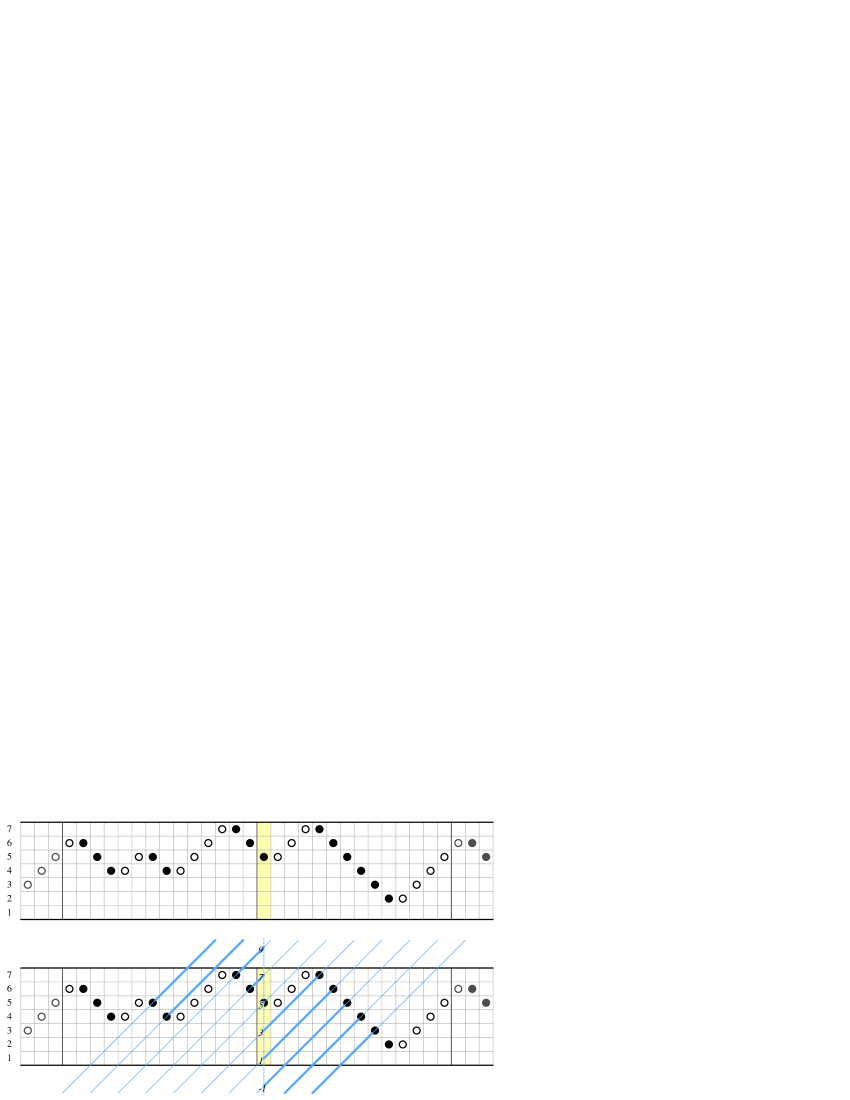
Figure 16: Top: a typical trajectory $h_{t}$, for $L=7$, and $p=28$. Time $t=0$ is at the yellow band. Bottom: illustration of Lemma 5.3, stating that, on the infinite orbit, for all odd values $c$ there exists a unique time $t$ such that $h_{t}-t=c$. Cyan diagonals are the level lines of $g_{t}=h_{t}-t$, at odd values.

The parity statement of Corollary 5.1 has an important consequence.

Lemma 5.2.

Within a periodic portion ${\cal O}^{p}$ of a gyration orbit ${\cal O}$, the number of FPL’s that belong to ${\cal O}^{p}_{+}$, ${\cal O}^{p}_{-}$, ${\cal O}^{p}_{b}$ and ${\cal O}^{p}_{w}$ at any given refinement position $h$ are all equal. In in other words for any function $F$ on $\{1,\ldots,L\}$ and any orbit ${\cal O}$ it holds

$$\sum_{\phi\in{\cal O}^{p}_{+}}F(h(\phi))=\sum_{\phi\in{\cal O}^{p}_{-}}F(h(\phi))=\sum_{\phi\in{\cal O}^{p}_{b}}F(h(\phi))=\sum_{\phi\in{\cal O}^{p}_{w}}F(h(\phi))\,.$$ (62)

Proof.

Fix an orbit ${\cal O}$ and a value $h$. Let $N_{\ast}(h)=|\{\phi\in{\cal O}^{p}_{\ast},\;h(\phi)=h\}|$, for $\ast=+,-,b,w$. We want to prove that $N_{+}(h)=N_{-}(h)=N_{b}(h)=N_{w}(h)$. A consequence of Lemma 5.1 (the fact that $h_{t}-t$ has given parity for configurations in $\mathpzc{Fpl}\!_{b/w}$) is that for $h$ odd $N_{+}(h)=N_{b}(h)$ and $N_{-}(h)=N_{w}(h)$, and for $h$ even $N_{+}(h)=N_{w}(h)$ and $N_{-}(h)=N_{b}(h)$. Call $\{t_{i}\}_{i\in\mathbb{Z}}$ the ordered sequence of times along the orbit such that $h(\phi_{t_{i}})=h$ (say, with $t_{0}$ the first positive value). Clearly $t_{i+N_{b}(h)+N_{w}(h)}=t_{i}+p$. From the discrete continuity properties of $h_{t}$, the configurations $\{\phi_{t_{i}}\}_{i\in\mathbb{Z}}$ are alternating ascending and descending, i.e., as a further consequence of Lemma 5.1, if $\phi_{t_{i}}\in\mathpzc{Fpl}\!_{b}$ then $\phi_{t_{i\pm 1}}\in\mathpzc{Fpl}\!_{w}$, and vice versa. This proves that $N_{b}(h)=N_{w}(h)$, and allows to conclude. ∎

Note that, as an outcome of the construction, we have natural involutions between $\mathpzc{Fpl}\!_{+}$ and $\mathpzc{Fpl}\!_{-}$, and between $\mathpzc{Fpl}\!_{b}$ and $\mathpzc{Fpl}\!_{w}$, which relate FPL’s in the same orbit, preserve the refinement position, and preserve the link pattern up to rotation, e.g. by associating to $\phi(t_{i})\in\mathpzc{Fpl}\!_{b}$ the configuration $\phi(t_{i+1})\in\mathpzc{Fpl}\!_{w}$.

The partition of $\mathpzc{Fpl}\!(\Lambda)$ into orbits is particularly useful when one considers the image of a vector $\mbox{$\|v\rangle\!\rangle$}\in\mathbb{C}^{\mathpzc{Fpl}\!_{+}(\Lambda)}$ under $\mathrm{Sym}\circ\Pi_{+}$, or of a vector $\mbox{$\|w\rangle\!\rangle$}\in\mathbb{C}^{\mathpzc{Fpl}\!_{b}(\Lambda)}$ under $\mathrm{Sym}\circ\Pi_{b}$. Indeed, writing $\|v\rangle\!\rangle$ and $\|w\rangle\!\rangle$ as

$$\|v\rangle\!\rangle =\sum_{{\cal O}}\sum_{\phi\in{\cal O}^{p}_{+}}v(\phi)\mbox{$\|\phi\rangle\!\rangle$}\,; \|w\rangle\!\rangle =\sum_{{\cal O}}\sum_{\phi\in{\cal O}^{p}_{b}}w(\phi)\mbox{$\|\phi\rangle\!\rangle$}\,;$$ (63)

their images under $\mathrm{Sym}\circ\Pi_{+}$ and $\mathrm{Sym}\circ\Pi_{b}$ are simply

$$\mathrm{Sym}\ \Pi_{+}\mbox{$\|v\rangle\!\rangle$} =\sum_{{\cal O}}\Big{(}\sum_{\phi\in{\cal O}^{p}_{+}}v(\phi)\Big{)}\mbox{$|{\cal O}\rangle$}\,; \mathrm{Sym}\ \Pi_{b}\mbox{$\|w\rangle\!\rangle$} =\sum_{{\cal O}}\Big{(}\sum_{\phi\in{\cal O}^{p}_{b}}w(\phi)\Big{)}\mbox{$|{\cal O}\rangle$}\,;$$ (64)

where $\mbox{$|{\cal O}\rangle$}=\mathrm{Sym}\ \Pi_{+}\mbox{$\|\phi\rangle\!\rangle$}$ for any $\phi\in{\cal O}^{p}_{+}$, or also $\mathrm{Sym}\ \Pi_{b}\mbox{$\|\phi\rangle\!\rangle$}$ for any $\phi\in{\cal O}^{p}_{b}$ (these states are well-defined, i.e. do not depend on the choice of $\phi$, because the link pattern is preserved by Wieland gyration, up to rotations).

5.2 Proof of Di Francesco’s 2004 conjecture

Recall that we defined

$$\mbox{$|\Psi_{\Lambda}(t)\rangle$}=\sum_{\phi\in\mathpzc{Fpl}\!_{b}(\Lambda)}t^{h(\phi)-1}\mbox{$|\Pi_{b}(\phi)\rangle$}\,;$$ (65)

as the refinement of the enumerations according to the ‘new’ function $\tilde{\pi}(\phi)=\Pi_{b}(\phi)$. Then let

$$\mbox{$|\Psi^{\prime}_{\Lambda}(t)\rangle$}=\sum_{\phi\in\mathpzc{Fpl}\!_{+}(\Lambda)}t^{h(\phi)-1}\mbox{$|\Pi_{+}(\phi)\rangle$}\,;$$ (66)

the refinement of the enumerations according to the ‘ordinary’ function $\pi(\phi)=\Pi_{+}(\phi)$.

At this point, and at the light of Theorem 4.1, it is easy to restate and prove Di Francesco’s conjecture of [5].

Theorem 5.1 (Di Francesco’s 2004 conjecture).

For any dihedral domain $\Lambda$ and reference side $r$,

$$\mathrm{Sym}\,\mbox{$|\Psi^{\prime}_{\Lambda}(t)\rangle$}=\mathrm{Sym}\,\mbox{$|\Psi_{\Lambda}(t)\rangle$}\,.$$ (67)

More precisely, the original conjecture states that, for $\Lambda$ the $n\times n$ square domain,

$$\mathrm{Sym}\,\mbox{$|\Psi^{\prime}_{\Lambda}(t)\rangle$}=\mathrm{Sym}\,\mbox{$|\Psi^{(1)}_{O(1)}(t)\rangle$}\,.$$ (68)

However, this fact naturally extends to all dihedral domains, up to a proportionality factor, namely $\mathrm{Sym}\,\mbox{$|\Psi^{\prime}_{\Lambda}(t)\rangle$}=K_{\Lambda}(t)\;\mathrm{Sym}\,\mbox{$|\Psi^{(1)}_{O(1)}(t)\rangle$}$, and, at the light of Theorem 4.1 (in the formulation of equation (47)), the restatement in Theorem 5.1 follows.

Proof of Theorem 5.1:  Consider the vectors $\mbox{$\|s^{\prime}_{\Lambda}(t)\rangle\!\rangle$}\in\mathbb{C}^{\mathpzc{Fpl}\!_{+}(\Lambda)}$ and $\mbox{$\|s_{\Lambda}(t)\rangle\!\rangle$}\in\mathbb{C}^{\mathpzc{Fpl}\!_{b}(\Lambda)}$,

$$\|s^{\prime}_{\Lambda}(t)\rangle\!\rangle =\sum_{\phi\in\mathpzc{Fpl}\!_{+}(\Lambda)}t^{h(\phi)-1}\mbox{$\|\phi\rangle\!\rangle$}\,; \|s_{\Lambda}(t)\rangle\!\rangle =\sum_{\phi\in\mathpzc{Fpl}\!_{b}(\Lambda)}t^{h(\phi)-1}\mbox{$\|\phi\rangle\!\rangle$}\,.$$ (69)

Thus $\mbox{$|\Psi^{\prime}_{\Lambda}(t)\rangle$}=\Pi_{+}\mbox{$\|s^{\prime}_{\Lambda}(t)\rangle\!\rangle$}$ and $\mbox{$|\Psi_{\Lambda}(t)\rangle$}=\Pi_{b}\mbox{$\|s_{\Lambda}(t)\rangle\!\rangle$}$. In view of equations (64), and of the decompositions

$$\|s^{\prime}_{\Lambda}(t)\rangle\!\rangle =\sum_{{\cal O}}\sum_{\phi\in{\cal O}^{p}_{+}}t^{h(\phi)-1}\mbox{$\|\phi\rangle\!\rangle$}\,; \|s_{\Lambda}(t)\rangle\!\rangle =\sum_{{\cal O}}\sum_{\phi\in{\cal O}^{p}_{b}}t^{h(\phi)-1}\mbox{$\|\phi\rangle\!\rangle$}\,;$$ (70)

(so that we are in the situation of equations (63)), a sufficient condition for the theorem to hold is that, for all the orbits ${\cal O}$,

$$\sum_{\phi\in{\cal O}^{p}_{+}}t^{h(\phi)-1}=\sum_{\phi\in{\cal O}^{p}_{b}}t^{h(\phi)-1}\,,$$ (71)

which is a special case of Lemma 5.2, with $F(x)=t^{x-1}$. ∎

As a corollary of equation (67) we have the ordinary Razumov–Stroganov correspondence

Corollary 5.2 (Ordinary Razumov–Stroganov correspondence).

The state $|\Psi^{\prime}_{\Lambda}(1)\rangle$ satisfies equation (7).

Proof.

The Wieland Theorem shows that the state $|\Psi^{\prime}_{\Lambda}(1)\rangle$ is rotationally invariant. From the reasonings in Section 2.2 for $|\Psi^{(1)}_{O(1)}(1)\rangle$, and the proportionality of $|\Psi^{(1)}_{O(1)}(1)\rangle$ and $|\Psi_{\Lambda}(1)\rangle$ stated by Theorem 4.1, we already know that $|\Psi_{\Lambda}(1)\rangle$ is the unique solution of equation (7) up to normalisation, and in particular it is rotationally invariant. Thus equation (67) is equivalent to $\mbox{$|\Psi^{\prime}_{\Lambda}(1)\rangle$}=\mbox{$|\Psi_{\Lambda}(1)\rangle$}$, with no need of symmetrisation. As a result, $|\Psi^{\prime}_{\Lambda}(1)\rangle$ satisfies equation (7). ∎

5.3 A bijection between $\mathpzc{Fpl}\!_{+}(\Lambda)$ and $\mathpzc{Fpl}\!_{b}(\Lambda)$

In the previous paragraphs we have introduced bijections between $\mathpzc{Fpl}\!_{+}$ and $\mathpzc{Fpl}\!_{-}$, and between $\mathpzc{Fpl}\!_{b}$ and $\mathpzc{Fpl}\!_{w}$, which relate FPL’s in the same orbit, preserve the refinement position, and preserve the link pattern up to rotation.

In this section we introduce an explicit bijection between $\mathpzc{Fpl}\!_{+}(\Lambda)$ and $\mathpzc{Fpl}\!_{b}(\Lambda)$, which relates FPL’s within the same orbit, and preserves the link pattern, when produced with $\Pi_{+}$ and $\Pi_{b}$ respectively (but does not preserve the refinement position).

This bijection allows to recover the ordinary Razumov–Stroganov correspondence based on fully-packed loop configurations in $\mathpzc{Fpl}\!_{+}(\Lambda)$, from the central theorem proven in this paper, Theorem 4.1, without using Theorem 5.1, nor the results in [6].

Roughly speaking, the idea is to rotate a FPL $\phi\in\mathpzc{Fpl}\!_{+}(\Lambda)$ until the image of the external edge with label $1$ coincides with the refinement position. While a priori it is not obvious that this event ever occurs within the orbit, this fact is ensured by the following

Lemma 5.3.

The function $g_{t}=h_{t}-t$ is non-increasing, and each odd value has exactly one preimage.

Proof.

The proof is a simple consequence of the table in Lemma 5.1, which implies that if $g_{t}$ is even, then $g_{t+1}\in\{g_{t},g_{t}-1\}$, and if $g_{t}$ is odd, then $g_{t+1}\in\{g_{t}-2,g_{t}-1\}$. The idea is also illustrated in Figure 16, bottom. ∎

This lemma provides the claimed bijection. For the orbit with $\phi_{0}=\phi$, call $t^{*}(\phi)$ the preimage of $1$ under $g_{t}$ (which is unique from the lemma). Then we have

Proposition 5.1.

We have a bijection $\Theta:\mathpzc{Fpl}\!_{+}(\Lambda)\rightarrow\mathpzc{Fpl}\!_{b}(\Lambda)$, defined, together with its inverse, as

$$\Theta(\phi) :=H^{t^{*}(\phi)}\phi\,; \Theta^{-1}(\phi) :=H^{-h(\phi)+1}\phi\,.$$ (72)

Furthermore, $\Pi_{+}(\phi)=\Pi_{b}(\Theta(\phi))$.

Proof.

The fact that $\Pi_{+}(\phi)=\Pi_{b}(\Theta(\phi))$ is a restatement of $g_{t}=1$ (at the light of the fact that each half-gyration rotates the link pattern one position counter-clockwise).

The fact that $\Theta(\Theta^{-1}(\phi))=\phi$, as defined in (72), follows from the definition of $t^{*}(\phi)$. The fact that also $\Theta^{-1}(\Theta(\phi))=\phi$, follows by observing that $0=h_{t^{*}(\phi)}-t^{*}(\phi)-1=h(\Theta(\phi))-t^{*}(\phi)-1$, that is, $(H^{t^{*}(\phi)})^{-1}=H^{-(h(\Theta(\phi))-1)}$. ∎

Using the statement $\Pi_{+}(\phi)=\Pi_{b}(\Theta(\phi))$, we can easily show that $\mbox{$|\Psi^{\prime}_{\Lambda}(1)\rangle$}=\mbox{$|\Psi_{\Lambda}(1)\rangle$}$:

$$\mbox{$|\Psi^{\prime}_{\Lambda}(1)\rangle$}=\Pi_{+}\!\!\sum_{\phi^{\prime}\in\mathpzc{Fpl}\!_{+}(\Lambda)}\!\!\mbox{$\|\phi^{\prime}\rangle\!\rangle$}=\Pi_{b}\!\!\sum_{\phi^{\prime}\in\mathpzc{Fpl}\!_{+}(\Lambda)}\!\!\mbox{$\|\Theta(\phi^{\prime})\rangle\!\rangle$}=\Pi_{b}\!\!\sum_{\phi\in\mathpzc{Fpl}\!_{b}(\Lambda)}\!\!\mbox{$\|\phi\rangle\!\rangle$}=\mbox{$|\Psi_{\Lambda}(1)\rangle$}\,.$$ (73)

Through Theorem 4.1, this is another proof of the Razumov–Stroganov correspondence.

References

- Bax [82] R.J. Baxter, Exactly solved models in Statistical Mechanics, Academic Press, London, 1982
- Bre [99] D.M. Bressoud, Proofs and Confirmations — The Story of the Alternating-Sign Matrix Conjecture, Cambridge Univ. Press, 1999
- CS [10] L. Cantini and A. Sportiello, Proof of the Razumov-Stroganov conjecture, Journ. of Comb. Theory A118 1549-1574 (2011) arXiv:1003.3376
- [4] L. Cantini and A. Sportiello, FPL domains with dihedral symmetry and generalized Razumov–Stroganov correspondence, in preparation.
-
[5]
P. Di Francesco,
A refined Razumov–Stroganov conjecture,
J. Stat. Mech. P08009 (2004)
arXiv:cond-mat/0407477 - DZ [04] P. Di Francesco and P. Zinn-Justin, Around the Razumov–Stroganov conjecture: proof of a multi-parameter sum rule, Elect. J. Comb. 12 R6 (2005) arXiv:math-ph/0410061
-
DZZ [06]
P. Di Francesco, P. Zinn-Justin and J.-B. Zuber,
Sum rules for the ground states of the loop model on a
cylinder and the XXZ spin chain,
J. Stat. Mech. P08011 (2006)
arXiv:math-ph/0603009 - Duc [07] Ph. Duchon, On the link pattern distribution of quater-turn symmetric FPL configurations, in Proc. of FPSAC 2008, Valparaiso (Chile), 2008 arxiv:math.CO/0711.2871
- Ize [87] A. Izergin, Partition function of the six-vertex model in a finite volume, Sov. Phys. Dokl. 32 878-879 (1987)
- Kup [96] G. Kuperberg, Another proof of the alternating sign matrix conjecture, Intern. Math. Res. Notes 1996(3) 139-150 (1996), arXiv:math.CO/9712207
- Kup [00] G. Kuperberg, Symmetry classes of alternating-sign matrices under one roof, Ann. of Math. 156 (2002) 835-866 arXiv:math/0008184
- [12] A.V. Razumov and Yu.G. Stroganov, Combinatorial nature of ground state vector of loop model, Theor. Math. Phys. 138 333-337 (2004) [russian: Teor. Mat. Fiz. 138 395-400 (2004)] arXiv:math/0104216
- [13] A.V. Razumov and Yu.G. Stroganov, loop model with different boundary conditions and symmetry classes of alternating-sign matrices, Theor. Math. Phys. 142 237-243 (2005) [russian: Teor. Mat. Fiz. 142 284-292 (2005)] arXiv:cond-mat/0108103
- Wie [00] B. Wieland, Large Dihedral Symmetry of the Set of Alternating Sign Matrices, Elect. J. Comb. 7 R37 (2000), arXiv:math/0006234
-
Zei [94]
D. Zeilberger,
Proof of the alternating sign matrix conjecture,
Elect. J. Comb. 3 R13 (1996)
arXiv:math/9407211 - Zei [96] D. Zeilberger, Proof of the refined alternating sign matrix conjecture, New York J. Math. 2 59-68 (1996) arXiv:math/9606224
- [17] P. Zinn-Justin, Six-Vertex, Loop and Tiling models: Integrability and Combinatorics, HDR thesis, LAP Lambert Academic Publishing, 2010, arXiv:0901.0665