X-ray Monitoring of Gravitational Lenses With Chandra

Abstract

We present Chandra monitoring data for six gravitationally lensed quasars: QJ 0158$-$4325, HE 0435$-$1223, HE 1104$-$1805, SDSS 0924+0219, SDSS 1004+4112, and Q 2237+0305. We detect X-ray microlensing variability in all six lenses with high confidence. We detect energy dependent microlensing in HE 0435$-$1223, SDSS 1004+4112, SDSS 0924+0219 and Q 2237+0305. We present a detailed spectral analysis for each lens, and find that simple power-law models plus Gaussian emission lines give good fits to the spectra. We detect intrinsic spectral variability in two epochs of Q 2237+0305. We detect differential absorption between images in four lenses. We also detect the Fe K$\alpha$ emission line in all six lenses, and the Ni XXVII K$\alpha$ line in two images of Q 2237+0305. The rest frame equivalent widths of the Fe K$\alpha$ lines are measured to be 0.4–1.2 keV, significantly higher than those measured in typical active galactic nuclei of similar X-ray luminosities. This suggests that the Fe K$\alpha$  emission region is more compact or centrally concentrated than the continuum emission region.

1 Introduction

The concept of quasar microlensing, the effect of gravitational lensing by stellar mass objects in a lens galaxy on background quasars, was proposed almost immediately (e.g., Chang & Refsdal 1979; Gott 1981) after the discovery of the first gravitational lens (Walsh et al. 1979). However, it was only ten years later that the effect was observationally detected in Q 0957+561 (Vanderriest et al. 1989) and Q 2237+0305 (Irwin et al. 1989). Recently, quasar microlensing has become an important tool for probing the structure of quasar accretion disks and distinguishing models for their non-thermal emission (see the reviews by Wambsganss 2006; Kochanek et al. 2007). The ensemble of microlensing stars produces a magnification pattern in the source plane, and as the source moves across this pattern due to relative motions between the source, the lens, the stars in the lens, and the observer, the source magnification varies with time. More importantly for studying accretion disk models, the (time varying) microlensing magnification depends on the size and spatial structure of the emission source in the central engine of quasar. Larger emission regions smooth the magnification patterns more heavily and will have less microlensing variability than smaller emission regions. Additionally, the magnification diverges on caustics, which makes it possible to resolve emission regions arbitrarily smaller than the Einstein radius of the stars. Unlike almost any other astrophysical probe, microlensing becomes a more powerful tool as the source becomes smaller. As a result, quasar microlensing is a unique tool for probing the innermost structure of accretion disks.

There are two major challenges in utilizing this approach: first, to measure the microlensing light curves and second, to interpret the curves. There are several effects contributing to the light curves of quasar images and their variability. First, the average fluxes of the images are affected by the macro lens model, milli-lensing by substructures in the lens (e.g., Kochanek & Dalal 2004; Cohn & Kochanek 2004; Keeton & Moustakas 2009), extinction by dust (e.g., Falco et al. 1999; Elíasdóttir et al. 2006), and X-ray absorption by gas in the lens (e.g., Dai et al. 2006; Dai & Kochanek 2009). Second, they vary with time due to a combination of microlensing and the intrinsic variability of quasars. Of these effects, the intrinsic variability is usually relatively easy to remove by measuring the time delays between the images and then shifting the light curves. Many of other effects are also energy/wavelength dependent, but the best way to distinguish microlensing variability from other effects is through long term monitoring programs at the relevant energies. This approach also has the advantages of ameliorating systematic uncertainties due to the mean stellar mass in the lens galaxy. Limited by observational resources, early microlensing studies were confined to either single epoch, multiple wavelength (e.g., Falco et al. 1996; Mediavilla et al. 1998; Agol et al. 2000), or multiple epoch, single wavelength studies (e.g., Wo$\acute{\rm{z}}$niak et al. 2000). Only recently have there been intensive studies spanning both the time and wavelength (e.g., Poindexter et al. 2008; Chen et al. 2011; Blackburne et al. 2011; Mosquera et al. 2011; Mu$\rm\tilde{n}$oz et al. 2011).

Theoretically, the importance of the clustering of caustics on interpretation of quasar microlensing light curves was realized quite early (e.g., Wambsganss et al. 1990). Because of the high optical depth of quasar microlensing in lens systems, quasar microlensing light curves are generally affected by many stars, thus requiring theoretical models constructed for these complicated conditions. The only real solution has been to simply model the data using variants of the Bayesian Monte Carlo method (Kochanek 2004). This technique and its variants have led to unique constraints on the emission sizes of accretion disks in different wavelengths (Morgan et al. 2008; Eigenbrod et al. 2008; Chartas et al. 2009; Dai et al. 2010; Mediavilla et al. 2011, Poindexter & Kochanek 2010b; Blackburne et al. 2011), and on the stellar/dark matter distribution of the foreground lensing galaxies (e.g., Mediavilla et al. 2009; Poindexter & Kochanek 2010a; Bate et al. 2011; Pooley et al. 2012).

We are particularly interested in using microlensing to study the non-thermal, X-ray emission regions of quasar accretion disks. The X-ray continuum emission of quasars is observed to follow a power-law, and it is believed to be generated through the unsaturated inverse Compton scattering of UV disk photons on hot electrons in a corona above the disk (see the review by Reynolds & Nowak 2003). The origin of the corona, its geometrical size and detailed structure are still topics under debate. In addition to the X-ray continuum, the disk-corona model also predicts the existence of a reflection component including emission lines (e.g., Fe K$\alpha$) formed through irradiation of the colder accretion disk by the continuum (e.g., George & Fabian 1991). However, the location of this reflection component, whether it comes from the disk, the disk-wind, or the “torus”, has been debated for more than two decades. In principle, with enough observations, the quasar microlensing technique can resolve all these issues.

Microlensing of X-rays was first tentatively suggested in RX J0911.4+0551 (Morgan et al. 2001). Because of the lack of multi-epoch observations and the large intrinsic X-ray variability in quasars, later studies focused on microlensing of the Fe K$\alpha$ line (Chartas et al. 2002, 2004; Dai et al. 2003; Ota et al. 2006), where dramatic changes in the Fe K$\alpha$ line equivalent widths were most easily interpreted. Studies of the X-ray continuum resumed with the report of the dramatic flux ratio differences between the X-ray and optical bands in RXJ1131$-$1231 (Blackburne et al. 2006) and the single epoch, optical-to-X-ray flux ratio comparison for a sample of lenses by Pooley et al. (2006). Short Chandra monitoring programs of a few lenses start to emerge at this stage (e.g., Chartas et al. 2009), and combining them with the Bayesian Monte Carlo microlensing analysis technique (Kochanek 2004), we have generally found that the X-ray continuum is emitted on scales of roughly $10\,r_{g}$ (Morgan et al. 2008; Chartas et al. 2009; Dai et al. 2010; Blackburne et al. 2011), 7–10 times smaller than the observed optical emission region (Morgan et al. 2010). However, the current lower limits on the sizes of the X-ray emission regions are not well constrained, because strong lower limits require more densely sampled light curves than any presently available. Nonetheless, these microlensing results have ruled out disk-corona models where the corona covers extensive areas of the optical accretion disk. The large equivalent widths of the Fe K$\alpha$ line measured in a few lensed quasars suggest that a significant fraction of the Fe K$\alpha$ line flux originates from a region smaller than the X-ray continuum emission region (Dai et al. 2003; Popovi$\rm\acute{c}$ et al. 2003, 2006). However, these studies were limited by the lack of deep, better sampled X-ray microlensing light curves.

In this paper, we report results from monitoring six gravitationally lensed quasars with Chandra: QJ 0158$-$4325 (Maza et al. 1995; Morgan et al. 1999), SDSS 0924+0219 (Inada et al. 2003a), SDSS 1004+4112 (Inada et al. 2003b), HE 0435$-$1223 (Wisotzki et al. 2002), HE 1104$-$1805 (Wisotzki et al. 1993), and Q 2237+0305 (Huchra et al. 1985). This is the largest quasar microlensing X-ray monitoring program to date. QJ 0158$-$4325 and HE 1104$-$1805 are doubly imaged while the other four systems have four bright images. Five of the foreground lenses are galaxies, while SDSS 1004+4112 is lensed by a galaxy cluster. Since microlensing in the optical bands has been extensively studied in these systems (e.g., Morgan et al. 2006; Kochanek et al. 2006; Lamer et al. 2006; Fohlmeister et al. 2007, 2008; Eigenbrod et al. 2008; Faure et al. 2009; Poindexter & Kochanek 2010a, 2010b; Ricci et al. 2011; Blackburne et al. 2011), our X-ray microlensing light curves provide complementary data to constrain non-thermal emission processes in accretion disks. For example, a simple comparison of the microlensing variability between the soft and the hard X-ray bands in Q 2237+0305 has already led us to conclude that the hard X-ray continuum emission region is smaller than that of the soft in this quasar, suggesting a temperature gradient in the X-ray emitting corona (Chen et al. 2011). In our original proposals, only the observations of Q 2237+0305 and RXJ1131$-$1231 (which will be discussed in Chartas et al. 2012) were explicitly designed to have the count rates needed to obtain accurate measurements in multiple energy bands.

We present the Chandra observations and the data reduction techniques in Section 2, the image analysis in Section 3, and the spectral analysis in Section 4. The microlensing analysis is in Section 5, and the discussion and conclusions in Section 6. Throughout this paper, we assume a flat $\Lambda$CDM cosmology with $\Omega_{\Lambda}=0.73,$ $\Omega_{M}=0.27,$ and $\rm H_{0}=70\,km\,s^{-1}\,Mpc^{-1}.$

2 Observations And Data Reduction

All observations presented in this paper were made with ACIS (Garmire et al. 2003) on the Chandra X-ray Observatory (Weisskopf et al. 2002). With an on-axis point spread function (PSF) of 0${}^{\prime\prime}\!\!.$5, Chandra is the only X-ray telescope that can resolve lensed images typically separated by 1–2^′′. The majority of the observations are from our large Chandra Cycle 11 program to monitor seven gravitational lenses. Here, we report on six of the lenses, QJ 0158$-$4325, SDSS 0924+0219, SDSS 1004+4112, HE 0435$-$1223, HE 1104$-$1805, and Q 2237+0305. Although the absorption corrected count rates of Q 2237+0305 were published in Chen et al. (2011), we present the detailed spectral analysis in this paper. The analysis of RXJ1131$-$1231 will be presented in a companion paper (Chartas et al. 2012, in preparation). We also analyzed the archival Chandra data for the six lenses. We list the basic information for these observations, such as observation dates and exposure times, in Tables 1$-$6.

We reprocessed all data using the CIAO 4.3 software tools by first removing the pixel randomization and applying a sub-pixel algorithm for event positions (Tsunemi et al. 2001). We then filtered all events using the standard ASCA grades of 0, 2, 3, 4 and 6 with energies between 0.4 and 8.0 keV (observer’s frame), and further separated the events into soft and hard bands for subsequent analyses. We selected the energy boundary between the soft and hard band for each lensing system to balance the soft and hard band count rates (see e.g., Table 1) in order to produce the best statistics for detecting differences between the two energy bands. For QJ 0158$-$4325, SDSS 0924+0219, and SDSS 1004+4112 we split the soft and hard bands at 3.0 keV (rest frame), for HE 0435$-$1223 and Q 2237+0305 we split the soft and hard bands at 3.5 keV (rest frame), and for HE 1104$-$1805, we split the soft and hard bands at 4.0 keV (rest frame). In Chen et al. (2011), we used (observed frame) full, soft, and hard bands at 0.2–8.0 keV, 0.2–2.0 keV, and 2.0–8.0 keV respectively. In the current paper, we define the full band as 0.4–8.0 keV, and divide the soft and hard bands at 1.3 keV (3.5 keV in rest frame). This energy division provides better statistical results than our definitions in Chen et al. (2011), but it alters none of our conclusions. The pile-up effect is negligible for all our sources ($<$2% in all images), since they are generally faint. Nevertheless, we used the 1/2 subarray mode in our observations of QJ 0158$-$4325, SDSS 0924+0219, HE 0435$-$1223, HE 1104$-$1805, and Q 2237+0305 in order to minimize any residual pile-up effects. In our program, RXJ1131$-$1231 is the only case where the pile-up effect needs to be extensively modeled (Chartas et al. 2009).

3 Imaging Analysis

Beside the cluster lens SDSS1004+4112, whose four bright images are well separated from each other (Inada et al. 2003b), the images in the five galaxy-scale lenses are separated by only 1–2 arcsec and their PSFs are therefore blended. In each of these systems, we first extracted the total counts in each band (full, soft, and hard) within circular apertures 3–$4^{\prime\prime}$ in radius that contain most of the source counts (see Figure 1). We estimated the background using concentric annular regions with inner and outer radii of $\sim$$10^{\prime\prime}$ and $\sim$$20^{\prime\prime}$, respectively. We then used PSF fitting to model the relative count rates between the images, fixing the relative image positions to the HST positions from the CASTLES website. We binned the X-ray images in 0${}^{\prime\prime}\!\!.$0984 pixels, and fit these binned images using Sherpa to minimize the Cash C-statistic between the observed and model images. The count rates were then normalized by partitioning the background-subtracted total source counts based on the relative count rates for each image obtained from the PSF fits. Although some images in these five lenses are well-separated and their count rates could also be estimated using aperture photometry, we find that the count rates from the two methods are consistent and report only the results based on the PSF fits.

In SDSS 1004+4112, the four images are well separated (from $\sim$$4^{\prime\prime}$ to $\sim$$15^{\prime\prime}$), so we computed the photon count rates using aperture photometry. Since the foreground lens is a cluster, there is non-negligible X-ray emission from the cluster at the positions of the lensed images (Ota et al. 2006). We chose a circular region of $\sim$1${}^{\prime\prime}\!\!.$5 radius around each image as the source region. We estimated the local background in partial annuli at the same radius from the cluster center as the quasar images in order to estimate, and then subtract the contamination from the lensing cluster. We then corrected for the finite aperture size to determine the total count rates in Table 4.

In all six lenses, the count rate of each image was corrected for Galactic absorption and absorption in the lens (see Section 4). The final results are presented in Tables 1–6. We note that the total count rates can differ slightly from the sum of the soft and hard band count rates because the PSF fits were done separately for the full, soft, and hard band images, and because of the absorption corrections. Finally, we also constructed a stacked image (combining all epochs) using the best-fitting image positions obtained from the fits to register the epochs and then smoothing with a suitably sized Gaussian kernel. These images are shown in Figure 1.

4 Spectral Analysis

We extracted three sets of spectra from each lens: the spectra of the individual images for the individual epochs, the stacked spectra of the individual images combining all the epochs, and the stacked spectra of all images. First, we extracted spectra of the individual images using the CIAO tool “psextract” in circles of radii about 0${}^{\prime\prime}\!\!.$5–0${}^{\prime\prime}\!\!.$8 (for SDSS 1004+4112 we used 1${}^{\prime\prime}\!\!.$5) centered on the positions from the PSF fits to each observation. Because of the superb angular resolution of Chandra, the normal X-ray background contributes little to the source spectrum, and the “background” is dominated by contaminating emission from adjacent images. To estimate the contamination of image A by image B, we measured the spectrum in a circular aperture of the same size at the position X that A would have if reflected through image B (i.e., X$-$B$-$A with $\rm\overline{XB}=\overline{BA}$). For the cluster lens SDSS 1004+4112, we extracted the source spectra using 1${}^{\prime\prime}\!\!.$5 radius apertures and the background spectra from concentric partial rings at the same radius from the cluster center to model the cluster contamination. Images C and D of SDSS 0924+0219 are faint and poorly resolved (see Figure 1), so we extracted a single spectrum from a polygonal region containing images A, C and D. After extracting the spectra of the individual images for each epoch, we also obtained combined spectra for each image by stacking the spectra from the different epochs and the corresponding rmf and arf files weighted by their exposure times to increase the S/N ratio of the spectra. Finally, we obtained a spectrum combining all the images and all the epochs for each lens.

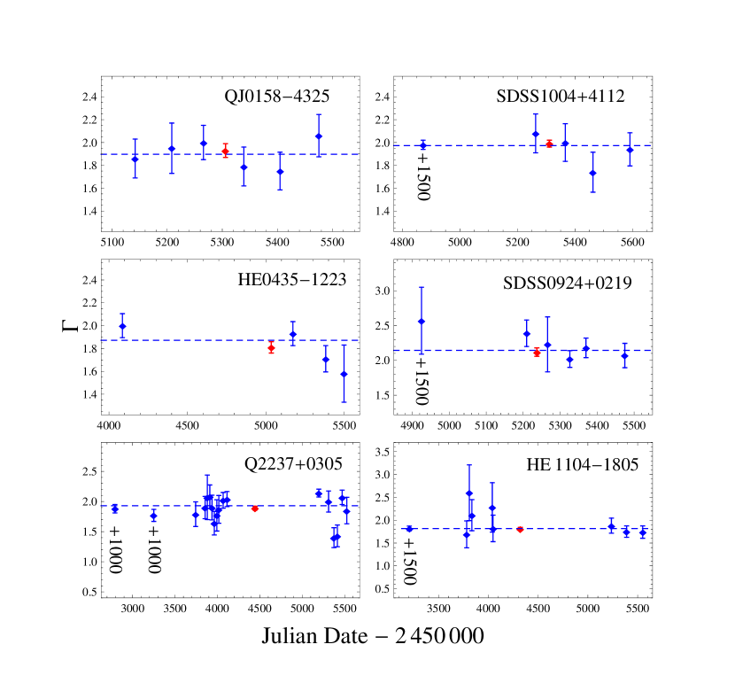
Figure 2: Evolution of the spectral power-law index $\Gamma$ with time for QJ 0158$-$4325, SDSS 0924+0219, HE 0435$-$1223, SDSS 1004+4112, Q 2237+0305 and HE 1104–1805. For clarity, the first points for SDSS 0924+0219, SDSS 1004+4112 and HE 1104–1805 are shifted by +1500 days, and the first two events of Q 2237+0305 are shifted by +1000 days. In each panel, the dashed horizontal line is the best fit $\Gamma$ to the measurements from the individual epochs, and the red point is the power-law index $\Gamma$ obtained from fitting the stacked spectra.

We analyzed the spectra using XSPEC V12. We first modeled the spectra of the individual images extracted from the individual epochs using a simple power-law model modified by Galactic absorption (Dickey & Lockman 1990) and neutral absorption at the lens over the 0.4–8.0 keV band. In the fitting process, we assumed the same fixed Galactic absorption for all the images of a lens, but allowed the absorption from the lens galaxy to vary independently. We further assumed that the power-law index $\Gamma$ of the source spectrum was the same for all images. In general, this may not be true either because of the intrinsic spectral variability modulated by the time delays between the images, or because of energy-dependent microlensing, but it is a good average approximation. The spectral fitting results are presented in Tables 7–12, and Figure 2 shows the evolution of the power-law index $\Gamma$ in each lens. Besides the power-law index $\Gamma$ and the column density $\rm N_{H}$ of the neutral absorption in the lens, we also give the estimated absorption-corrected energy flux for the soft and hard bands.

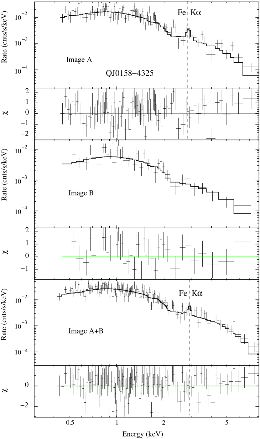
Figure 3: Stacked spectra of QJ 0158$-$4325 (observed frame) fit with a simple power-law plus Gaussian line model modified by Galactic and lens galaxy absorption. The top, middle, and bottom panels show results for image A, image B, and their combined spectrum, in each case showing the data and the model fit in one sub-panel, and the statistical residuals in a second sub-panel.

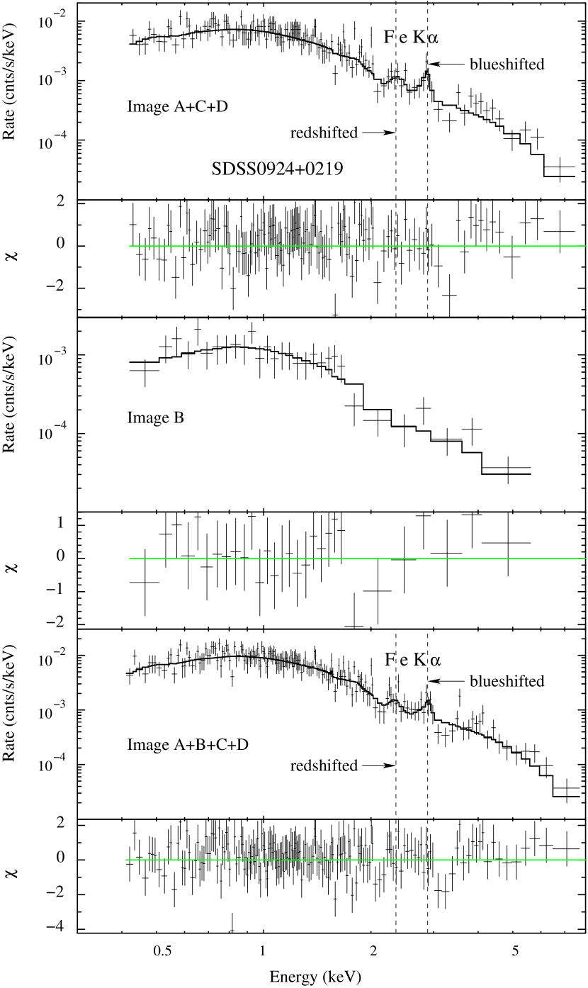
Figure 4: Stacked spectra of SDSS 0924+0219 (observed frame) fit with a simple power-law plus Gaussian line model modified by Galactic and lens galaxy absorption. The top, middle, and bottom panels show results for image A+C+D, image B, and their combined spectrum, in each case showing the data and the model fit in one sub-panel, and the statistical residuals in a second sub-panel. We detect both a blueshifted and a redshifted wing of the iron line.

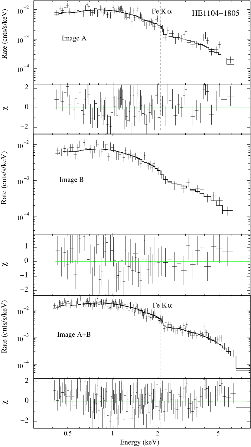
Figure 5: Stacked spectra of HE 1104$-$1805 (observed frame) fit with a simple power-law plus Gaussian line model modified by Galactic and lens galaxy absorption. The top, middle, and bottom panels show results for image A, image B, and their combined spectrum, in each case showing the data and the model fit in one sub-panel, and the statistical residuals in a second sub-panel.

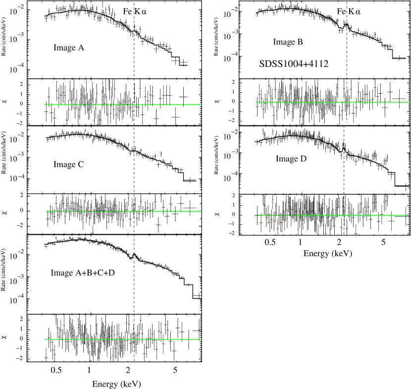
Figure 6: Stacked spectra of SDSS 1004+4112 (observed frame) fit with a simple power-law plus Gaussian line model modified by Galactic and lens galaxy absorption. The individual A, B, C, and D spectra as well as the stacked A+B+C+D spectrum are shown, in each case showing the data and the model fit in one sub-panel, and the statistical residuals in a second sub-panel.

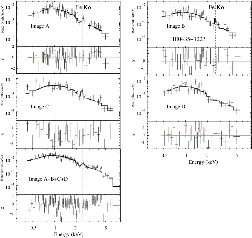
Figure 7: Stacked spectra of HE 0435$-$1223 (observed frame) fit with a power-law plus Gaussian line model modified by Galactic and lens galaxy absorption. The individual A, B, C, and D spectra as well as the stacked A+B+C+D spectrum are shown, in each case showing the data and the model fit in one sub-panel, and the statistical residuals in a second sub-panel.

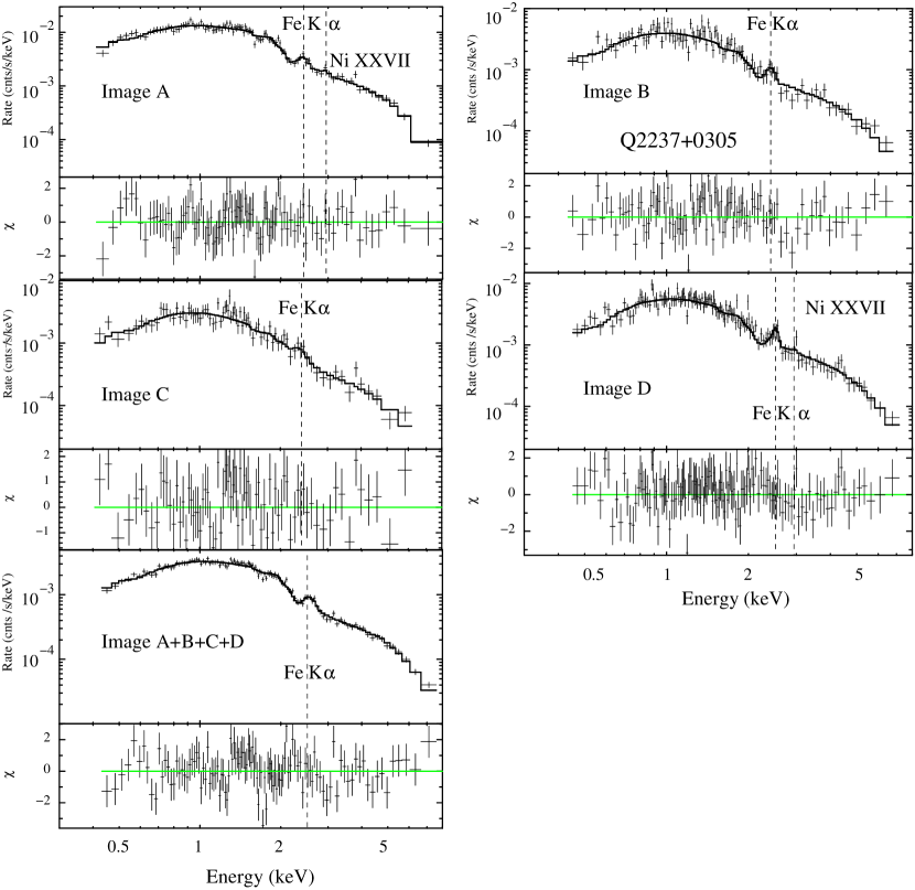
Figure 8: Stacked spectra of Q 2237+0305 (observed frame) fit with a simple power-law plus Gaussian line model modified by Galactic and lens galaxy absorption.The individual A, B, C, and D spectra as well as the stacked A+B+C+D spectrum are shown, in each case showing the data and the model fit in one sub-panel, and the statistical residuals in a second sub-panel. Iron line is detected in images A, B, C and D. The nickel line is only detected in images A and D.

To better constrain the lens absorption and power-law indices of the quasar, we fit the stacked spectra combining the individual epochs for each image. These spectra are shown in Figures 3–8. When fitting these stacked spectra, we also added Gaussian emission lines to the model. We detected differential absorption between some of the images in all the lenses except for SDSS 0924+0219 and HE 1104$-$1805. We detected Fe K$\alpha$ emission lines in all lenses and the Ni XXVII K$\alpha$ line in Q 2237+0305. We list the spectral fitting results for the stacked spectra in Tables 7–12 for the photon indices and lens absorption and in Table 13 for the emission lines. After obtaining the best fits to the stacked spectra, we calculated the ratios of the count rates between the absorbed and unabsorbed models in the full, soft, and hard bands, respectively. These mean ratios were then applied to the absorbed count rates of the individual epochs and images to estimate the absorption corrected count rates. For SDSS 0924+0219 we use the same absorption correction for images A, C and D. We also modeled the stacked spectra allowing different power-law indices between the images. Finally, we fit the stacked spectrum combining all images and all epochs for each lens, and these results are also presented in Tables 7–12.

4.1 Photon Indices

We show the time evolution of the power-law index $\Gamma$ of each lens in Figure 2. To test for spectral variability, we can compare the fits to the individual epochs to their mean and its uncertainty (dashed lines in Figure 2). The results for QJ 0158$-$4325, HE 0435$-$1223, HE 1104$-$1805, SDSS 0924+0219, and SDSS 1004+4112 are all consistent with a constant spectral index. Only Q 2237+0305 shows clear evidence for spectral variability, with a constant $\Gamma$ model having $\chi^{2}=38.4$ (dof=17), so we detect spectral variability in Q 2237+0305 at $99.8\%$ confidence. This spectral variability is mainly caused by epochs 15 and 16, where the power-law index drops suddenly from $\sim$$2.0$ to $\sim$$1.4$. These two epochs contribute $\sim$$18.0$ out of the total $\chi^{2}=38.4$, and the spectral variability would not be statistically significant without these two points.

Spectral variability can be either intrinsic variability or caused by chromatic microlensing between the soft and hard X-ray bands. For example, the spectrum of a microlensed quasar image more strongly magnified in the hard X-ray band will appear harder than the other images. Distinguishing these two possibilities is particularly important for Q 2237+0305, since in this lens we observed more microlensing variability amplitude in the hard X-ray band than in the soft. As can be seen from Figures 2 and 3 of Chen et al. (2011), around date 5400 (epochs 15 and 16), there is no significant microlensing variability in images A, B, and D based on the relatively flat B/A, D/A, and B/D flux ratio light curves. Although there appears to be some microlensing activity in image C around this time, image C is the faintest of the four images at this time and contributes less than $10\%$ of the total flux (Table 12, fit No. 15, 16), so it cannot be responsible for the sudden decrease in the power-law index. Moreover, if we fit the spectra of the four images independently at these two epochs, we find similar photon indices for all images. We conclude that the spectral variability at these two epochs is intrinsic, instead of due to chromatic microlensing. We also compare the average power-law indices of the individual epochs (dashed lines in Figure 2) with those obtained from fitting the stacked spectra combining all the epochs (red points in Figure 2), and find that they are consistent.

4.2 Absorption in the Lens

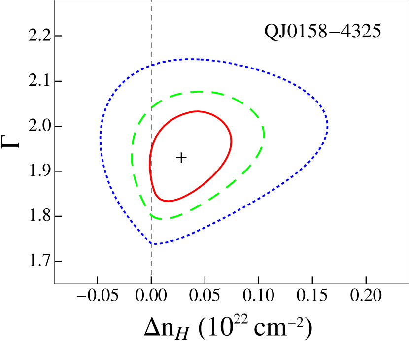
Figure 9: Differential absorption $\rm n_{H}^{B}-n_{H}^{A}$ in the lens as a function of the power-law index $\Gamma$ for QJ 0158$-$4325. The stacked spectra of image A and B are simultaneously fit with the same power-law index but different amounts of neutral absorption $n_{H}.$ The red solid, green dashed, and blue dotted curves show the two-parameter $68\%,$ $90\%$ and $99\%$ confidence contours respectively.

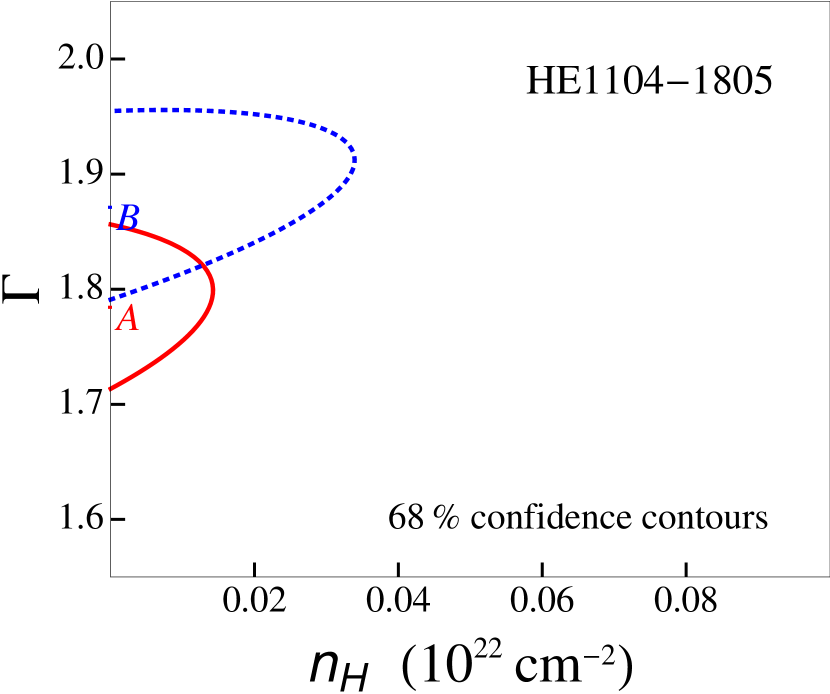
Figure 10: Lens absorption $\rm n_{H}$ as a function of the power-law index $\Gamma$ for HE 1104–1805. The curves show the 68% confidence level contour for two parameters.

We report our estimates for the amount of absorption in the lens from analyzing the combined spectra of each image in Tables 7–12 (the $5^{\rm th}$ column). For absorption we focus on the stacked spectra since the changes in the intrinsic spectra are small or non-existent and the absorption does not change between epochs. The stacked spectra of QJ 0158$-$4325, SDSS 0924+0219, HE 1104$-$1805, SDSS 1004+4112, HE 0435$-$1223, and Q 2237+0305 are shown in Figures 3–8 along with their best-fit models (a power-law modified by Galactic and lens absorption plus Gaussian emission lines). Figures  9–11 show the two-parameter confidence contours for the estimated column densities $\rm N_{H}$ and the spectral index $\Gamma$ of the source. For the two-image lens QJ 0158–4325, we detect differential absorption between image A and B (Figure 9). We detect no lens absorption in HE 1104$-$1805 (Figure 10). For SDSS 0924+0219, images C and D are not well separated from image A, so we extracted only one spectrum combining images A, C and D, labeled by ACD in Figure 11 (bottom right panel). We detected no neutral absorption in SDSS 0924+0219. We detected differential absorption between images in SDSS 1004+4112, HE 0435–1223, and Q 2237+0305. Dai et al. (2003) detected neutral absorption in images A and C of Q 2237+0305, but not in images B and D (see also Agol et al. 2009). The latest Chandra data (stacking over 20 epochs with a total exposure time over 290 ks) shows that there is neutral absorption in all 4 images, where image D suffers the most significant absorption from the foreground lens.

4.3 Metal Emission Lines

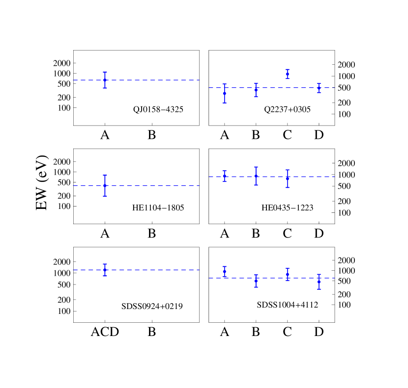
Figure 12: Rest frame equivalent widths of the Fe K$\alpha$  lines of QJ 0158$-$4325, Q 2237+0305, HE 1104$-$1805, HE 0435$-$1223, SDSS 0924+0219, and SDSS 1004+4112. Dashed lines are the best fits for the equivalent widths of the images as constants. For SDSS 0924+0219, we extracted one spectrum for the combination of images A, C, and D, and the iron line for this spectra is labeled by $\rm ACD$ (A is the brightest image). The iron line was detected in all four images of SDSS 1004+4112, and Q 2237+0305. We did not detect the iron line in image B of QJ 0158$-$4325, SDSS 0924+0219, or HE 1104$-$1805, or image D of HE 0435$-$1223.

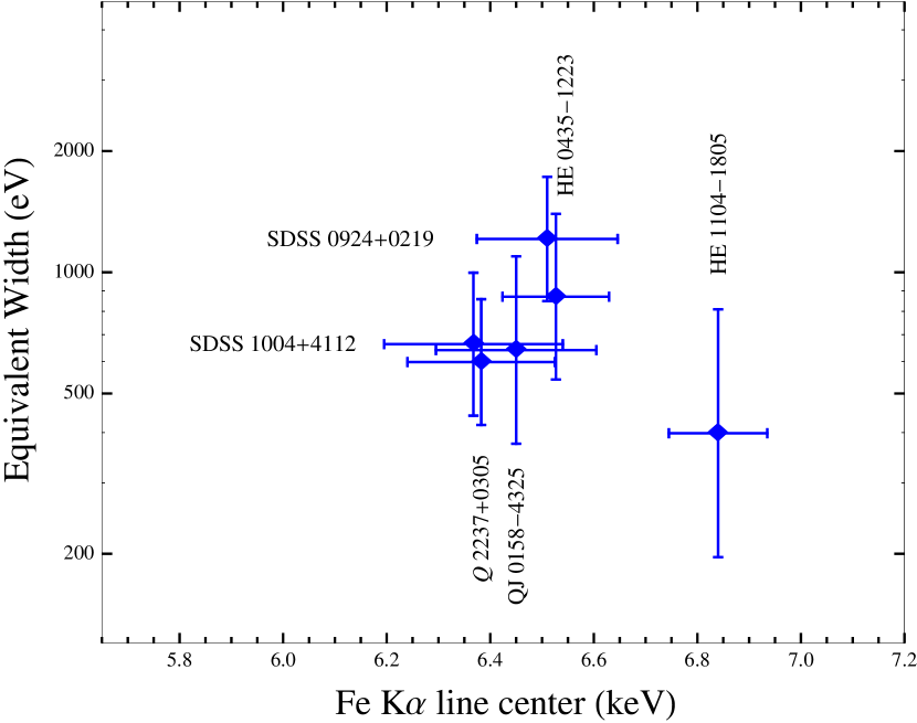
Figure 13: Average rest frame Fe K$\alpha$  line centers and equivalent widths for the six lenses.

We detect Fe K$\alpha$ emission lines in all six lenses. Table 13 reports the rest frame mean energy, $\rm E_{line},$ Gaussian line width, $\sigma_{\rm line},$ the equivalent width, EW, and significance for each lens. Figure 12 compares the EWs of the individual images, and Figure 13 shows the average (over all images) of the line centers and equivalent widths. We do not detect the Fe K$\alpha$ line for image B of SDSS 0924+0219, QJ 0158$-$4325, or HE 1104$-$1805. In HE 0435–1223, we detect the Fe K$\alpha$ line in images A, B, and C, but not D. In Q 2237+0305, we detect the Fe K$\alpha$ line in all four images, confirming the earlier detection of the line in the brightest image A (Dai et al. 2003). In addition, we detect at low significance the Ni XXVII K$\alpha$ line (at $E\sim 7.8$ keV) in images A and D of Q 2237+0305 (Figure 8 and Table 13) for the first time in a lensed quasar, and we list them in Table 13 for completeness. While adding one Fe K$\alpha$ line component is sufficient for most spectra, in SDSS 0924+0219, we find that two Fe K$\alpha$ line components can significantly improve the fit for both the spectrum ACD and the total spectrum. We detect one blueshifted (5.9 keV) and one redshifted (7.1 keV) Fe K$\alpha$ line components in both of these spectra with an average line energy of 6.5 keV and total EW=1.2 keV. Since we cannot completely resolve the A, C, and D images of this lens, it is possible that the two components are from two images. It is also possible that the two components are from a single image, possibly from the brightest image A, caused by a caustic dissecting the inner accretion disk. In HE 1104$-$1805, we formally detect the Fe K$\alpha$ line at the 99% significance level in the spectra of image A and the total image. However, the lines are hard to observe by eye, because they are at the energy where the effective area of the mirror changes significantly, and it is difficult to determine the continuum by eye.

The Fe K$\alpha$ line has a rest-frame energy range of 6.4–6.7 keV depending on the ionization state. Most of the Fe K$\alpha$ lines we detect have rest-frame energies consistent with the neutral line energy at 6.4 keV. In both HE 0435–1223 and Q 2237+0305, we see shifts in the Fe K$\alpha$ line energy between the images. We detect a redshifted line, 2.5$\sigma$ from the rest-frame energy, in image C of Q 2237+0305 with $E=6.08\pm 0.13$ keV. We detect both a redshifted component at $E=5.92$ keV, 2.5$\sigma$ from the rest-frame energy, and a blueshifted component at $E=7.12$ keV, $>5\sigma$ from the rest frame energy, for image A+C+D of SDSS 0924+0219. We also detect blue-shifted or ionized lines in image B of HE 0435–1223 with $E=6.72\pm 0.08$ keV and image D of Q 2237+0305 with $E=6.62\pm 0.06$ keV. In HE 1104$-$1805 we detect a blueshifted iron line for image A at $E=6.84$ keV, 3$\sigma$ from the rest-frame energy. A small fraction of the lines are resolved as broad lines, while most are unresolved, with lower limits consistent with narrow lines. The equivalent widths of the lines are significantly larger than those detected in unlensed AGN with similar X-ray luminosities, which we will discuss in Section 5.3.

5 Microlensing Analysis

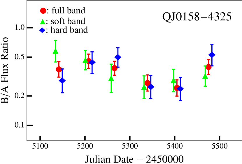
Figure 14: Chromatic X-ray microlensing light curves for QJ 0158$-$4325 in the full (0.4–8.0 keV, red circles), soft (0.4–1.3 keV, green triangles), and hard (1.3–8.0 keV, blue diamonds) X-ray bands. The observation dates for the soft and hard bands are slightly offset for clarity. Uncertainties are $1\,\sigma.$

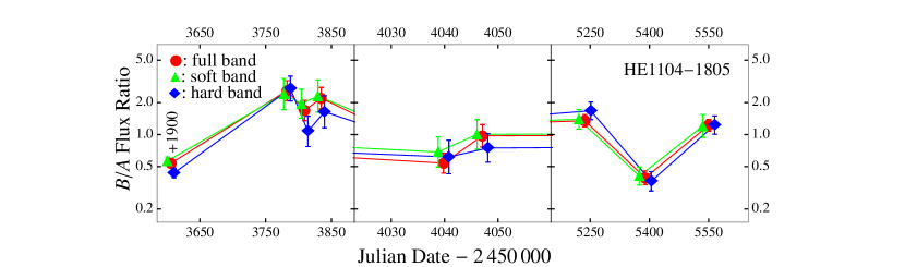
Figure 15: Chromatic X-ray microlensing light curves for HE 1104$-$1805 in the full (0.4–8.0 keV, red circles), soft (0.4–1.2 keV, green triangles), and hard (1.2–8.0 keV, blue diamonds) X-ray bands. Uncertainties are $1\,\sigma.$ The observation dates for the soft and hard bands are slightly offset for clarity. The first observation (made in 2000) was shifted by +1,900 days to better resolve other observations.

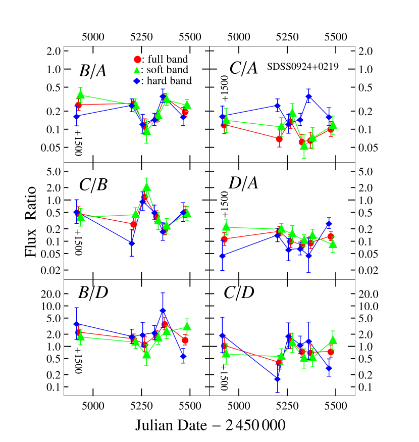
Figure 16: Chromatic X-ray microlensing light curves for SDSS 0924+0219 in the full (0.4–8.0 keV, red circles), soft (0.4–1.2 keV, green triangles), and hard (1.2–8 keV, blue diamonds) X-ray bands. The first observation (made in 2005) in each panel was shifted by +1,500 days in order to better resolve the next 5 observations (all made in 2010).

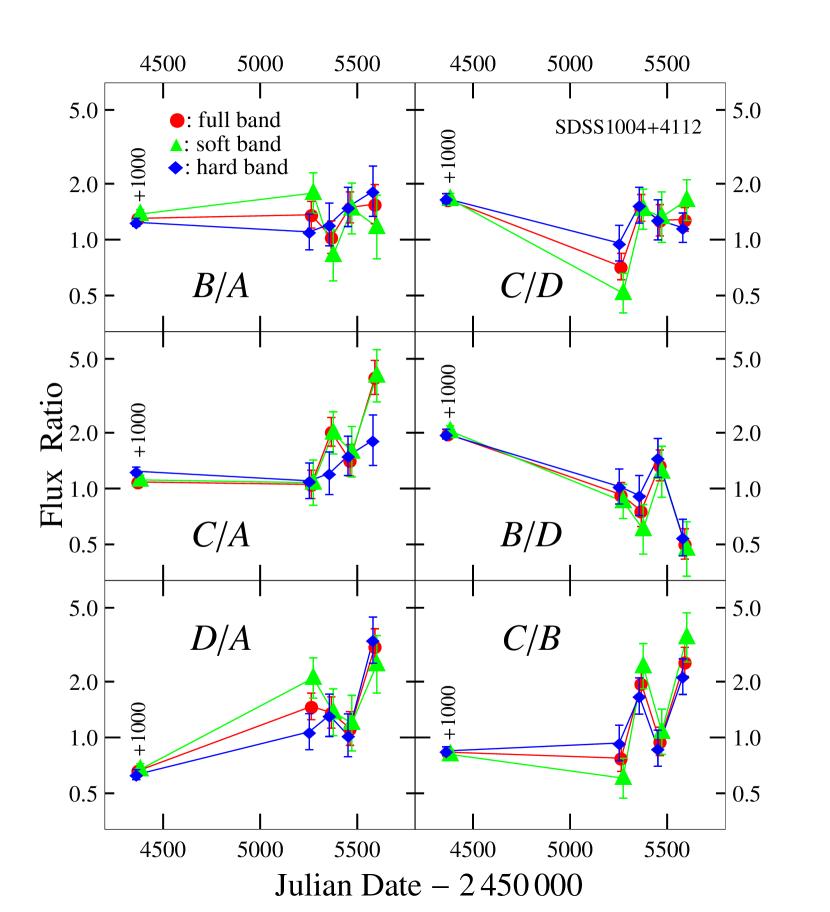
Figure 17: Chromatic X-ray microlensing light curves for SDSS 1004+4112 in the full (0.4–8.0 keV, red circles), soft (0.4–1.1 keV, green triangles), and hard (1.1–8 keV, blue diamonds) X-ray bands. The first observation (made in 2005) in each panel was shifted by +1,000 days in order to better resolve the next 4 observations (all made between 2010 and 2011).

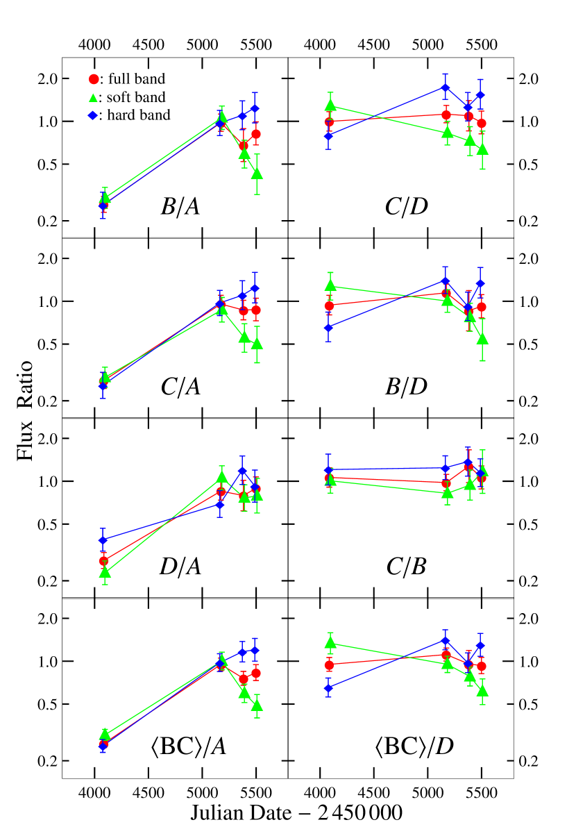
Figure 18: Chromatic X-ray microlensing light curves for HE 0435$-$1223 in the full (0.4–8.0 keV, red circles), soft (0.4–1.3 keV, green triangles), and hard (1.3–8 keV, blue diamonds) X-ray bands. In the last row, panels $\langle BC\rangle/A$ and $\langle BC\rangle/D$ show the light curves of the flux ratios between the intrinsic variability template (constructed from images B and C assuming their variability is intrinsic) and images A and D.

Our microlensing analysis is based on the image count rates presented in Tables 1–5. In principle, both microlensing by stars in the foreground galaxy and intrinsic variability of the background quasar can cause variability, and intrinsic variability modulated by time delays can mimic microlensing in any given eopch. In Q 2237+0305, the time delays are observationally constrained to be less than one day (Dai et al. 2003), and the intraday variability of the background quasar is measured to be only $\sim$1% of the total flux (Chartas et al. 2001; Dai et al. 2003). The time delays are longer in the other galaxy lenses, (less than 15 days in HE 0435–1223, Kochanek et al. 2006; Courbin et al. 2011; about 15 days in SDSS 0924+0219, Inada et al. 2003; $\leq 15$ days in QJ 0158–4325, Morgan et al. 2008; and $\sim$162 days in HE 1104$-$1805, Morgan et al. 2008). The effects of source variability will be most significant in the cluster lens SDSS 1004+4112, where the time delays between some of the images are several years (e.g., image C leads A by $\sim$822 days, image D lags A by lat least 1250 days, Fohlmeister et al. 2007, 2008). We focus on the evolution of the flux ratios between pairs of images to minimize the effects of intrinsic variability. If we were focused on flux ratios at a single epoch, the time delay is the relevant time scale over which we need to consider the effects of intrinsic variability. This would be a major problem for SDSS 1004+4112 with its long A/B to C or D delays. However, when we focus on microlensing through the time variability of flux ratios, we can prove mathematically that the relevant time scale for being affected by intrinsic variability is the shorter of the time delays and the sampling time scale. Hence for images C and D of SDSS 1004+4112, we need only worry about the intrinsic variability on times scales of order 90 days rather than the multi-year A/B to C/D time delays. Figures 14–18 show the evolution of the full, soft, and hard band flux ratios for QJ 0158$-$4325, HE 1104$-$1805, SDSS 0924+0219, SDSS 1004+4112, and HE 0435$-$1223, respectively. In these figures, we slightly offset the observation dates for the soft and hard bands for clarity. We have already discussed Q 2237+0305 in Chen et al. (2011).

5.1 X-ray Microlensing

In each lens system, we first fit the microlensing light curves (flux ratios) in each of the three bands as constants to test for the existence of microlensing variability. For example, in the two-image lens QJ 0158–4325 (Figure 14), we obtain $\chi^{2}=9.7$ (dof=5) with a null hypothesis probability of $\rm NP=0.08$ in the full band, $\chi^{2}=6.4$ with an $\rm NP=0.27$ in the soft band, and $\chi^{2}=8.92$ with an $\rm NP=0.11$ in the hard band. Thus we weakly detect microlensing in the full X-ray band. For HE 1104$-$1805 (Figure 15), we obtain $\chi^{2}=81.4$ (dof=8) with $\rm NP=2.5\times 10^{-14}$ in the full band, $\chi^{2}=33.4$ with $\rm NP=0.00005$ in the soft band, and $\chi^{2}=44.9$ with $\rm NP=3.8\times 10^{-7}$ in the hard band. Therefore we detect microlensing with high confidence in all three bands for HE 1104$-$1805. In the four image lenses SDSS 0924+0219, SDSS 1004+4112, and HE 0435–1223, where we have to test the existence of microlensing signal from each flux ratio combination, we summarize the microlensing statistics in Tables 14–16. In SDSS 0924+0219 (Figure 16 and Table 14), among the 6 pairs of flux ratios, the $B/A$ pair (images A and B are relatively brighter) gives the best statistical evidence for microlensing with a full band probability of $99.91\%$. The second most significant pair, C/B, shows microlensing at $94\%$ confidence for the full band. We also detect microlensing in SDSS 1004+4112 with high confidence (Figure 17 and Table 15). For example, considering the B/D pair in the full band, we have a $\chi^{2}=144.8$ for ${\rm dof}=4$ with a null hypothesis probability $\rm NP=2.6\times 10^{-30},$ in the soft band, we have a $\chi^{2}=72.2$ with an $\rm NP=7.7\times 10^{-15}$, and in the hard band, a $\chi^{2}=73.1$ with an $\rm NP=5.0\times 10^{-15}.$

The microlensing statistics of HE 0435$-$1223 are given in Table 16. We observe from Figure 18 that the flux ratios between images C and B are consistent with a constant, with $\chi^{2}=0.7,$ 0.96 and 0.31 (dof =3) for a model with no variability in the full, soft, and hard bands. This suggests that the variability of images B and C is mostly intrinsic during the observations reported in this paper. This can also be seen from the similarity between the light curve of B/A and that of C/A, or from the similarity between the light curves C/D and B/D (Figure 18). From Figure 18 and Table 16, we see that there is strong evidence for microlensing in image A of HE 0435$-$1223. For example, when fitting B/A ratio as a constant (dof=3), we obtain a $\chi^{2}=40.8$ with an $\rm NP=7.3\times 10^{-9}$ in the full band, a $\chi^{2}=17.3$ with an $\rm NP=0.0006$ in the soft band, and a $\chi^{2}=29.8$ and an $\rm NP=1.5\times 10^{-6}$ in the hard band. As for image D, when fitting the light curves of B/D or C/D pair with constants, we find that the light curve is roughly consistent with constant in the full band; however, this is not true when fitting the soft or hard band light curves. For example, from the B/D light curve, the full band fit gives $\chi^{2}=1.4$ (dof=3) with a one sided probability of 0.30, whereas the soft band fit gives a $\chi^{2}=6.0$ with an $\rm NP=0.11$ and the hard band fits gives a $\chi^{2}=6.9$ and an NP value 0.07. This suggests that image D of HE 0435$-$1223 is also gravitationally microlensed and that the lensing is energy-dependent with changes in the soft band opposite from those in the hard band (see next section). We assume that the variability of images B and C is intrinsic and use their noise-weighted mean, $\langle BC\rangle$, as an estimate of the intrinsic variability. We show the flux ratio $\langle BC\rangle$/A between image A and $\langle BC\rangle$ (the intrinsic variability template), and between image D and $\langle BC\rangle$, $\langle BC\rangle$/D, in Figure 18. When we fit $\langle BC\rangle$/A as a constant, we obtain $\chi^{2}=101.4$ with an NP value of $7.9\times 10^{-22}$ in the full band, $\chi^{2}=33.4$ and an $\rm NP=2.7\times 10^{-7}$ in the soft band, and $\chi^{2}=63.0$ and an $\rm NP=1.4\times 10^{-13}$ in the hard band. We therefore detect microlensing in image A with high confidence. This interpretation is confirmed by the better sampled optical light curves presented in Blackburne et al. (2012). Fitting the light curve $\langle BC\rangle$/D with a constant, we obtain a $\chi^{2}=1.5$ with a one sided probability of 0.32 in the full band, a $\chi^{2}=9.1$ with an $NP=0.03$ in the soft band, and a $\chi^{2}=14.1$ with an $NP=0.003$ in the hard band. Therefore, we detect microlensing in image D of HE 0435–1223.

5.2 X-ray Energy-Dependent Microlensing

Next, we test for differences between the soft and the hard energy bands, although only the observations of Q 2237+0305 were designed to have enough counts for this purpose. For the two-image lenses QJ 0158–4325 and HE 1104–1805, we can simplify compute the $\chi^{2}$ between the soft and hard band flux ratios. In QJ 0158–4325, we find $\chi^{2}=6.8$ (dof=6) with a null hypothesis probability $\rm NP=0.35$, which suggests no significant chromatic microlensing. Among the six observations of QJ 0158$-$4325 (Figure 14), epochs No. 1, 3, and 6 show differences in flux ratios between the soft and hard bands, whereas the other three epochs do not. In HE 1104$-$1805, we find $\chi^{2}=7.2$ (dof=9) which also suggests no significant chromatic microlensing.

For the four-image lenses SDSS 0924+0219, SDSS 1004+4112, and HE 0435–1223, we construct a $\chi^{2}$ test for energy-dependent microlensing using

$$\chi^{2}=\sum_{i,j}{\left[\frac{(d^{\rm hard}_{ij}-s^{\rm hard}_{i}-\mu^{\rm hard}_{j}-\delta_{ij})^{2}}{(\sigma^{\rm hard}_{ij})^{2}}+\frac{(d^{\rm soft}_{ij}-s^{\rm soft}_{i}-\mu^{\rm soft}_{j}-\delta_{ij})^{2}}{(\sigma^{\rm soft}_{ij})^{2}}\right]},$$ (1)

where $d^{\rm soft}_{ij}$ and $d^{\rm hard}_{ij}$ are the observed count rates in the soft and hard bands at epoch $i$ in image $j,$ $s^{\rm soft}_{i}$ and $s^{\rm hard}_{i}$ are the separate source light curves in the soft and hard bands at epoch $i,$ $\mu^{\rm soft}_{j}$ and $\mu^{\rm hard}_{j}$ are the mean magnification of the soft and hard bands in image $j,$ and $\delta_{ij}$ is the microlensing variability at epoch $i$ in image $j$ assumed to be the same for the soft and the hard bands. If there is an energy dependence (i.e., $\delta^{\rm soft}_{ij}\neq\delta^{\rm hard}_{ij}$), a model with $\delta_{ij}=\delta^{\rm soft}_{ij}=\delta^{\rm hard}_{ij}$ should fit poorly. For SDSS 1004+4112, we obtain $\chi^{2}=13.4$ (dof=5) with null hypothesis probability $\rm NP=0.02.$ For SDSS 0924+0219, we obtain $\chi^{2}=18.6$ (dof=7) with $\rm NP=0.009.$ For HE 0435–1223, we find $\chi^{2}=21.6$ (dof=3) with $\rm NP=0.00008.$ Therefore, we detect energy-dependent microlensing at $98\%,$ $99.1\%$ and $99.99\%$ confidence for these three four-image lenses.

Although we have detected Fe K$\alpha$ lines, which probably originate from a different region from the hard X-ray continuum and contaminate the microlensing light curves, the typical equivalent widths of the line are only 0.2–0.3 keV (observed frame) and do not contribute significantly to the hard band X-ray flux. This means that the differential microlensing between the soft and hard X-ray bands cannot be attributed to the presence of the iron lines. For example, if we use hard band microlensing light curves excluding the spectral segment containing the Fe K$\alpha$ emission (2.0–2.5 keV observed frame), we find that the Chen et al. (2011) results for Q 2237+0305 are unchanged.

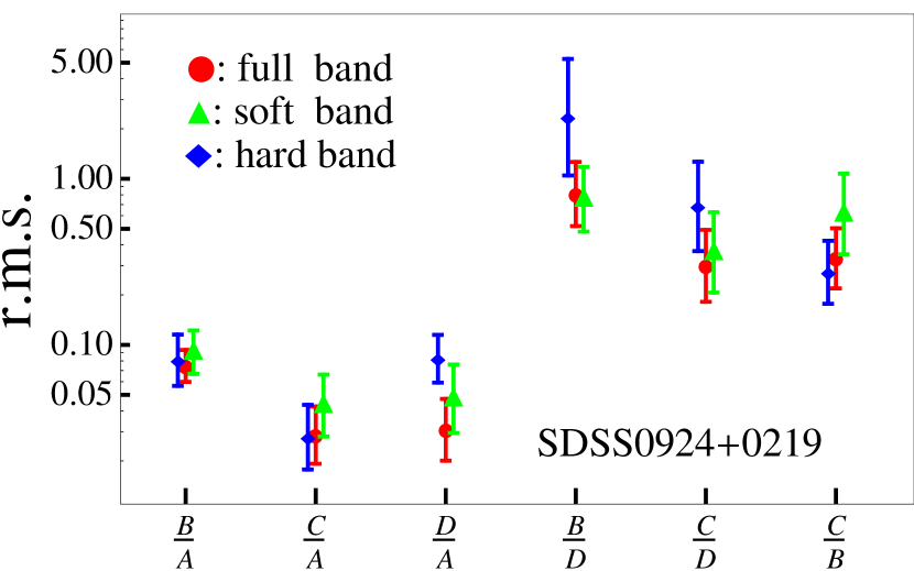
Figure 19: X-ray microlensing variability amplitudes of SDSS 0924+0219 in the full, soft and hard X-ray bands.

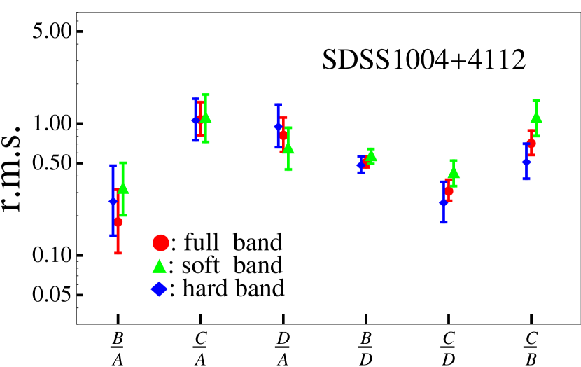
Figure 20: X-ray microlensing variability amplitudes of SDSS 1004+4112 in the full, soft and hard X-ray bands.

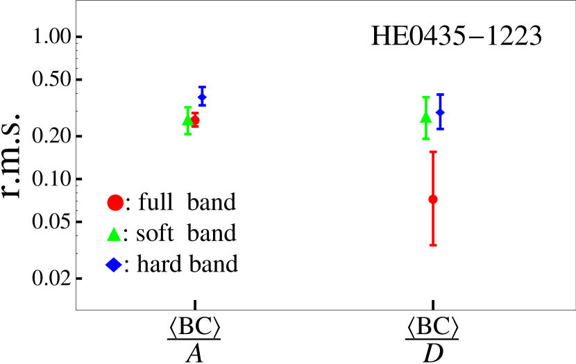
Figure 21: X-ray microlensing variability amplitudes of HE 0435$-$1223 in the full, soft and hard X-ray bands. Here “$\langle BC\rangle$” indicates the intrinsic variability template constructed from images B and C.

Unfortunately, this statistical detection of an energy dependence is difficult to visualize. For example, in Figures 19–21 we show the RMS flux ratios for various image combinations in SDSS 0924+0219, SDSS 1004+4112, and HE 0435–1223. Except for Q 2237+0305 (Chen et al. 2011) and image A of HE 0435$-$1223, any energy dependence is not visually obvious. Recall, however, that these observations are limited to integration times shorter than those needed to measure the hard/soft band light curves well.

5.3 Microlensing of the Fe K$\alpha$ Line

Microlensing of the Fe K$\alpha$ line has previously been detected in MG J0414+0534 (Chartas et al. 2002), Q 2237+0305 (Dai et al. 2003), H 1413+117 (Chartas et al. 2007), and SDSS 1004+4112 (Ota et al. 2006). For the six lenses with Fe K$\alpha$ detections in the combined spectra (Table 13 and Figure 13), we can test for microlensing by searching for changes in the line (EW or profile) between the images. Unfortunately we can only use the combined spectra rather than examining individual epochs because the S/N of the individual epochs is too low. This time averaging will smooth and reduce any microlensing signal.

In principle, if the continuum is microlensed differently from the lines, the equivalent widths (EWs) of the lines of the different images will differ. The effect tends to be one-sided even though microlensing can both magnify or demagnify a source. The demagnified regions tend to be smooth and wide, and thus demagnify large and small regions almost equally, while magnified regions have the caustics that will more strongly magnify compact emission regions. Thus there will be a tendency for lensed quasars to have either larger or smaller EWs than unlensed quasars depending on whether the line emitting region is smaller or larger then the continuum. We fit the EWs of the images as constants in each lens system (except SDSS 0924+0219, see Figure 12). For QJ 0158$-$4325, HE 1104$-$1805, SDSS 1004+4112, and HE 0435$-$1223, the EWs of the images are well fit by constants of 0.57 keV, 0.38 keV, 0.60 keV, and 0.88 keV, respectively, whereas the EW of image C of Q 2237+0305 differs from those of the other images. For Q 2237+0305, we obtain a best fit constant EW of 0.50 keV with $\chi^{2}=4.87$ (dof = 3) and an NP value of $0.18$, which weakly suggests differential microlensing effects between the X-ray continua and the Fe K$\alpha$ line. Overall, we conclude that the flux ratios of the Fe K$\alpha$ lines are comparable to those of the X-ray continua. Of course this null result does not mean that the Fe K$\alpha$ line is not microlensed, rather it implies that the size of the Fe K$\alpha$ emission has to be comparable to the X-ray continuum emitting region.

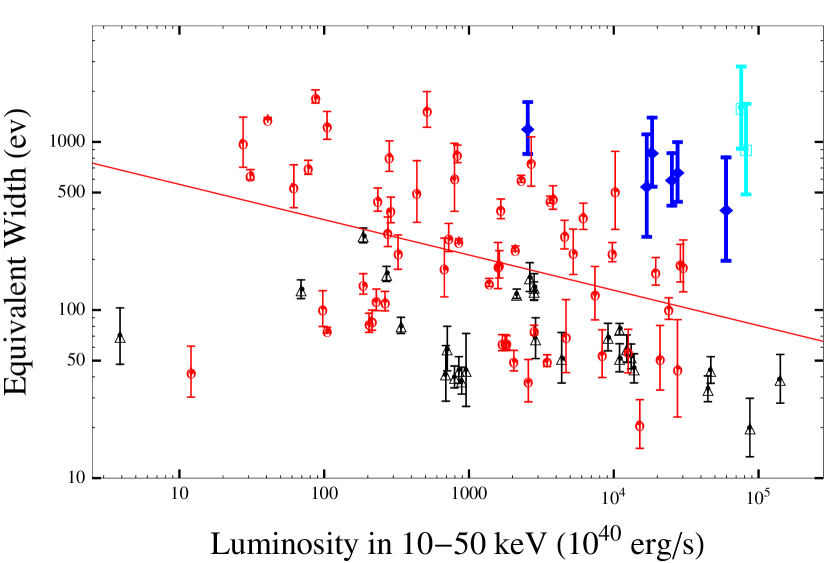
Figure 22: Equivalent width of Fe K$\alpha$  lines as a function of rest frame X-ray luminosity (10–50 keV) for SDSS 0924+0219, QJ 0158$-$4325, HE 0435$-$1223, Q 2237+0305, SDSS 1004+4112, and HE 1104$-$1805 (left to right, blue diamonds). H 1413+117 (Chartas et al. 2007) and MG J0414+0534 (Chartas et al. 2002) are marked by cyan squares. The black triangles (red circles) are AGN with absorption column densities greater (less) than $10^{22}\>\rm cm^{-2}$ (Fukazawa et al. 2011). The red line is the best fit to the low absorption systems (red points) as a power-law with additional intrinsic scatter in the $\rm EWs.$

As another test, we compared the EW–Luminosity relation of these six lenses (Table 17) with those of 88 nearby Seyfert galaxies observed by Suzaku (Fukazawa et al. 2011). The inverse correlation between the EW of the iron line and the X-ray luminosity is referred to as the X-ray Baldwin effect, and was first discovered by Iwasawa & Taniguchi (1993) for neutral Fe K$\alpha$ lines and X-ray luminosities in the 2–10 keV band. Recently, Fukazawa et al. (2011) extended the trend to the 10–50 keV band and for ionized Fe K$\alpha$ lines. If the iron line emission region is smaller than the continuum and therefore more strongly microlensed, lenses should on average have higher EWs than unlensed quasars with similar luminosities. Figure 22 shows the results where we have divided the local samples into low ($<10^{22}\,\rm cm^{-2}$, red circles) and high ($>10^{22}\,\rm cm^{-2}$, black triangles) absorption systems. Our six points are marked by blue diamonds, where we have corrected for typical gravitational lensing magnifications of 16 for the four image lenses and 8 for the two image lenses. We also include the results for MG J0414+0534 (Chartas et al. 2002) and H 1413+117 (Chartas et al. 2007). The data from Fukazawa et al. (2011) clearly shows the X-ray Baldwin effect of declining EW with luminosity. The gravitationally lensed quasars have systematically higher EWs than typical AGN of similar X-ray luminosity (in the 10–50 keV band). To test if our data is statistically consistent with typical AGN, we first fit the data in Fukazawa et al. (2011) with a power-law model plus intrinsic scatter in equivalent widths, and obtain

$$\log{\rm EW}=(6.81\pm 0.51)-(0.21\pm 0.07)\log{\rm L}\pm(1.02\pm 0.11)$$ (2)

with a reduced $\chi^{2}=0.94.$ Compared to this relation and its scatter, the 8 lenses have a $\chi^{2}=25.2$ (dof = 8), which is inconsistent with the distribution of typical AGN even without considering that all eight lenses lie on one side of the relation. The difference cannot be resolved by errors in the magnification correction applied to the luminosity. These are uncertain by at most a factor of 2, while a change by a factor of 30 would be needed to explain the differences. This suggests that the Fe K$\alpha$ line is microlensed more strongly than the X-ray continua, which in turn implies that the Fe K$\alpha$  emission region is smaller than the X-ray continuum, confirming earlier conclusions (Dai et al. 2003; Popovi$\rm\acute{c}$ et al. 2003, 2006).

6 Discussion

In this paper, we report our Chandra monitoring observations of six gravitationally lensed quasars: QJ 0158$-$4325, HE 1104$-$1805, HE 0435$-$1223, SDSS 0924+0219, SDSS 1004+4112, and Q 2237+0305. We find that simple power-law models plus Gaussian emission lines modified by absorption provide good fits to the spectra. We do not detect the predicted reflection component, other than the metal emission lines, due to the low S/N in the hard X-ray band. We detect intrinsic spectral variability in two epochs for Q 2237+0305, and differential absorption between images in QJ 0158$-$4325, SDSS 1004+4112, HE 0435$-$1223, and Q 2237+0305, but not in HE 1104$-$1805, or SDSS 0924+0219. From the stacked spectra of each lens, we detect Fe K$\alpha$ lines in all lenses and in almost all images. In Q 2237+0305, we marginally detect the Ni XXVII K$\alpha$ line in images A and D.

We clearly detect X-ray microlensing in all six lenses, and this can now be analyzed to determine the size of the X-ray emitting regions. The first of these analyses, for HE 0435$-$1223, is presented in Blackburne et al. (2012). Of these 6 lenses, the integration times were designed to provide accurate measurements in multiple bands only for Q 2237+0305. For this lens, we clearly see energy-dependent microlensing. Despite the lower S/N of the observations of the remaining 5 lenses, we still succeed in detecting energy-dependent microlensing in HE 0435$-$1223, SDSS 1004+4112, and SDSS 0924+0219, but not QJ 0158$-$4325 or HE 1104$-$1805.

In general, we do not see shifts in the Fe K$\alpha$ energy or EW between images for these lenses, except for Q 2237+0305 and HE 0435$-$1223, which implies that the sizes of the iron line emission regions are comparable to those of the X-ray continua. However, since the Fe K$\alpha$ line is extracted from the time averaged spectrum of each image, any microlensing effect has been smoothed. We note, however, that the lenses seem to have significantly higher EWs than a sample of 88 nearby Seyfert galaxies observed by Suzaku (Fukazawa et al. 2011). This suggests that the Fe K$\alpha$ line is more strongly microlensed than the X-ray continuum, and this implies a smaller emission region for the iron lines. This comparison is made at fixed luminosity, so it is not simply due to comparing local Seyferts with higher redshift more luminous quasars. Since the size of the X-ray continuum is already constrained to be small, $\sim$$10\,r_{g}$ (Morgan et al. 2008; Chartas et al. 2009; Dai et al. 2010; Blackburne et al. 2012), the Fe K$\alpha$ emission must come from the very inner region of the disk. The existence of chromatic microlensing between the soft and hard X-ray bands and the constraints on the size of the line emission region have important implications for testing general relativity in the strong field regime and the theoretical modeling of quasar accretion disks.

Although X-ray emission is one of the defining characteristic of AGN, the origin of this emission is still unknown. Unlike X-ray binaries, the AGN accretion disk itself is not hot enough to generate X-rays. The X-ray emission is generally attributed to inverse Compton scattering of soft UV photons from the accretion disk by hot electrons from a “corona” (see review of Reynolds & Nowak 2003). Although the origin of the hot electrons in the corona is debated, recent microlensing analyses have constrained the extent of this corona to be of order $10~{}r_{g}$ (Morgan et al. 2008; Chartas et al. 2009; Dai et al. 2010; Blackburne et al. 2012). Combining the results of this paper and Chen et al. (2011), we further find that the corona might have a temperature gradient with higher temperature electrons occupying a smaller volume.

Several models have been proposed to heat the electrons. In the classic “sandwich” corona model (Haardt & Maraschi 1991, 1993) and its extension, the “patchy” corona model (Haardt et al. 1994), the gravitational energy of the accretion disk is assumed to be transferred into the disk and corona with constant fractions. This group of models is in conflict with the microlensing results, since they predict similar sizes for the X-ray and optical emission regions, whereas the microlensing studies uniformly find smaller X-ray emission sizes than optical sizes (Pooley et al. 2006; Morgan et al. 2008; Chartas et al. 2009; Dai et al. 2010; Blackburne et al. 2011; Blackburne et al. 2012). However, simply requiring that the energy transfer process operates only on scales $\lesssim 10~{}r_{g}$ will solve this problem. A second group of models assumes that the X-ray emission is composed of a large number of flares triggered by magnetic field re-connections (e.g., Collin et al. 2003; Czerny et al. 2004; Torricelli-Ciamponi et al. 2005; Trzesniewski et al. 2011). The flare models can be considered as realistic realizations of the “patchy” corona model, and have advantages for interpreting the X-ray variability of AGN. Another difference from the steady corona models is that the electron distribution is mostly non-thermal in the flare models (Torricelli-Ciamponi et al. 2005). In general, the flare models predict similar X-ray and optical emission sizes for the microlensing analysis, because the corona is composed of a larger number of flares and the flares are randomly distributed over the disk. Some recent developments of the flare model specify that an avalanche of flares will be triggered by a single flare with a preferred direction of the triggered flares to the black hole (Trzesniewski et al. 2011), which will result in a smaller X-ray emission size at the disk center. A final set of models heat electrons with shocks. For example, Ghisellini et al. (2004) proposed the aborted jet model, where a jet launched near the black hole cannot escape the potential well, returns, and collides with other material to form shocks. These shocks then convert the kinetic energy of the aborted jet into thermal energy. This model predicts compact X-ray emission regions, possibly consistent with the microlensing results.

Given a disk-corona geometry, there should also be a reflection component created by the X-ray irradiation of the disk. Complicated radiative transfer processes occur during the reflection and the resulting continuum emission peaks at $\sim 50$ keV and produces metal emission lines, such as Fe K$\alpha$ (e.g., George & Fabian 1991). Based on the geometry of the model, one would expect the reflection region to be much larger than the corona, because the reflection can occur anywhere in the disk, a disk wind, or a surrounding torus. With the discovery of broad, skewed Fe K$\alpha$ lines in many Seyferts (e.g., MCG6–30–15, Tanaka et al. 1995), the reflection component near the black hole must contribute significantly to the total emissivity. In addition, the reflection components in some Seyferts are measured to be constant while the X-ray continuum is variable. Fabian & Vaughan (2003) proposed a light bending model, where the majority of the X-ray emission will illuminate the accretion disk due to the light bending effect by the black hole, producing the constant reflection component, and the escaping X-ray photons produce the X-ray continuum. If the X-ray source moves vertically above the accretion disk, it will produce a variable X-ray continuum and almost constant reflection component. In a competing model, Miller et al. (2008) proposed that the reflection occurs in the disk wind and that the redshifted Fe K$\alpha$ lines are artifacts created by a forest of warm absorbers in the X-ray bands. Our microlensing results suggest that the Fe K$\alpha$ emission region is compact and comparable in size or smaller than the X-ray continuum region, which prefers the light bending model over the disk-wind model.

We have composed, for the first time, a modest sample of quasar microlensing light curves in the full, soft, and hard X-ray bands, and a sample of Fe K$\alpha$ measurements in lensed quasars. Microlensing of the X-ray emission of lensed quasar is now clearly established in the full band (Morgan et al. 2001; Dai et al. 2003; Blackburne et al. 2006; Morgan et al. 2008; Chartas et al. 2009; Dai et al. 2010; Chen et al. 2011; Blackburne et al. 2011, 2012), and in the Fe K$\alpha$ lines (Chartas et al. 2002, 2004; Dai et al. 2003; Popovi$\rm\acute{c}$ et al. 2003, 2006). There are well-defined methods of analyzing the results to estimate the sizes of the X-ray emission regions (Kochanek 2004; Kochanek et al. 2007; Dai et al. 2010; Blackburne et al. 2012). To date, these analyses have yielded only upper bounds on the sizes of the X-ray emission regions because of the sparse X-ray light curves and most observations are too short to study multiple energy bands or the Fe K$\alpha$ emission in detail. There are, however, no observational or theoretical limits to obtaining the necessary data as long as the Chandra observatory continues to operate. Unfortunately, this science will become impossible with Chandra’s demise because no future mission is designed to have the necessary angular resolution.

We acknowledge the support from the NASA/SAO grants GO0-11121A/B/C/D, GO1-12139A/B/C, and GO2-13132A/B/C. CSK and JAB are supported by NSF grant AST-1009756. CWM is grateful for support by the National Science Foundation under Grant No. AST-0907848.

Table 1: Absorption-Corrected Count Rates for QJ 0158$-$4325.

ObsId	11556	11557	11558	11559	11560	11561
Date	2009-11-06	2010-01-12	2010-03-10	2010-05-23	2010-07-28	2010-10-06
Exposure (s)	5026	5016	5035	4942	4946	4944
${\rm A_{full}}$	$28.4{\pm 2.9}$	$33.6{\pm 3.3}$	$34.4{\pm 3.0}$	$35.9{\pm 3.3}$	$37.3{\pm 3.5}$	$30.7{\pm 2.9}$
${\rm A_{soft}}$	$13.3{\pm 2.1}$	$18.3{\pm 2.4}$	$20.5{\pm 3.5}$	$20.1{\pm 2.5}$	$18.6{\pm 2.5}$	$20.3{\pm 2.4}$
${\rm A_{hard}}$	$13.5{\pm 1.8}$	$14.7{\pm 2.2}$	$13.5{\pm 1.8}$	$15.8{\pm 2.0}$	$17.4{\pm 2.0}$	$10.4{\pm 1.5}$
${\rm B_{full}}$	$10.7{\pm 1.6}$	$15.2{\pm 2.1}$	$13.3{\pm 1.8}$	$9.7{\pm 1.6}$	$9.0{\pm 1.5}$	$12.2{\pm 1.8}$
${\rm B_{soft}}$	$7.7{\pm 1.5}$	$8.5{\pm 1.6}$	$6.2{\pm 1.8}$	$5.0{\pm 1.2}$	$5.4{\pm 1.2}$	$6.5{\pm 1.3}$
${\rm B_{hard}}$	$3.9{\pm 1.0}$	$6.5{\pm 1.3}$	$6.7{\pm 1.3}$	$3.9{\pm 1.0}$	$4.1{\pm 1.0}$	$5.4{\pm 1.1}$
${\rm bkg_{full}}$	$2.97$	$1.92$	$3.13$	$4.97$	$3.37$	$2.66$
${\rm bkg_{soft}}$	$0.35$	$0.35$	$0.35$	$0.89$	$0.18$	$0.35$
${\rm bkg_{hard}}$	$2.62$	$1.57$	$2.79$	$4.08$	$3.19$	$2.30$

Table 2: Absorption-Corrected Count Rates for HE 1104$-$1805.

ObsId	375	6918	6917	6919	6920	6921	11553	11554	11555
Date	2000-06-10	2006-02-16	2006-03-15	2006-04-09	2006-10-31	2006-11-08	2010-02-09	2010-07-12	2010-12-20
Exposure (s)	47425	4959	4549	4865	5007	4915	12756	12758	12757
${\rm A_{full}}$	$25.3{\pm 0.8}$	$8.4{\pm 1.5}$	$10.3{\pm 1.7}$	$7.5{\pm 1.4}$	$16.2{\pm 2.2}$	$13.4{\pm 2.3}$	$10.8{\pm 1.1}$	$23.5{\pm 2.1}$	$11.7{\pm 1.1}$
${\rm A_{soft}}$	$15.1{\pm 0.8}$	$3.9{\pm 1.0}$	$5.3{\pm 1.3}$	$3.8{\pm 1.1}$	$9.0{\pm 1.9}$	$7.3{\pm 1.6}$	$5.6{\pm 0.9}$	$11.2{\pm 1.2}$	$5.3{\pm 1.0}$
${\rm A_{hard}}$	$10.3{\pm 0.7}$	$4.2{\pm 0.9}$	$5.4{\pm 1.2}$	$4.0{\pm 1.1}$	$5.9{\pm 1.4}$	$6.4{\pm 1.3}$	$4.2{\pm 0.6}$	$11.5{\pm 1.4}$	$5.9{\pm 0.8}$
${\rm B_{full}}$	$13.6{\pm 0.6}$	$21.8{\pm 2.8}$	$17.3{\pm 2.5}$	$16.5{\pm 2.3}$	$8.7{\pm 1.5}$	$13.0{\pm 2.3}$	$14.5{\pm 1.3}$	$9.3{\pm 1.1}$	$14.3{\pm 1.2}$
${\rm B_{soft}}$	$8.6{\pm 0.6}$	$9.3{\pm 1.8}$	$10.4{\pm 2.0}$	$8.9{\pm 1.8}$	$6.1{\pm 1.5}$	$7.3{\pm 1.7}$	$7.7{\pm 1.1}$	$4.6{\pm 0.7}$	$6.4{\pm 1.1}$
${\rm B_{hard}}$	$4.5{\pm 0.4}$	$11.3{\pm 1.7}$	$5.8{\pm 1.4}$	$6.5{\pm 1.4}$	$3.6{\pm 1.0}$	$4.8{\pm 1.1}$	$7.0{\pm 0.9}$	$4.2{\pm 0.7}$	$7.2{\pm 1.0}$
${\rm bkg_{full}}$	$3.14$	$1.99$	$2.65$	$8.11$	$3.94$	$2.68$	$2.06$	$3.18$	$3.01$
${\rm bkg_{soft}}$	$1.02$	$0.22$	$0.72$	$1.80$	$0.88$	$0.45$	$0.09$	$0.43$	$0.94$
${\rm bkg_{hard}}$	$2.13$	$1.77$	$1.93$	$6.31$	$3.06$	$2.23$	$1.98$	$2.75$	$2.06$

Table 3: Absorption-Corrected Count Rates for SDSS 0924+0219.

ObsId	5604	11562	11563	11564	11565	11566
Date	2005-02-24	2010-01-13	2010-03-10	2010-05-10	2010-06-22	2010-10-05
Exposure (s)	17944	21542	21264	21642	21546	21543
${\rm A_{full}}$	$6.6{\pm 0.8}$	$12.0{\pm 1.3}$	$8.0{\pm 0.8}$	$18.5{\pm 1.2}$	$13.6{\pm 1.2}$	$9.9{\pm 0.8}$
${\rm A_{soft}}$	$3.6{\pm 0.6}$	$7.0{\pm 1.0}$	$3.9{\pm 0.6}$	$9.8{\pm 0.9}$	$7.2{\pm 0.9}$	$5.8{\pm 0.6}$
${\rm A_{hard}}$	$2.6{\pm 0.4}$	$4.8{\pm 0.6}$	$3.7{\pm 0.5}$	$7.8{\pm 0.7}$	$5.9{\pm 0.9}$	$3.5{\pm 0.5}$
${\rm B_{full}}$	$1.7{\pm 0.3}$	$3.2{\pm 0.5}$	$0.9{\pm 0.2}$	$2.8{\pm 0.4}$	$4.6{\pm 0.5}$	$1.9{\pm 0.3}$
${\rm B_{soft}}$	$1.3{\pm 0.3}$	$1.7{\pm 0.4}$	$0.4{\pm 0.1}$	$1.6{\pm 0.3}$	$2.2{\pm 0.4}$	$1.4{\pm 0.3}$
${\rm B_{hard}}$	$0.4{\pm 0.1}$	$1.2{\pm 0.3}$	$0.4{\pm 0.1}$	$1.1{\pm 0.2}$	$2.1{\pm 0.5}$	$0.6{\pm 0.2}$
${\rm C_{full}}$	$0.8{\pm 0.3}$	$0.8{\pm 0.3}$	$1.1{\pm 0.3}$	$1.2{\pm 0.3}$	$0.9{\pm 0.3}$	$1.0{\pm 0.3}$
${\rm C_{soft}}$	$0.5{\pm 0.2}$	$0.8{\pm 0.3}$	$0.7{\pm 0.2}$	$0.5{\pm 0.2}$	$0.5{\pm 0.2}$	$0.7{\pm 0.2}$
${\rm C_{hard}}$	$0.2{\pm 0.1}$	$0.1{\pm 0.1}$	$0.4{\pm 0.2}$	$0.6{\pm 0.2}$	$0.4{\pm 0.2}$	$0.3{\pm 0.1}$
${\rm D_{full}}$	$0.7{\pm 0.3}$	$2.1{\pm 0.5}$	$0.8{\pm 0.3}$	$1.5{\pm 0.3}$	$1.3{\pm 0.4}$	$1.3{\pm 0.3}$
${\rm D_{soft}}$	$0.8{\pm 0.3}$	$1.4{\pm 0.4}$	$0.6{\pm 0.3}$	$1.0{\pm 0.3}$	$1.0{\pm 0.3}$	$0.5{\pm 0.2}$
${\rm D_{hard}}$	$0.1{\pm 0.1}$	$0.7{\pm 0.2}$	$0.2{\pm 0.1}$	$0.5{\pm 0.2}$	$0.3{\pm 0.3}$	$1.0{\pm 0.3}$
${\rm bkg_{full}}$	$1.41$	$2.53$	$2.57$	$2.70$	$2.98$	$2.35$
${\rm bkg_{soft}}$	$0.22$	$0.27$	$0.27$	$0.72$	$0.81$	$0.63$
${\rm bkg_{hard}}$	$1.19$	$2.26$	$2.29$	$1.98$	$2.17$	$1.72$

Table 4: Absorption-Corrected Count Rates for SDSS 1004+4112.

ObsId	5794	11546	11547	11548	11549
Date	2005-01-01	2010-03-08	2010-06-19	2010-09-23	2011-01-30
Exposure (s)	79987	5957	5960	5963	5959
${\rm A_{full}}$	$17.4{\pm 0.5}$	$12.2{\pm 1.5}$	$9.1{\pm 1.3}$	$8.5{\pm 1.3}$	$5.4{\pm 1.0}$
${\rm A_{soft}}$	$8.1{\pm 0.3}$	$4.8{\pm 1.0}$	$4.3{\pm 0.9}$	$3.2{\pm 0.8}$	$2.3{\pm 0.7}$
${\rm A_{hard}}$	$9.2{\pm 0.4}$	$7.2{\pm 1.2}$	$4.7{\pm 0.9}$	$5.2{\pm 1.0}$	$3.0{\pm 0.8}$
${\rm B_{full}}$	$22.7{\pm 0.6}$	$16.6{\pm 1.8}$	$9.4{\pm 1.3}$	$12.7{\pm 1.5}$	$8.4{\pm 1.3}$
${\rm B_{soft}}$	$11.1{\pm 0.4}$	$8.5{\pm 1.3}$	$3.5{\pm 0.8}$	$4.8{\pm 1.0}$	$2.7{\pm 0.7}$
${\rm B_{hard}}$	$11.4{\pm 0.4}$	$7.9{\pm 1.2}$	$5.7{\pm 1.0}$	$7.7{\pm 1.2}$	$5.5{\pm 1.0}$
${\rm C_{full}}$	$18.9{\pm 0.5}$	$12.8{\pm 1.6}$	$18.4{\pm 1.9}$	$12.1{\pm 1.5}$	$21.5{\pm 2.0}$
${\rm C_{soft}}$	$9.0{\pm 0.4}$	$5.1{\pm 1.0}$	$8.6{\pm 1.3}$	$5.1{\pm 1.0}$	$9.3{\pm 1.4}$
${\rm C_{hard}}$	$9.6{\pm 0.4}$	$7.4{\pm 1.2}$	$9.5{\pm 1.3}$	$6.8{\pm 1.1}$	$11.8{\pm 1.5}$
${\rm D_{full}}$	$11.5{\pm 0.4}$	$17.9{\pm 1.9}$	$12.4{\pm 1.6}$	$9.6{\pm 1.4}$	$16.7{\pm 1.9}$
${\rm D_{soft}}$	$5.4{\pm 0.3}$	$10.0{\pm 1.5}$	$5.9{\pm 1.2}$	$3.9{\pm 0.9}$	$5.7{\pm 1.2}$
${\rm D_{hard}}$	$5.8{\pm 0.3}$	$7.7{\pm 1.2}$	$6.2{\pm 1.1}$	$5.3{\pm 1.0}$	$10.1{\pm 1.4}$

Table 5: Absorption-Corrected Count Rates for HE 0435$-$1223.

ObsId	7761	11550	11551	11552
Date	2006-12-17	2009-12-07	2010-07-04	2010-10-29
Exposure (s)	9994	12876	12757	12758
${\rm A_{full}}$	$41.5{\pm 2.7}$	$12.9{\pm 1.3}$	$12.1{\pm 1.4}$	$7.6{\pm 1.0}$
${\rm A_{soft}}$	$25.8{\pm 2.3}$	$7.3{\pm 1.0}$	$7.3{\pm 1.1}$	$4.5{\pm 0.8}$
${\rm A_{hard}}$	$13.3{\pm 1.4}$	$4.7{\pm 0.7}$	$3.6{\pm 0.6}$	$2.9{\pm 0.5}$
${\rm B_{full}}$	$10.8{\pm 1.2}$	$12.6{\pm 1.2}$	$8.3{\pm 2.0}$	$6.3{\pm 0.8}$
${\rm B_{soft}}$	$7.5{\pm 1.1}$	$7.7{\pm 1.0}$	$4.3{\pm 0.7}$	$1.9{\pm 0.5}$
${\rm B_{hard}}$	$3.4{\pm 0.6}$	$4.6{\pm 0.7}$	$4.0{\pm 0.7}$	$3.6{\pm 0.6}$
${\rm C_{full}}$	$11.5{\pm 1.3}$	$12.3{\pm 1.2}$	$10.5{\pm 1.2}$	$6.7{\pm 0.9}$
${\rm C_{soft}}$	$7.5{\pm 1.1}$	$6.4{\pm 0.9}$	$4.0{\pm 0.7}$	$2.2{\pm 0.5}$
${\rm C_{hard}}$	$4.1{\pm 0.7}$	$5.7{\pm 0.7}$	$5.5{\pm 0.9}$	$4.1{\pm 0.6}$
${\rm D_{full}}$	$11.5{\pm 1.3}$	$11.0{\pm 1.1}$	$9.6{\pm 2.1}$	$6.8{\pm 0.9}$
${\rm D_{soft}}$	$5.9{\pm 1.0}$	$7.7{\pm 1.0}$	$5.6{\pm 0.8}$	$3.5{\pm 0.7}$
${\rm D_{hard}}$	$5.2{\pm 0.8}$	$3.3{\pm 0.5}$	$4.3{\pm 0.7}$	$2.7{\pm 0.5}$
${\rm bkg_{full}}$	$1.48$	$2.43$	$3.03$	$2.38$
${\rm bkg_{soft}}$	$0.41$	$0.83$	$0.71$	$0.64$
${\rm bkg_{hard}}$	$1.07$	$1.60$	$2.32$	$1.74$

Table 6: Absorption-Corrected Count Rates for Q 2237+0305.

No.	ObsId	HJD	Exposure	$\rm{A_{full}}$	$\rm{A_{soft}}$	$\rm{A_{hard}}$	$\rm{B_{full}}$	$\rm{B_{soft}}$	$\rm{B_{hard}}$	$\rm{C_{full}}$	$\rm{C_{soft}}$	$\rm{C_{hard}}$	$\rm{D_{full}}$	$\rm{D_{soft}}$	$\rm{D_{hard}}$	$\rm{b_{full}}$	$\rm{b_{soft}}$	$\rm{b_{hard}}$
I	431	51794	30287	$70.2{\pm 2.3}$	$49.2{\pm 2.0}$	$21.5{\pm 1.0}$	$16.0{\pm 1.1}$	$10.9{\pm 1.0}$	$4.7{\pm 0.5}$	$34.1{\pm 1.6}$	$26.3{\pm 1.5}$	$8.8{\pm 0.6}$	$17.1{\pm 1.3}$	$13.5{\pm 1.4}$	$4.2{\pm 0.5}$	$2.8$	$0.7$	$2.1$
II	1632	52252	9535	$59.7{\pm 4.5}$	$38.5{\pm 4.4}$	$19.0{\pm 1.8}$	$11.1{\pm 1.4}$	$8.9{\pm 1.5}$	$3.0{\pm 0.6}$	$19.1{\pm 1.9}$	$11.3{\pm 1.9}$	$7.0{\pm 1.0}$	$13.7{\pm 1.8}$	$11.8{\pm 1.9}$	$3.4{\pm 0.7}$	$2.0$	$0.7$	$1.3$
III	6831	53745	7264	$23.9{\pm 2.5}$	$14.6{\pm 2.1}$	$8.6{\pm 1.2}$	$22.9{\pm 2.5}$	$11.5{\pm 2.1}$	$8.9{\pm 1.3}$	$6.7{\pm 1.3}$	$3.2{\pm 1.0}$	$2.8{\pm 0.7}$	$14.0{\pm 2.2}$	$11.3{\pm 2.4}$	$3.5{\pm 0.9}$	$2.3$	$0.9$	$1.4$
IV	6832	53856	7936	$46.2{\pm 3.4}$	$27.6{\pm 3.0}$	$18.2{\pm 1.7}$	$27.6{\pm 2.7}$	$15.7{\pm 2.3}$	$9.8{\pm 1.3}$	$23.1{\pm 2.5}$	$14.0{\pm 2.0}$	$6.9{\pm 1.1}$	$21.0{\pm 2.6}$	$13.4{\pm 2.4}$	$6.2{\pm 1.1}$	$3.2$	$1.1$	$2.1$
V	6833	53882	7953	$30.3{\pm 2.7}$	$16.4{\pm 2.3}$	$11.4{\pm 1.6}$	$12.1{\pm 1.7}$	$7.6{\pm 1.6}$	$4.1{\pm 0.8}$	$11.2{\pm 1.6}$	$6.2{\pm 1.3}$	$4.3{\pm 0.8}$	$6.7{\pm 1.4}$	$4.5{\pm 1.4}$	$2.1{\pm 0.6}$	$2.3$	$0.4$	$1.9$
VI	6834	53912	7938	$64.7{\pm 4.1}$	$38.6{\pm 3.5}$	$23.4{\pm 1.9}$	$27.5{\pm 2.6}$	$19.6{\pm 2.5}$	$8.1{\pm 1.1}$	$17.5{\pm 2.0}$	$9.6{\pm 1.7}$	$6.3{\pm 1.0}$	$17.4{\pm 2.3}$	$10.0{\pm 2.1}$	$5.9{\pm 1.0}$	$3.6$	$1.2$	$2.3$
VII	6835	53938	7871	$73.8{\pm 4.7}$	$30.2{\pm 3.2}$	$33.0{\pm 2.3}$	$20.0{\pm 2.2}$	$14.0{\pm 2.2}$	$6.1{\pm 1.0}$	$13.9{\pm 1.8}$	$9.6{\pm 1.8}$	$4.5{\pm 0.8}$	$16.2{\pm 2.2}$	$10.3{\pm 2.2}$	$5.3{\pm 0.9}$	$2.8$	$0.7$	$2.1$
VIII	6836	53964	7928	$43.9{\pm 3.4}$	$24.4{\pm 2.7}$	$15.4{\pm 1.7}$	$13.2{\pm 1.8}$	$6.7{\pm 1.5}$	$5.7{\pm 0.9}$	$11.8{\pm 1.6}$	$5.2{\pm 1.2}$	$5.0{\pm 0.9}$	$10.8{\pm 1.7}$	$5.5{\pm 1.5}$	$4.8{\pm 0.9}$	$2.5$	$0.7$	$1.8$
IX	6837	53994	7944	$37.9{\pm 3.3}$	$21.0{\pm 2.7}$	$14.9{\pm 1.5}$	$18.5{\pm 2.1}$	$10.7{\pm 1.9}$	$6.4{\pm 1.0}$	$9.8{\pm 1.5}$	$5.2{\pm 1.3}$	$3.4{\pm 0.7}$	$11.9{\pm 1.9}$	$8.7{\pm 2.0}$	$3.5{\pm 0.8}$	$3.0$	$0.7$	$2.3$
X	6838	54017	7984	$36.1{\pm 3.4}$	$24.6{\pm 2.9}$	$9.8{\pm 1.2}$	$12.8{\pm 1.8}$	$8.7{\pm 1.7}$	$4.6{\pm 0.9}$	$11.7{\pm 1.6}$	$5.9{\pm 1.4}$	$4.7{\pm 0.9}$	$9.8{\pm 1.6}$	$4.0{\pm 1.3}$	$4.7{\pm 0.9}$	$3.2$	$0.3$	$2.9$
XI	6839	54069	7873	$133.4{\pm 5.8}$	$76.0{\pm 4.9}$	$49.7{\pm 2.9}$	$52.1{\pm 3.6}$	$31.3{\pm 3.2}$	$18.0{\pm 1.8}$	$30.8{\pm 2.8}$	$18.5{\pm 2.4}$	$10.8{\pm 1.3}$	$39.1{\pm 3.5}$	$29.4{\pm 3.6}$	$10.6{\pm 1.5}$	$4.7$	$1.1$	$3.6$
XII	6840	54115	7976	$94.5{\pm 4.8}$	$71.1{\pm 5.3}$	$30.7{\pm 2.3}$	$37.6{\pm 3.3}$	$26.1{\pm 3.1}$	$10.2{\pm 1.3}$	$32.7{\pm 3.0}$	$22.1{\pm 2.6}$	$8.1{\pm 1.1}$	$36.8{\pm 3.7}$	$23.9{\pm 3.5}$	$10.0{\pm 1.4}$	$3.3$	$0.7$	$2.6$
XIII	11534	55197	28454	$116.5{\pm 2.9}$	$68.9{\pm 2.5}$	$42.1{\pm 1.4}$	$35.8{\pm 1.6}$	$22.0{\pm 1.4}$	$12.2{\pm 0.7}$	$11.0{\pm 0.9}$	$6.4{\pm 0.7}$	$3.8{\pm 0.4}$	$76.9{\pm 2.5}$	$53.9{\pm 2.6}$	$22.9{\pm 1.1}$	$4.4$	$1.5$	$2.9$
XIV	11535	55312	29432	$21.3{\pm 1.2}$	$9.7{\pm 0.9}$	$9.9{\pm 1.0}$	$6.9{\pm 0.7}$	$3.5{\pm 0.5}$	$2.6{\pm 0.3}$	$3.2{\pm 0.5}$	$1.0{\pm 0.3}$	$1.5{\pm 0.2}$	$13.0{\pm 1.0}$	$5.5{\pm 0.8}$	$4.8{\pm 0.7}$	$3.1$	$0.7$	$2.4$
XV	11536	55374	27891	$23.0{\pm 1.3}$	$9.3{\pm 0.9}$	$10.6{\pm 0.7}$	$7.3{\pm 0.7}$	$3.6{\pm 0.6}$	$2.9{\pm 0.4}$	$2.8{\pm 0.4}$	$1.1{\pm 0.3}$	$1.2{\pm 0.2}$	$15.3{\pm 1.2}$	$7.0{\pm 1.0}$	$6.0{\pm 0.5}$	$2.6$	$0.7$	$2.0$
XVI	11537	55416	29355	$14.7{\pm 1.0}$	$6.5{\pm 0.8}$	$5.8{\pm 0.5}$	$4.4{\pm 0.5}$	$1.9{\pm 0.4}$	$2.0{\pm 0.3}$	$2.9{\pm 0.4}$	$0.7{\pm 0.2}$	$1.5{\pm 0.3}$	$9.4{\pm 0.9}$	$3.8{\pm 0.7}$	$4.5{\pm 0.5}$	$3.3$	$0.9$	$2.4$
XVII	11538	55471	29354	$34.0{\pm 1.5}$	$15.3{\pm 1.2}$	$14.7{\pm 0.8}$	$10.3{\pm 0.8}$	$5.2{\pm 0.7}$	$4.1{\pm 0.4}$	$3.3{\pm 0.5}$	$1.8{\pm 0.4}$	$1.2{\pm 0.2}$	$34.3{\pm 1.7}$	$20.7{\pm 1.6}$	$11.7{\pm 0.7}$	$2.7$	$0.8$	$1.9$
XVIII	11539	55524	9828	$17.6{\pm 2.0}$	$6.0{\pm 1.2}$	$9.6{\pm 1.1}$	$6.4{\pm 1.2}$	$1.1{\pm 0.5}$	$3.3{\pm 0.7}$	$2.8{\pm 0.8}$	$1.0{\pm 0.5}$	$1.1{\pm 0.4}$	$10.0{\pm 1.6}$	$5.8{\pm 1.4}$	$2.9{\pm 0.6}$	$2.9$	$0.7$	$2.2$
XIX	13195	55526	9830	$16.3{\pm 1.9}$	$6.7{\pm 1.4}$	$7.5{\pm 1.0}$	$5.3{\pm 1.0}$	$1.6{\pm 0.7}$	$2.6{\pm 0.6}$	$2.1{\pm 0.7}$	$1.0{\pm 0.5}$	$0.8{\pm 0.4}$	$8.3{\pm 1.4}$	$3.4{\pm 1.2}$	$3.4{\pm 0.7}$	$3.5$	$0.8$	$2.7$
XX	13191	55528	9828	$15.7{\pm 1.8}$	$5.7{\pm 1.3}$	$7.6{\pm 1.0}$	$4.4{\pm 1.0}$	$1.8{\pm 0.7}$	$1.9{\pm 0.5}$	$2.0{\pm 0.6}$	$1.1{\pm 0.5}$	$0.7{\pm 0.3}$	$7.2{\pm 1.3}$	$3.0{\pm 1.1}$	$2.9{\pm 0.6}$	$2.2$	$0.7$	$1.6$

Table 7: Fits to the Chandra  spectra of QJ 0158$-$4325.

Fit	Epoch	Image	$\Gamma$	$\rm{N_{H}}$	Flux	Flux	$\chi^{2}_{\nu}(\nu)$	$P(\chi^{2}/{\nu})$
				$\times 10^{22}$	$\times 10^{-13}$	$\times 10^{-13}$
				$\rm{cm^{-2}}$	$\rm{erg~{}s^{-1}~{}cm^{-2}}$	$\rm{erg~{}s^{-1}~{}cm^{-2}}$
$1$	I	A	$1.86^{+0.17}_{-0.17}$	$0.10^{+0.19}_{-0.10}$	$0.37^{+0.04}_{-0.09}$	$1.02^{+0.20}_{-0.22}$	$1.24(16)$	$0.23$
$1$	I	B	$\cdot$	$0.00^{+0.05}_{-0.00}$	$0.16^{+0.01}_{-0.06}$	$0.33^{+0.10}_{-0.10}$	$\cdot$	$\cdot$
$2$	II	A	$1.95^{+0.23}_{-0.21}$	$0.00^{+0.04}_{-0.00}$	$0.48^{+0.08}_{-0.07}$	$0.87^{+0.20}_{-0.17}$	$1.27(20)$	$0.19$
$2$	II	B	$\cdot$	$0.04^{+0.08}_{-0.04}$	$0.27^{+0.03}_{-0.05}$	$0.54^{+0.13}_{-0.12}$	$\cdot$	$\cdot$
$3$	III	A	$2.00^{+0.15}_{-0.15}$	$0.02^{+0.13}_{-0.02}$	$0.58^{+0.02}_{-0.15}$	$1.05^{+0.19}_{-0.21}$	$0.82(19)$	$0.68$
$3$	III	B	$\cdot$	$0.03^{+0.09}_{-0.03}$	$0.20^{+0.03}_{-0.05}$	$0.36^{+0.10}_{-0.09}$	$\cdot$	$\cdot$
$4$	IV	A	$1.79^{+0.17}_{-0.17}$	$0.00^{+0.06}_{-0.00}$	$0.51^{+0.07}_{-0.07}$	$1.17^{+0.23}_{-0.19}$	$1.30(19)$	$0.17$
$4$	IV	B	$\cdot$	$0.00^{+0.09}_{-0.00}$	$0.17^{+0.03}_{-0.03}$	$0.38^{+0.11}_{-0.09}$	$\cdot$	$\cdot$
$5$	V	A	$1.75^{+0.17}_{-0.16}$	$0.00^{+0.05}_{-0.00}$	$0.51^{+0.07}_{-0.07}$	$1.24^{+0.25}_{-0.21}$	$1.09(19)$	$0.35$
$5$	V	B	$\cdot$	$0.03^{+0.21}_{-0.03}$	$0.17^{+0.02}_{-0.04}$	$0.45^{+0.12}_{-0.11}$	$\cdot$	$\cdot$
$6$	VI	A	$2.06^{+0.19}_{-0.18}$	$0.02^{+0.10}_{-0.02}$	$0.56^{+0.03}_{-0.16}$	$0.92^{+0.26}_{-0.24}$	$1.28(18)$	$0.19$
$6$	VI	B	$\cdot$	$0.01^{+0.09}_{-0.01}$	$0.21^{+0.03}_{-0.06}$	$0.33^{+0.13}_{-0.10}$	$\cdot$	$\cdot$
$7$	stacked	A	$1.93^{+0.06}_{-0.06}$	$0.00^{+0.01}_{-0.00}$	$0.53^{+0.03}_{-0.03}$	$0.99^{+0.07}_{-0.07}$	$1.11(128)$	$0.18$
$7$	stacked	B	$\cdot$	$0.03^{+0.03}_{-0.02}$	$0.19^{+0.01}_{-0.01}$	$0.39^{+0.03}_{-0.03}$	$\cdot$	$\cdot$
$8$	stacked	A+B	$1.90^{+0.06}_{-0.06}$	$0.00^{+0.01}_{-0.00}$	$0.85^{+0.04}_{-0.04}$	$1.72^{+0.10}_{-0.10}$	$0.93(129)$	$0.70$

Table 8: Fits to the Chandra  spectra of HE 1104$-$1805.

Fit	Epoch	Image	$\Gamma$	$\rm{N_{H}}$	Flux	Flux	$\chi^{2}_{\nu}(\nu)$	$P(\chi^{2}/{\nu})$
				$\times 10^{22}$	$\times 10^{-13}$	$\times 10^{-13}$
				$\rm{cm^{-2}}$	$\rm{erg~{}s^{-1}~{}cm^{-2}}$	$\rm{erg~{}s^{-1}~{}cm^{-2}}$
$1$	I	A	$1.82^{+0.05}_{-0.05}$	$0.00^{+0.01}_{-0.00}$	$0.34^{+0.00}_{-0.03}$	$0.77^{+0.05}_{-0.05}$	$0.97(172)$	$0.59$
$1$	I	B	$\cdot$	$0.00^{+0.01}_{-0.00}$	$0.18^{+0.00}_{-0.01}$	$0.41^{+0.03}_{-0.03}$	$\cdot$	$\cdot$
$2$	II	A	$1.69^{+0.33}_{-0.26}$	$0.28^{+1.61}_{-0.28}$	$0.16^{+0.02}_{-0.05}$	$0.45^{+0.15}_{-0.18}$	$0.60(11)$	$0.83$
$2$	II	B	$\cdot$	$0.08^{+0.22}_{-0.08}$	$0.37^{+0.03}_{-0.06}$	$1.03^{+0.22}_{-0.22}$	$\cdot$	$\cdot$
$3$	III	A	$2.60^{+0.69}_{-0.53}$	$1.23^{+1.67}_{-1.23}$	$0.51^{+0.06}_{-0.05}$	$0.37^{+0.13}_{-0.16}$	$1.55(7)$	$0.15$
$3$	III	B	$\cdot$	$0.13^{+0.25}_{-0.13}$	$0.45^{+0.04}_{-0.08}$	$0.32^{+0.15}_{-0.11}$	$\cdot$	$\cdot$
$4$	IV	A	$2.11^{+0.41}_{-0.27}$	$1.00^{+1.28}_{-1.00}$	$0.29^{+0.03}_{-0.03}$	$0.42^{+0.16}_{-0.18}$	$0.65(6)$	$0.69$
$4$	IV	B	$\cdot$	$0.00^{+0.14}_{-0.00}$	$0.30^{+0.00}_{-0.09}$	$0.44^{+0.17}_{-0.13}$	$\cdot$	$\cdot$
$5$	V	A	$2.28^{+0.75}_{-0.33}$	$0.28^{+0.71}_{-0.28}$	$0.39^{+0.03}_{-0.08}$	$0.44^{+0.12}_{-0.16}$	$1.41(8)$	$0.19$
$5$	V	B	$\cdot$	$0.00^{+0.27}_{-0.00}$	$0.21^{+0.00}_{-0.08}$	$0.24^{+0.12}_{-0.09}$	$\cdot$	$\cdot$
$6$	VI	A	$1.82^{+0.34}_{-0.24}$	$0.00^{+0.67}_{-0.00}$	$0.22^{+0.01}_{-0.12}$	$0.49^{+0.15}_{-0.18}$	$1.13(8)$	$0.34$
$6$	VI	B	$\cdot$	$0.00^{+0.19}_{-0.00}$	$0.21^{+0.00}_{-0.07}$	$0.48^{+0.13}_{-0.14}$	$\cdot$	$\cdot$
$7$	VII	A	$1.88^{+0.20}_{-0.13}$	$0.03^{+0.28}_{-0.03}$	$0.20^{+0.01}_{-0.04}$	$0.42^{+0.06}_{-0.07}$	$0.59(30)$	$0.96$
$7$	VII	B	$\cdot$	$0.01^{+0.09}_{-0.01}$	$0.27^{+0.02}_{-0.04}$	$0.55^{+0.09}_{-0.08}$	$\cdot$	$\cdot$
$8$	VIII	A	$1.75^{+0.14}_{-0.11}$	$0.00^{+0.14}_{-0.00}$	$0.40^{+0.01}_{-0.10}$	$1.00^{+0.12}_{-0.14}$	$0.73(38)$	$0.89$
$8$	VIII	B	$\cdot$	$0.00^{+0.07}_{-0.00}$	$0.16^{+0.00}_{-0.04}$	$0.41^{+0.07}_{-0.07}$	$\cdot$	$\cdot$
$9$	VIIII	A	$1.74^{+0.14}_{-0.13}$	$0.00^{+0.13}_{-0.00}$	$0.17^{+0.00}_{-0.06}$	$0.44^{+0.07}_{-0.08}$	$1.10(32)$	$0.32$
$9$	VIIII	B	$\cdot$	$0.00^{+0.05}_{-0.00}$	$0.25^{+0.00}_{-0.05}$	$0.64^{+0.10}_{-0.10}$	$\cdot$	$\cdot$
$10$	II	A+B	$1.94^{+0.32}_{-0.28}$	$0.38^{+0.31}_{-0.26}$	$0.72^{+0.05}_{-0.06}$	$1.36^{+0.23}_{-0.26}$	$0.56(14)$	$0.90$
$11$	III	A+B	$2.36^{+0.44}_{-0.23}$	$0.00^{+0.40}_{-0.00}$	$0.68^{+0.06}_{-0.33}$	$0.69^{+0.13}_{-0.21}$	$1.05(10)$	$0.40$
$12$	IV	A+B	$1.99^{+0.29}_{-0.26}$	$0.00^{+0.18}_{-0.00}$	$0.45^{+0.03}_{-0.21}$	$0.79^{+0.20}_{-0.25}$	$1.15(9)$	$0.32$
$13$	V	A+B	$2.03^{+0.36}_{-0.25}$	$0.00^{+0.20}_{-0.00}$	$0.50^{+0.03}_{-0.19}$	$0.82^{+0.19}_{-0.22}$	$1.14(12)$	$0.32$
$14$	VI	A+B	$1.86^{+0.29}_{-0.26}$	$0.00^{+0.09}_{-0.00}$	$0.47^{+0.03}_{-0.21}$	$1.00^{+0.23}_{-0.28}$	$1.16(11)$	$0.31$
$15$	stacked	A	$1.81^{+0.03}_{-0.03}$	$0.00^{+0.01}_{-0.00}$	$0.31^{+0.00}_{-0.03}$	$0.71^{+0.03}_{-0.03}$	$1.40(48)$	$0.03$
$15$	stacked	B	$\cdot$	$0.00^{+0.01}_{-0.00}$	$0.23^{+0.00}_{-0.01}$	$0.52^{+0.03}_{-0.03}$	$\cdot$	$\cdot$
$16$	stacked	A	$1.76^{+0.05}_{-0.05}$	$0.00^{+0.01}_{-0.00}$	$0.30^{+0.00}_{-0.03}$	$0.74^{+0.04}_{-0.04}$	$1.38(47)$	$0.04$
$16$	stacked	B	$1.86^{+0.05}_{-0.05}$	$0.00^{+0.02}_{-0.00}$	$0.23^{+0.00}_{-0.01}$	$0.49^{+0.03}_{-0.03}$	$\cdot$	$\cdot$
$17$	stacked	A+B	$1.81^{+0.03}_{-0.03}$	$0.00^{+0.01}_{-0.00}$	$0.54^{+0.00}_{-0.03}$	$1.24^{+0.05}_{-0.05}$	$1.01(147)$	$0.45$

Table 9: Fits to the Chandra  spectra of SDSS 0924+0219.

Fit	Epoch	Image	$\Gamma$	$\rm{N_{H}}$	Flux	Flux	$\chi^{2}_{\nu}(\nu)$	$P(\chi^{2}/{\nu})$
				$\times 10^{22}$	$\times 10^{-13}$	$\times 10^{-13}$
				$\rm{cm^{-2}}$	$\rm{erg~{}s^{-1}~{}cm^{-2}}$	$\rm{erg~{}s^{-1}~{}cm^{-2}}$
$1$	I	A+C+D	$2.57^{+0.52}_{-0.44}$	$0.13^{+0.20}_{-0.13}$	$0.12^{+0.01}_{-0.03}$	$0.16^{+0.05}_{-0.05}$	$1.23(11)$	$0.26$
$1$	I	B	$\cdot$	$0.00^{+0.09}_{-0.00}$	$0.02^{+0.00}_{-0.01}$	$0.02^{+0.01}_{-0.01}$	$\cdot$	$\cdot$
$2$	II	A+C+D	$2.39^{+0.25}_{-0.13}$	$0.00^{+0.09}_{-0.00}$	$0.26^{+0.03}_{-0.03}$	$0.31^{+0.04}_{-0.04}$	$0.67(30)$	$0.92$
$2$	II	B	$\cdot$	$0.00^{+0.08}_{-0.00}$	$0.05^{+0.01}_{-0.01}$	$0.06^{+0.01}_{-0.01}$	$\cdot$	$\cdot$
$3$	III	A+C+D	$2.23^{+0.42}_{-0.37}$	$0.13^{+0.20}_{-0.13}$	$0.13^{+0.01}_{-0.02}$	$0.28^{+0.06}_{-0.06}$	$1.09(17)$	$0.35$
$3$	III	B	$\cdot$	$0.39^{+0.85}_{-0.39}$	$0.01^{+0.00}_{-0.00}$	$0.04^{+0.02}_{-0.02}$	$\cdot$	$\cdot$
$4$	IV	A+C+D	$2.02^{+0.13}_{-0.11}$	$0.00^{+0.04}_{-0.00}$	$0.30^{+0.02}_{-0.02}$	$0.62^{+0.07}_{-0.07}$	$0.79(44)$	$0.84$
$4$	IV	B	$\cdot$	$0.00^{+0.05}_{-0.00}$	$0.05^{+0.01}_{-0.01}$	$0.10^{+0.02}_{-0.02}$	$\cdot$	$\cdot$
$5$	V	A+C+D	$2.18^{+0.15}_{-0.13}$	$0.00^{+0.04}_{-0.00}$	$0.23^{+0.02}_{-0.02}$	$0.38^{+0.05}_{-0.05}$	$0.89(34)$	$0.65$
$5$	V	B	$\cdot$	$0.03^{+0.11}_{-0.03}$	$0.06^{+0.01}_{-0.01}$	$0.10^{+0.02}_{-0.02}$	$\cdot$	$\cdot$
$6$	VI	A+C+D	$2.07^{+0.21}_{-0.14}$	$0.00^{+0.08}_{-0.00}$	$0.19^{+0.02}_{-0.02}$	$0.36^{+0.05}_{-0.05}$	$0.95(27)$	$0.53$
$6$	VI	B	$\cdot$	$0.00^{+0.05}_{-0.00}$	$0.03^{+0.01}_{-0.01}$	$0.06^{+0.01}_{-0.01}$	$\cdot$	$\cdot$
$7$	stacked	A+C+D	$2.12^{+0.07}_{-0.05}$	$0.00^{+0.03}_{-0.00}$	$0.21^{+0.01}_{-0.01}$	$0.35^{+0.02}_{-0.02}$	$0.90(161)$	$0.81$
$7$	stacked	B	$\cdot$	$0.02^{+0.03}_{-0.02}$	$0.04^{+0.00}_{-0.00}$	$0.06^{+0.01}_{-0.01}$	$\cdot$	$\cdot$
$8$	stacked	A+C+D	$2.23^{+0.07}_{-0.05}$	$0.00^{+0.04}_{-0.00}$	$0.21^{+0.00}_{-0.02}$	$0.36^{+0.02}_{-0.02}$	$0.91(125)$	$0.77$
$9$	stacked	B	$2.14^{+0.15}_{-0.14}$	$0.00^{+0.07}_{-0.00}$	$0.04^{+0.00}_{-0.01}$	$0.06^{+0.01}_{-0.01}$	$0.69(27)$	$0.89$
$10$	stacked	A+B+C+D	$2.19^{+0.09}_{-0.08}$	$0.02^{+0.03}_{-0.02}$	$0.27^{+0.01}_{-0.02}$	$0.49^{+0.03}_{-0.03}$	$0.95(166)$	$0.65$

Table 10: Fits to the the Chandra  spectra of SDSS 1004+4112.

Fit	Epoch	Image	$\Gamma$	$\rm{N_{H}}$	Flux	Flux	$\chi^{2}_{\nu}(\nu)$	$P(\chi^{2}/{\nu})$
				$\times 10^{22}$	$\times 10^{-13}$	$\times 10^{-13}$
				$\rm{cm^{-2}}$	$\rm{erg~{}s^{-1}~{}cm^{-2}}$	$\rm{erg~{}s^{-1}~{}cm^{-2}}$
$1$	I	A	$1.98^{+0.04}_{-0.04}$	$0.03^{+0.04}_{-0.03}$	$0.27^{+0.01}_{-0.01}$	$0.61^{+0.03}_{-0.03}$	$1.13(559)$	$0.02$
$1$	I	B	$\cdot$	$0.05^{+0.01}_{-0.01}$	$0.34^{+0.01}_{-0.01}$	$0.82^{+0.03}_{-0.03}$	$\cdot$	$\cdot$
$1$	I	C	$\cdot$	$0.10^{+0.02}_{-0.02}$	$0.27^{+0.01}_{-0.01}$	$0.70^{+0.03}_{-0.03}$	$\cdot$	$\cdot$
$1$	I	D	$\cdot$	$0.14^{+0.02}_{-0.03}$	$0.14^{+0.01}_{-0.01}$	$0.40^{+0.02}_{-0.02}$	$\cdot$	$\cdot$
$2$	II	A	$2.08^{+0.17}_{-0.17}$	$0.33^{+0.60}_{-0.33}$	$0.15^{+0.06}_{-0.06}$	$0.52^{+0.10}_{-0.12}$	$0.95(34)$	$0.54$
$2$	II	B	$\cdot$	$0.08^{+0.09}_{-0.06}$	$0.27^{+0.03}_{-0.04}$	$0.59^{+0.12}_{-0.11}$	$\cdot$	$\cdot$
$2$	II	C	$\cdot$	$0.00^{+0.03}_{-0.00}$	$0.24^{+0.01}_{-0.06}$	$0.44^{+0.09}_{-0.09}$	$\cdot$	$\cdot$
$2$	II	D	$\cdot$	$0.07^{+0.07}_{-0.06}$	$0.27^{+0.04}_{-0.04}$	$0.59^{+0.11}_{-0.10}$	$\cdot$	$\cdot$
$3$	III	A	$2.00^{+0.18}_{-0.15}$	$0.00^{+0.16}_{-0.00}$	$0.16^{+0.03}_{-0.03}$	$0.33^{+0.06}_{-0.06}$	$1.05(29)$	$0.40$
$3$	III	B	$\cdot$	$0.00^{+0.07}_{-0.00}$	$0.16^{+0.02}_{-0.03}$	$0.33^{+0.07}_{-0.06}$	$\cdot$	$\cdot$
$3$	III	C	$\cdot$	$0.01^{+0.06}_{-0.01}$	$0.31^{+0.04}_{-0.04}$	$0.66^{+0.11}_{-0.10}$	$\cdot$	$\cdot$
$3$	III	D	$\cdot$	$0.11^{+0.12}_{-0.08}$	$0.18^{+0.03}_{-0.03}$	$0.46^{+0.08}_{-0.07}$	$\cdot$	$\cdot$
$4$	IV	A	$1.74^{+0.18}_{-0.17}$	$0.59^{+1.03}_{-0.59}$	$0.07^{+0.05}_{-0.04}$	$0.56^{+0.17}_{-0.20}$	$0.98(24)$	$0.48$
$4$	IV	B	$\cdot$	$0.00^{+0.08}_{-0.00}$	$0.20^{+0.01}_{-0.05}$	$0.62^{+0.17}_{-0.14}$	$\cdot$	$\cdot$
$4$	IV	C	$\cdot$	$0.00^{+0.02}_{-0.00}$	$0.20^{+0.01}_{-0.06}$	$0.63^{+0.13}_{-0.13}$	$\cdot$	$\cdot$
$4$	IV	D	$\cdot$	$0.14^{+0.23}_{-0.13}$	$0.12^{+0.02}_{-0.03}$	$0.47^{+0.12}_{-0.11}$	$\cdot$	$\cdot$
$5$	V	A	$1.97^{+0.14}_{-0.15}$	$0.00^{+0.90}_{-0.00}$	$0.10^{+0.02}_{-0.02}$	$0.23^{+0.06}_{-0.05}$	$1.02(29)$	$0.43$
$5$	V	B	$\cdot$	$0.00^{+0.05}_{-0.00}$	$0.11^{+0.02}_{-0.02}$	$0.25^{+0.06}_{-0.05}$	$\cdot$	$\cdot$
$5$	V	C	$\cdot$	$0.00^{+0.02}_{-0.00}$	$0.37^{+0.04}_{-0.04}$	$0.82^{+0.13}_{-0.12}$	$\cdot$	$\cdot$
$5$	V	D	$\cdot$	$0.19^{+0.16}_{-0.10}$	$0.21^{+0.03}_{-0.03}$	$0.67^{+0.11}_{-0.10}$	$\cdot$	$\cdot$
$6$	stacked	A	$1.99^{+0.03}_{-0.03}$	$0.04^{+0.03}_{-0.03}$	$0.24^{+0.01}_{-0.01}$	$0.55^{+0.02}_{-0.02}$	$1.15(659)$	$0.01$
$6$	stacked	B	$\cdot$	$0.09^{+0.01}_{-0.01}$	$0.30^{+0.01}_{-0.01}$	$0.77^{+0.03}_{-0.03}$	$\cdot$	$\cdot$
$6$	stacked	C	$\cdot$	$0.09^{+0.01}_{-0.01}$	$0.27^{+0.01}_{-0.01}$	$0.69^{+0.02}_{-0.02}$	$\cdot$	$\cdot$
$6$	stacked	D	$\cdot$	$0.13^{+0.02}_{-0.02}$	$0.16^{+0.01}_{-0.01}$	$0.43^{+0.02}_{-0.02}$	$\cdot$	$\cdot$
$7$	stacked	A	$1.93^{+0.07}_{-0.05}$	$0.00^{+0.04}_{-0.00}$	$0.24^{+0.01}_{-0.01}$	$0.59^{+0.03}_{-0.03}$	$1.11(149)$	$0.17$
$8$	stacked	B	$1.98^{+0.05}_{-0.04}$	$0.00^{+0.02}_{-0.00}$	$0.33^{+0.01}_{-0.01}$	$0.75^{+0.03}_{-0.03}$	$0.84(180)$	$0.94$
$9$	stacked	C	$1.93^{+0.05}_{-0.04}$	$0.01^{+0.04}_{-0.01}$	$0.29^{+0.01}_{-0.01}$	$0.71^{+0.03}_{-0.03}$	$0.73(167)$	$1.00$
$10$	stacked	D	$1.87^{+0.10}_{-0.09}$	$0.06^{+0.06}_{-0.05}$	$0.16^{+0.01}_{-0.01}$	$0.47^{+0.03}_{-0.03}$	$0.89(116)$	$0.80$
$11$	stacked	A+B+C+D	$1.95^{+0.04}_{-0.04}$	$0.04^{+0.02}_{-0.02}$	$1.14^{+0.02}_{-0.02}$	$2.89^{+0.07}_{-0.07}$	$0.98(375)$	$0.61$

Table 11: Fits to the Chandra  spectra of HE 0435$-$1223.

Fit	Epoch	Image	$\Gamma$	$\rm{N_{H}}$	Flux	Flux	$\chi^{2}_{\nu}(\nu)$	$P(\chi^{2}/{\nu})$
				$\times 10^{22}$	$\times 10^{-13}$	$\times 10^{-13}$
				$\rm{cm^{-2}}$	$\rm{erg~{}s^{-1}~{}cm^{-2}}$	$\rm{erg~{}s^{-1}~{}cm^{-2}}$
$1$	I	A	$2.00^{+0.11}_{-0.10}$	$0.08^{+0.08}_{-0.08}$	$0.41^{+0.04}_{-0.03}$	$0.95^{+0.11}_{-0.10}$	$1.02(58)$	$0.43$
$1$	I	B	$\cdot$	$0.00^{+0.03}_{-0.00}$	$0.18^{+0.02}_{-0.02}$	$0.35^{+0.05}_{-0.05}$	$\cdot$	$\cdot$
$1$	I	C	$\cdot$	$0.00^{+0.03}_{-0.00}$	$0.17^{+0.02}_{-0.02}$	$0.34^{+0.05}_{-0.05}$	$\cdot$	$\cdot$
$1$	I	D	$\cdot$	$0.12^{+0.16}_{-0.10}$	$0.14^{+0.02}_{-0.02}$	$0.37^{+0.06}_{-0.05}$	$\cdot$	$\cdot$
$2$	II	A	$1.93^{+0.11}_{-0.10}$	$0.00^{+0.12}_{-0.00}$	$0.17^{+0.02}_{-0.02}$	$0.36^{+0.05}_{-0.05}$	$0.96(50)$	$0.56$
$2$	II	B	$\cdot$	$0.00^{+0.05}_{-0.00}$	$0.18^{+0.02}_{-0.02}$	$0.39^{+0.06}_{-0.05}$	$\cdot$	$\cdot$
$2$	II	C	$\cdot$	$0.00^{+0.05}_{-0.00}$	$0.16^{+0.02}_{-0.02}$	$0.36^{+0.06}_{-0.05}$	$\cdot$	$\cdot$
$2$	II	D	$\cdot$	$0.00^{+0.04}_{-0.00}$	$0.13^{+0.02}_{-0.02}$	$0.28^{+0.04}_{-0.04}$	$\cdot$	$\cdot$
$3$	III	A	$1.71^{+0.12}_{-0.11}$	$0.00^{+0.08}_{-0.00}$	$0.12^{+0.02}_{-0.02}$	$0.36^{+0.05}_{-0.05}$	$1.15(39)$	$0.24$
$3$	III	B	$\cdot$	$0.06^{+0.14}_{-0.06}$	$0.09^{+0.01}_{-0.01}$	$0.32^{+0.05}_{-0.05}$	$\cdot$	$\cdot$
$3$	III	C	$\cdot$	$0.00^{+0.11}_{-0.00}$	$0.12^{+0.02}_{-0.02}$	$0.37^{+0.06}_{-0.05}$	$\cdot$	$\cdot$
$3$	III	D	$\cdot$	$0.00^{+0.09}_{-0.00}$	$0.12^{+0.02}_{-0.01}$	$0.36^{+0.06}_{-0.05}$	$\cdot$	$\cdot$
$4$	IV	A	$1.58^{+0.27}_{-0.23}$	$0.00^{+0.23}_{-0.00}$	$0.09^{+0.02}_{-0.02}$	$0.33^{+0.06}_{-0.06}$	$1.35(23)$	$0.12$
$4$	IV	B	$\cdot$	$0.31^{+0.55}_{-0.29}$	$0.05^{+0.01}_{-0.01}$	$0.34^{+0.07}_{-0.06}$	$\cdot$	$\cdot$
$4$	IV	C	$\cdot$	$0.00^{+0.08}_{-0.00}$	$0.07^{+0.01}_{-0.01}$	$0.24^{+0.06}_{-0.05}$	$\cdot$	$\cdot$
$4$	IV	D	$\cdot$	$0.08^{+0.19}_{-0.08}$	$0.06^{+0.01}_{-0.01}$	$0.27^{+0.06}_{-0.05}$	$\cdot$	$\cdot$
$5$	stacked	A	$1.81^{+0.05}_{-0.05}$	$0.00^{+0.03}_{-0.00}$	$0.18^{+0.01}_{-0.01}$	$0.47^{+0.03}_{-0.03}$	$1.09(187)$	$0.20$
$5$	stacked	B	$\cdot$	$0.00^{+0.03}_{-0.00}$	$0.12^{+0.01}_{-0.01}$	$0.32^{+0.02}_{-0.02}$	$\cdot$	$\cdot$
$5$	stacked	C	$\cdot$	$0.00^{+0.03}_{-0.00}$	$0.13^{+0.01}_{-0.01}$	$0.33^{+0.02}_{-0.02}$	$\cdot$	$\cdot$
$5$	stacked	D	$\cdot$	$0.02^{+0.05}_{-0.02}$	$0.11^{+0.01}_{-0.01}$	$0.31^{+0.02}_{-0.02}$	$\cdot$	$\cdot$
$6$	stacked	A	$2.06^{+0.09}_{-0.09}$	$0.08^{+0.08}_{-0.07}$	$0.18^{+0.01}_{-0.02}$	$0.42^{+0.04}_{-0.04}$	$1.04(56)$	$0.39$
$7$	stacked	B	$1.87^{+0.13}_{-0.11}$	$0.00^{+0.05}_{-0.00}$	$0.13^{+0.01}_{-0.01}$	$0.32^{+0.02}_{-0.02}$	$1.12(35)$	$0.28$
$8$	stacked	C	$1.59^{+0.11}_{-0.10}$	$0.00^{+0.04}_{-0.00}$	$0.11^{+0.01}_{-0.01}$	$0.42^{+0.05}_{-0.04}$	$0.99(41)$	$0.49$
$9$	stacked	D	$1.89^{+0.11}_{-0.11}$	$0.07^{+0.12}_{-0.07}$	$0.11^{+0.01}_{-0.01}$	$0.30^{+0.04}_{-0.04}$	$0.94(37)$	$0.58$
$10$	stacked	A+B+C+D	$1.90^{+0.07}_{-0.07}$	$0.04^{+0.04}_{-0.03}$	$0.62^{+0.02}_{-0.03}$	$1.61^{+0.08}_{-0.08}$	$0.97(171)$	$0.61$

Table 12: Fits to the Chandra  spectra of Q 2237+0305.

Fit	Epoch	Image	$\Gamma$	$\rm{N_{H}}$	Flux	Flux	$\chi^{2}_{\nu}(\nu)$	$P(\chi^{2}/{\nu})$
				$\times 10^{22}$	$\times 10^{-13}$	$\times 10^{-13}$
				$\rm{cm^{-2}}$	$\rm{erg~{}s^{-1}~{}cm^{-2}}$	$\rm{erg~{}s^{-1}~{}cm^{-2}}$
$1$	I	A	$1.88^{+0.07}_{-0.07}$	$0.02^{+0.02}_{-0.02}$	$0.52^{+0.02}_{-0.02}$	$1.37^{+0.08}_{-0.08}$	$1.03(103)$	$0.39$
$1$	I	B	$\cdot$	$0.00^{+0.02}_{-0.00}$	$0.10^{+0.00}_{-0.02}$	$0.24^{+0.03}_{-0.03}$	$\cdot$	$\cdot$
$1$	I	C	$\cdot$	$0.05^{+0.02}_{-0.02}$	$0.20^{+0.01}_{-0.01}$	$0.57^{+0.05}_{-0.04}$	$\cdot$	$\cdot$
$1$	I	D	$\cdot$	$0.02^{+0.02}_{-0.02}$	$0.11^{+0.01}_{-0.01}$	$0.28^{+0.03}_{-0.03}$	$\cdot$	$\cdot$
$2$	II	A	$1.77^{+0.10}_{-0.10}$	$0.02^{+0.05}_{-0.02}$	$0.36^{+0.03}_{-0.03}$	$1.08^{+0.13}_{-0.12}$	$1.13(50)$	$0.25$
$2$	II	B	$\cdot$	$0.00^{+0.04}_{-0.00}$	$0.09^{+0.01}_{-0.01}$	$0.25^{+0.05}_{-0.05}$	$\cdot$	$\cdot$
$2$	II	C	$\cdot$	$0.08^{+0.08}_{-0.06}$	$0.12^{+0.02}_{-0.02}$	$0.45^{+0.07}_{-0.07}$	$\cdot$	$\cdot$
$2$	II	D	$\cdot$	$0.02^{+0.04}_{-0.02}$	$0.12^{+0.02}_{-0.02}$	$0.35^{+0.06}_{-0.06}$	$\cdot$	$\cdot$
$3$	III	A	$1.79^{+0.20}_{-0.21}$	$0.06^{+0.17}_{-0.06}$	$0.16^{+0.03}_{-0.03}$	$0.58^{+0.14}_{-0.12}$	$1.82(17)$	$0.02$
$3$	III	B	$\cdot$	$0.00^{+0.04}_{-0.00}$	$0.13^{+0.02}_{-0.02}$	$0.34^{+0.10}_{-0.08}$	$\cdot$	$\cdot$
$3$	III	C	$\cdot$	$0.00^{+0.10}_{-0.00}$	$0.05^{+0.01}_{-0.01}$	$0.14^{+0.05}_{-0.04}$	$\cdot$	$\cdot$
$3$	III	D	$\cdot$	$0.02^{+0.14}_{-0.02}$	$0.07^{+0.02}_{-0.01}$	$0.21^{+0.06}_{-0.05}$	$\cdot$	$\cdot$
$4$	IV	A	$1.90^{+0.22}_{-0.15}$	$0.05^{+0.10}_{-0.05}$	$0.37^{+0.03}_{-0.07}$	$1.07^{+0.15}_{-0.16}$	$0.91(48)$	$0.65$
$4$	IV	B	$\cdot$	$0.00^{+0.10}_{-0.00}$	$0.21^{+0.01}_{-0.05}$	$0.50^{+0.11}_{-0.10}$	$\cdot$	$\cdot$
$4$	IV	C	$\cdot$	$0.04^{+0.06}_{-0.04}$	$0.17^{+0.02}_{-0.03}$	$0.47^{+0.08}_{-0.09}$	$\cdot$	$\cdot$
$4$	IV	D	$\cdot$	$0.00^{+0.02}_{-0.00}$	$0.15^{+0.00}_{-0.05}$	$0.36^{+0.08}_{-0.08}$	$\cdot$	$\cdot$
$5$	V	A	$2.07^{+0.39}_{-0.35}$	$0.16^{+0.14}_{-0.12}$	$0.18^{+0.03}_{-0.04}$	$0.59^{+0.10}_{-0.13}$	$0.97(19)$	$0.49$
$5$	V	B	$\cdot$	$0.07^{+0.16}_{-0.07}$	$0.09^{+0.01}_{-0.02}$	$0.21^{+0.08}_{-0.07}$	$\cdot$	$\cdot$
$5$	V	C	$\cdot$	$0.21^{+0.17}_{-0.13}$	$0.07^{+0.02}_{-0.02}$	$0.29^{+0.06}_{-0.08}$	$\cdot$	$\cdot$
$5$	V	D	$\cdot$	$0.16^{+0.27}_{-0.16}$	$0.05^{+0.01}_{-0.02}$	$0.16^{+0.08}_{-0.07}$	$\cdot$	$\cdot$
$6$	VI	A	$2.08^{+0.20}_{-0.19}$	$0.08^{+0.07}_{-0.06}$	$0.45^{+0.05}_{-0.06}$	$1.13^{+0.14}_{-0.15}$	$0.97(50)$	$0.53$
$6$	VI	B	$\cdot$	$0.15^{+0.10}_{-0.09}$	$0.17^{+0.03}_{-0.03}$	$0.56^{+0.09}_{-0.10}$	$\cdot$	$\cdot$
$6$	VI	C	$\cdot$	$0.25^{+0.13}_{-0.10}$	$0.09^{+0.02}_{-0.02}$	$0.41^{+0.08}_{-0.09}$	$\cdot$	$\cdot$
$6$	VI	D	$\cdot$	$0.22^{+0.13}_{-0.10}$	$0.10^{+0.02}_{-0.02}$	$0.40^{+0.08}_{-0.08}$	$\cdot$	$\cdot$
$7$	VII	A	$1.90^{+0.21}_{-0.20}$	$0.29^{+0.12}_{-0.11}$	$0.33^{+0.04}_{-0.05}$	$2.05^{+0.21}_{-0.28}$	$0.98(49)$	$0.51$
$7$	VII	B	$\cdot$	$0.00^{+0.04}_{-0.00}$	$0.15^{+0.00}_{-0.05}$	$0.35^{+0.09}_{-0.09}$	$\cdot$	$\cdot$
$7$	VII	C	$\cdot$	$0.11^{+0.10}_{-0.08}$	$0.09^{+0.02}_{-0.02}$	$0.33^{+0.07}_{-0.08}$	$\cdot$	$\cdot$
$7$	VII	D	$\cdot$	$0.13^{+0.12}_{-0.09}$	$0.11^{+0.02}_{-0.02}$	$0.41^{+0.09}_{-0.10}$	$\cdot$	$\cdot$
$8$	VIII	A	$1.64^{+0.21}_{-0.18}$	$0.05^{+0.04}_{-0.05}$	$0.27^{+0.02}_{-0.05}$	$1.11^{+0.16}_{-0.18}$	$0.79(31)$	$0.78$
$8$	VIII	B	$\cdot$	$0.00^{+0.08}_{-0.00}$	$0.09^{+0.00}_{-0.04}$	$0.31^{+0.07}_{-0.08}$	$\cdot$	$\cdot$
$8$	VIII	C	$\cdot$	$0.16^{+0.14}_{-0.11}$	$0.06^{+0.02}_{-0.02}$	$0.37^{+0.08}_{-0.09}$	$\cdot$	$\cdot$
$8$	VIII	D	$\cdot$	$0.27^{+0.18}_{-0.13}$	$0.06^{+0.02}_{-0.02}$	$0.51^{+0.11}_{-0.12}$	$\cdot$	$\cdot$
$9$	VIIII	A	$1.77^{+0.28}_{-0.24}$	$0.05^{+0.12}_{-0.05}$	$0.28^{+0.02}_{-0.06}$	$0.98^{+0.15}_{-0.18}$	$0.71(29)$	$0.88$
$9$	VIIII	B	$\cdot$	$0.05^{+0.09}_{-0.05}$	$0.13^{+0.02}_{-0.03}$	$0.45^{+0.11}_{-0.11}$	$\cdot$	$\cdot$
$9$	VIIII	C	$\cdot$	$0.10^{+0.17}_{-0.10}$	$0.06^{+0.01}_{-0.02}$	$0.25^{+0.08}_{-0.08}$	$\cdot$	$\cdot$
$9$	VIIII	D	$\cdot$	$0.15^{+0.13}_{-0.10}$	$0.08^{+0.02}_{-0.02}$	$0.39^{+0.08}_{-0.09}$	$\cdot$	$\cdot$
$10$	X	A	$1.87^{+0.30}_{-0.16}$	$0.00^{+0.11}_{-0.00}$	$0.28^{+0.04}_{-0.04}$	$0.69^{+0.13}_{-0.11}$	$1.27(26)$	$0.16$
$10$	X	B	$\cdot$	$0.07^{+0.11}_{-0.07}$	$0.09^{+0.02}_{-0.02}$	$0.30^{+0.07}_{-0.07}$	$\cdot$	$\cdot$
$10$	X	C	$\cdot$	$0.08^{+0.14}_{-0.08}$	$0.08^{+0.01}_{-0.02}$	$0.25^{+0.06}_{-0.06}$	$\cdot$	$\cdot$
$10$	X	D	$\cdot$	$0.28^{+0.92}_{-0.24}$	$0.05^{+0.02}_{-0.02}$	$0.29^{+0.09}_{-0.09}$	$\cdot$	$\cdot$
$11$	XI	A	$2.02^{+0.13}_{-0.13}$	$0.14^{+0.04}_{-0.04}$	$0.92^{+0.07}_{-0.07}$	$3.06^{+0.25}_{-0.26}$	$1.08(111)$	$0.27$
$11$	XI	B	$\cdot$	$0.10^{+0.06}_{-0.05}$	$0.32^{+0.04}_{-0.04}$	$0.93^{+0.11}_{-0.12}$	$\cdot$	$\cdot$
$11$	XI	C	$\cdot$	$0.08^{+0.08}_{-0.06}$	$0.24^{+0.03}_{-0.03}$	$0.64^{+0.10}_{-0.10}$	$\cdot$	$\cdot$
$11$	XI	D	$\cdot$	$0.05^{+0.05}_{-0.04}$	$0.29^{+0.03}_{-0.04}$	$0.71^{+0.10}_{-0.11}$	$\cdot$	$\cdot$
$12$	XII	A	$2.04^{+0.16}_{-0.09}$	$0.03^{+0.04}_{-0.03}$	$0.87^{+0.05}_{-0.10}$	$1.85^{+0.19}_{-0.19}$	$0.93(86)$	$0.66$
$12$	XII	B	$\cdot$	$0.00^{+0.03}_{-0.00}$	$0.33^{+0.01}_{-0.07}$	$0.62^{+0.09}_{-0.09}$	$\cdot$	$\cdot$
$12$	XII	C	$\cdot$	$0.00^{+0.08}_{-0.00}$	$0.30^{+0.00}_{-0.07}$	$0.57^{+0.09}_{-0.09}$	$\cdot$	$\cdot$
$12$	XII	D	$\cdot$	$0.11^{+0.09}_{-0.07}$	$0.19^{+0.03}_{-0.03}$	$0.56^{+0.09}_{-0.09}$	$\cdot$	$\cdot$
$13$	XIII	A	$2.14^{+0.07}_{-0.06}$	$0.10^{+0.02}_{-0.02}$	$0.89^{+0.04}_{-0.04}$	$2.22^{+0.10}_{-0.10}$	$0.86(322)$	$0.96$
$13$	XIII	B	$\cdot$	$0.13^{+0.03}_{-0.03}$	$0.24^{+0.02}_{-0.02}$	$0.67^{+0.05}_{-0.05}$	$\cdot$	$\cdot$
$13$	XIII	C	$\cdot$	$0.18^{+0.07}_{-0.06}$	$0.08^{+0.01}_{-0.01}$	$0.26^{+0.03}_{-0.03}$	$\cdot$	$\cdot$
$13$	XIII	D	$\cdot$	$0.14^{+0.03}_{-0.03}$	$0.46^{+0.02}_{-0.03}$	$1.34^{+0.07}_{-0.07}$	$\cdot$	$\cdot$
$14$	XIV	A	$2.00^{+0.18}_{-0.17}$	$0.22^{+0.07}_{-0.06}$	$0.13^{+0.01}_{-0.01}$	$0.56^{+0.06}_{-0.06}$	$0.82(66)$	$0.85$
$14$	XIV	B	$\cdot$	$0.16^{+0.10}_{-0.08}$	$0.04^{+0.01}_{-0.01}$	$0.15^{+0.03}_{-0.03}$	$\cdot$	$\cdot$
$14$	XIV	C	$\cdot$	$0.92^{+0.56}_{-0.38}$	$0.01^{+0.00}_{-0.00}$	$0.14^{+0.03}_{-0.04}$	$\cdot$	$\cdot$
$14$	XIV	D	$\cdot$	$0.30^{+0.11}_{-0.09}$	$0.06^{+0.01}_{-0.01}$	$0.31^{+0.04}_{-0.04}$	$\cdot$	$\cdot$
$15$	XV	A	$1.40^{+0.18}_{-0.15}$	$0.12^{+0.12}_{-0.09}$	$0.11^{+0.01}_{-0.01}$	$0.83^{+0.07}_{-0.09}$	$1.09(71)$	$0.29$
$15$	XV	B	$\cdot$	$0.04^{+0.14}_{-0.04}$	$0.04^{+0.00}_{-0.01}$	$0.24^{+0.03}_{-0.04}$	$\cdot$	$\cdot$
$15$	XV	C	$\cdot$	$0.06^{+0.21}_{-0.06}$	$0.02^{+0.00}_{-0.00}$	$0.10^{+0.02}_{-0.03}$	$\cdot$	$\cdot$
$15$	XV	D	$\cdot$	$0.02^{+0.06}_{-0.02}$	$0.07^{+0.01}_{-0.01}$	$0.38^{+0.05}_{-0.05}$	$\cdot$	$\cdot$
$16$	XVI	A	$1.43^{+0.19}_{-0.17}$	$0.06^{+0.08}_{-0.06}$	$0.08^{+0.01}_{-0.01}$	$0.48^{+0.06}_{-0.06}$	$0.92(46)$	$0.63$
$16$	XVI	B	$\cdot$	$0.13^{+0.20}_{-0.13}$	$0.02^{+0.00}_{-0.01}$	$0.15^{+0.03}_{-0.03}$	$\cdot$	$\cdot$
$16$	XVI	C	$\cdot$	$0.45^{+0.30}_{-0.22}$	$0.01^{+0.00}_{-0.00}$	$0.12^{+0.03}_{-0.03}$	$\cdot$	$\cdot$
$16$	XVI	D	$\cdot$	$0.05^{+0.11}_{-0.05}$	$0.04^{+0.00}_{-0.01}$	$0.25^{+0.04}_{-0.04}$	$\cdot$	$\cdot$
$17$	XVII	A	$2.07^{+0.12}_{-0.12}$	$0.31^{+0.07}_{-0.06}$	$0.18^{+0.02}_{-0.02}$	$0.91^{+0.06}_{-0.07}$	$0.90(120)$	$0.78$
$17$	XVII	B	$\cdot$	$0.22^{+0.10}_{-0.08}$	$0.05^{+0.01}_{-0.01}$	$0.22^{+0.03}_{-0.03}$	$\cdot$	$\cdot$
$17$	XVII	C	$\cdot$	$0.09^{+0.12}_{-0.08}$	$0.03^{+0.00}_{-0.01}$	$0.07^{+0.01}_{-0.02}$	$\cdot$	$\cdot$
$17$	XVII	D	$\cdot$	$0.21^{+0.06}_{-0.05}$	$0.18^{+0.01}_{-0.02}$	$0.69^{+0.06}_{-0.06}$	$\cdot$	$\cdot$
$18$	XVIII	A+B+C+D	$2.28^{+0.36}_{-0.30}$	$0.59^{+0.24}_{-0.18}$	$0.17^{+0.02}_{-0.03}$	$1.27^{+0.12}_{-0.22}$	$1.37(26)$	$0.10$
$19$	XVIIII	A+B+C+D	$1.73^{+0.30}_{-0.28}$	$0.31^{+0.18}_{-0.15}$	$0.17^{+0.03}_{-0.03}$	$1.32^{+0.14}_{-0.24}$	$1.08(22)$	$0.35$
$20$	XX	A+B+C+D	$1.59^{+0.39}_{-0.27}$	$0.31^{+0.20}_{-0.17}$	$0.15^{+0.03}_{-0.03}$	$1.44^{+0.14}_{-0.25}$	$0.63(20)$	$0.89$
$21$	stacked	A	$1.85^{+0.23}_{-0.21}$	$0.36^{+0.14}_{-0.12}$	$0.07^{+0.01}_{-0.01}$	$0.53^{+0.05}_{-0.07}$	$0.72(45)$	$0.92$
$21$	stacked	B	$\cdot$	$0.56^{+0.26}_{-0.19}$	$0.02^{+0.00}_{-0.00}$	$0.19^{+0.04}_{-0.04}$	$\cdot$	$\cdot$
$21$	stacked	C	$\cdot$	$0.17^{+0.22}_{-0.14}$	$0.01^{+0.00}_{-0.00}$	$0.07^{+0.02}_{-0.02}$	$\cdot$	$\cdot$
$21$	stacked	D	$\cdot$	$0.21^{+0.12}_{-0.10}$	$0.04^{+0.01}_{-0.01}$	$0.19^{+0.03}_{-0.04}$	$\cdot$	$\cdot$
$22$	stacked	A	$1.90^{+0.04}_{-0.04}$	$0.07^{+0.01}_{-0.01}$	$0.64^{+0.01}_{-0.01}$	$1.19^{+0.03}_{-0.03}$	$1.30(98)$	$0.02$
$23$	stacked	B	$1.93^{+0.08}_{-0.08}$	$0.08^{+0.02}_{-0.02}$	$0.19^{+0.00}_{-0.00}$	$0.33^{+0.01}_{-0.01}$	$1.17(97)$	$0.12$
$24$	stacked	C	$2.04^{+0.10}_{-0.09}$	$0.07^{+0.03}_{-0.03}$	$0.14^{+0.00}_{-0.00}$	$0.23^{+0.01}_{-0.01}$	$0.99(75)$	$0.49$
$25$	stacked	D	$1.94^{+0.07}_{-0.07}$	$0.14^{+0.02}_{-0.02}$	$0.30^{+0.00}_{-0.00}$	$0.52^{+0.02}_{-0.02}$	$0.92(128)$	$0.73$
$26$	stacked	A	$1.89^{+0.03}_{-0.03}$	$0.07^{+0.01}_{-0.01}$	$0.65^{+0.01}_{-0.01}$	$1.19^{+0.02}_{-0.02}$	$1.35(423)$	$1.96\times 10^{-6}$
$26$	stacked	B	$\cdot$	$0.06^{+0.02}_{-0.02}$	$0.18^{+0.01}_{-0.00}$	$0.32^{+0.02}_{-0.02}$	$\cdot$	$\cdot$
$26$	stacked	C	$\cdot$	$0.03^{+0.01}_{-0.01}$	$0.13^{+0.00}_{-0.00}$	$0.23^{+0.01}_{-0.01}$	$\cdot$	$\cdot$
$26$	stacked	D	$\cdot$	$0.13^{+0.01}_{-0.01}$	$0.29^{+0.00}_{-0.01}$	$0.52^{+0.01}_{-0.02}$	$\cdot$	$\cdot$
$27$	stacked	A+B+C+D	$1.85^{+0.02}_{-0.02}$	$0.07^{+0.01}_{-0.01}$	$0.94^{+0.01}_{-0.01}$	$3.26^{+0.05}_{-0.05}$	$1.64(109)$	$0.00$

Table 13: X-ray Emission Line Properties.

Lens	Line	Image	$\rm E_{line}$	$\sigma_{\rm line}$	EW	Significance
			(keV)	(keV)	(keV)
	Fe K$\alpha$	${\rm A}$	$6.45^{+0.18}_{-0.13}$	$<0.19$	$0.64^{+0.37}_{-0.32}$	99.5%
QJ 0158$-$4325	Fe K$\alpha$	${\rm B}$	$\cdots$	$\cdots$	$\cdots$	$\cdots$
	Fe K$\alpha$	${\rm A+B}$	$6.54^{+0.08}_{-0.09}$	$<0.18$	$0.41^{+0.21}_{-0.21}$	99.9%
	Fe K$\alpha$	${\rm A}$	$6.84^{+0.09}_{-0.10}$	$<0.12$	$0.40^{+0.27}_{-0.30}$	99.3%
HE 1104$-$1805	Fe K$\alpha$	${\rm B}$	$\cdots$	$\cdots$	$\cdots$	$\cdots$
	Fe K$\alpha$	${\rm A+B}$	$6.80^{+0.10}_{-0.13}$	$<0.29$	$0.23^{+0.17}_{-0.13}$	99.8%
	Fe K$\alpha$	${\rm A+C+D}$	$5.92^{+0.20}_{-0.17}$	$<0.37$	$0.48^{+0.20}_{-0.30}$	99.5%
	Fe K$\alpha$	${\rm A+C+D}$	$7.12^{+0.07}_{-0.06}$	$<0.14$	$0.73^{+0.25}_{-0.45}$	99.996%
SDSS 0924+0219	Fe K$\alpha$	${\rm B}\tablenotemark{b}$	$\cdots$	$\cdots$	$\cdots$	$\cdots$
	Fe K$\alpha$	${\rm A+C+D+B}$	$5.81^{+0.48}_{-0.15}$	$<0.5$	$0.28^{+0.18}_{-0.18}$	97.9%
	Fe K$\alpha$	${\rm A+C+D+B}$	$7.19^{+0.08}_{-0.10}$	$<0.16$	$0.43^{+0.18}_{-0.28}$	99.9%
	Fe K$\alpha$	${\rm A}$	$6.23^{+0.19}_{-0.18}$	$0.48^{+0.20}_{-0.17}$	$0.93^{+0.33}_{-0.30}$	99.9994%
	Fe K$\alpha$	${\rm B}$	$6.56^{+0.11}_{-0.10}$	$<0.15$	$0.49^{+0.22}_{-0.19}$	99.99%
SDSS 1004+4112	Fe K$\alpha$	${\rm C}$	$6.37^{+0.28}_{-0.24}$	$0.53^{+0.29}_{-0.25}$	$0.77^{+0.33}_{-0.30}$	99.99%
	Fe K$\alpha$	${\rm D}$	$6.31^{+0.08}_{-0.08}$	$<0.12$	$0.46^{+0.22}_{-0.25}$	99.89%
	Fe K$\alpha$	${\rm A+B+C+D}$	$6.37^{+0.06}_{-0.05}$	$<0.20$	$0.44^{+0.08}_{-0.11}$	$1-3\times 10^{-9}$
	Fe K$\alpha$	${\rm A}$	$6.53^{+0.11}_{-0.13}$	$<0.18$	$0.91^{+0.30}_{-0.30}$	99.3%
	Fe K$\alpha$	${\rm B}$	$6.72^{+0.08}_{-0.08}$	$<0.36$	$0.91^{+0.43}_{-0.56}$	99.7%
HE 0435$-$1223	Fe K$\alpha$	${\rm C}$	$6.33^{+0.10}_{-0.11}$	$<0.20$	$0.78^{+0.43}_{-0.40}$	99.7%
	Fe K$\alpha$	${\rm D}\tablenotemark{b}$	$\cdots$	$\cdots$	$\cdots$	$\cdots$
	Fe K$\alpha$	${\rm A+B+C+D}$	$6.53^{+0.09}_{-0.10}$	$<0.15$	$0.43^{+0.19}_{-0.16}$	99.98%
	Fe K$\alpha$	${\rm A}$	$6.46^{+0.08}_{-0.08}$	$0.19^{+0.10}_{-0.18}$	$0.35^{+0.22}_{-0.19}$	99.996%
	Fe K$\alpha$	${\rm B}$	$6.37^{+0.11}_{-0.35}$	$<0.28$	$0.43^{+0.19}_{-0.16}$	99.5%
	Fe K$\alpha$	${\rm C}$	$6.08^{+0.14}_{-0.13}$	$0.43^{+0.11}_{-0.11}$	$1.13^{+0.32}_{-0.30}$	$1-7\times 10^{-9}$
Q 2237+0305	Fe K$\alpha$	${\rm D}$	$6.62^{+0.06}_{-0.06}$	$<0.16$	$0.48^{+0.13}_{-0.13}$	$1-5\times 10^{-10}$
	Fe K$\alpha$	${\rm A+B+C+D}$	$6.45^{+0.05}_{-0.05}$	$0.20^{+0.07}_{-0.06}$	$0.38^{+0.08}_{-0.11}$	$1-2\times 10^{-14}$
	Ni XXVII K$\alpha$	${\rm A}$	$7.82^{+0.16}_{-0.13}$	$<0.22$	$0.11^{+0.08}_{-0.08}$	91%
	Ni XXVII K$\alpha$	${\rm D}$	$7.83^{+0.19}_{-0.22}$	$<0.40$	$0.05^{+0.13}_{-0.05}$	68%

Table 14: Microlensing Statistics for SDSS 0924+0219

band	$\rm dof$	B/A	C/A	D/A	B/D	C/D	C/B
		$\chi^{2}$(prob)	$\chi^{2}$(prob)	$\chi^{2}$(prob)	$\chi^{2}$(prob)	$\chi^{2}$(prob)	$\chi^{2}$(prob)
${\rm full}$	5	20.8 (0.0009)	5.3 (0.38)	4.7 (0.45)	4.6 (0.47)	4.9 (0.43)	10.5 (0.06)
${\rm soft}$	5	14.1 (0.015)	5.8 (0.32)	4.2 (0.47)	6.7 (0.25)	2.2 (0.18)	4.5 (0.48)
${\rm hard}$	5	7.5 (0.19)	6.5 (0.26)	8.7 (0.12)	7.3 (0.20)	5.7 (0.34)	9.0 (0.11)

Table 15: Microlensing Statistics for SDSS 1004+4112

band	$\rm dof$	B/A	C/A	D/A	B/D	C/D	C/B
		$\chi^{2}$(prob)	$\chi^{2}$(prob)	$\chi^{2}$(prob)	$\chi^{2}$(prob)	$\chi^{2}$(prob)	$\chi^{2}$(prob)
${\rm full}$	4	2.6 (0.38)	19.8 (0.0005)	33.4 ($1.0\times 10^{-6}$)	144.8 ($2.6\times 10^{-30}$)	44.4 ($5.2\times 10^{-9}$)	25.4 (0.00004)
${\rm soft}$	4	5.3 (0.26)	8.6 (0.07)	15.7 (0.003)	72.2 ($7.7\times 10^{-15}$)	46.8 ($1.7\times 10^{-9}$)	14.6 (0.005)
${\rm hard}$	4	1.9 (0.24)	11.1 (0.025)	16.8 (0.002)	73.1 ($5.0\times 10^{-15}$)	11.9 (0.018)	12.1 (0.017)

Table 16: Microlensing Statistics for HE 0435$-$1223

band	$\rm dof$	B/A	C/A	D/A	B/D	C/D	C/B
		$\chi^{2}$(prob)	$\chi^{2}$(prob)	$\chi^{2}$(prob)	$\chi^{2}$(prob)	$\chi^{2}$(prob)	$\chi^{2}$(prob)
${\rm full}$	3	40.8 ($7.3\times 10^{-9}$)	49.5 ($1.0\times 10^{-10}$)	36.4 ($6.3\times 10^{-8}$)	1.4 (0.30)	0.5 (0.08)	0.7 (0.14)
${\rm soft}$	3	17.3 (0.0006)	13.8 (0.003)	29.2 ($2.1\times 10^{-6}$)	6.0 (0.11)	3.9 (0.27)	0.96 (0.19)
${\rm hard}$	3	29.8 ($1.5\times 10^{-6}$)	32.9 ($3.4\times 10^{-7}$)	13.5 (0.004)	6.9 (0.07)	7.8 (0.05)	0.31 (0.04)

Table 17: Fe K$\alpha$ Lines and X-ray Luminosities

Lens	$\rm E_{line}$ (keV)	$\rm EW$ (keV)	L ($\rm 10^{44}\,ergs\,s^{-1}$)
			0.2–2	2–10	10–50
QJ 0158–4325	$6.31\pm 0.23$	$0.55\pm 0.39$	1.89	1.51	$1.69$
SDSS 0924+0219	$6.40\pm 0.40$	$0.76\pm 0.47$	0.80	0.39	$0.25$
SDSS 1004+4112	$6.37\pm 0.17$	$0.66\pm 0.27$	3.19	2.66	$2.76$
HE 0435–1223	$6.53\pm 0.10$	$0.87\pm 0.41$	1.68	1.51	$1.84$
Q 2237+0305	$6.38\pm 0.14$	$0.60\pm 0.22$	2.50	2.37	$2.52$
HE 1104–1805	$6.90\pm 0.30$	$0.38\pm 0.27$	4.87	4.78	$5.96$

$\begin{array}[]{cc}\includegraphics[width=195.12767pt,height=151.76854pt]{f1.eps}\hskip 15.0pt\includegraphics[width=195.12767pt,height=151.76854pt]{f2.eps}\\ \vspace{10pt}\includegraphics[width=195.12767pt,height=151.76854pt]{f3.eps}\hskip 15.0pt\includegraphics[width=195.12767pt,height=151.76854pt]{f4.eps}\\ \vspace{10pt}\includegraphics[width=195.12767pt,height=151.76854pt]{f5.eps}\hskip 15.0pt\includegraphics[width=195.12767pt,height=151.76854pt]{f6.eps}\end{array}$

Figure 1: Stacked images of QJ 0158$-$4325, SDSS 0924+0219, SDSS 1004+4112, HE 0435$-$1223, HE 1104$-$1805, and Q2237+0305. Note the extended emission from the cluster lens SDSS 1004+4112.

$\begin{array}[]{cc}\includegraphics[width=216.81pt,height=151.76854pt]{f16.eps}\hskip 5.0pt\includegraphics[width=216.81pt,height=151.76854pt]{f17.eps}\\ \vspace{20pt}\includegraphics[width=216.81pt,height=151.76854pt]{f18.eps}\hskip 5.0pt\includegraphics[width=216.81pt,height=151.76854pt]{f19.eps}\end{array}$

Figure 11: Absorption $\rm n_{H}$ by the lens as a function of the power-law index $\Gamma$ for Q 2237+0305 (upper left), HE 0435–1223 (upper right), SDSS 1004+4112 (lower left), and SDSS 0924+0219 (lower right). The stacked spectrum of each image was separately fit with a power-law model modified by Galactic and lens galaxy absorption. In SDSS 0924+0219, the spectra of image A, C and D were combined into one spectrum (labelled by ACD) for these fits. Contours are for two parameters.

References

- Agol, Jones, & Blaes (2000) Agol, E., Jones, B., & Blaes, O. 2000, ApJ, 545, 657
- Agol, et al. (2009) Agol, E., Gogarten, S. M., Gorjian, V., & Kimball, A. 2009, ApJ, 697, 1010
- Bate et al. (2011) Bate, N. F., Floyd, D. J. E., Webster, R. L., & Wyithe, J. S. B. 2011, ApJ, 731, 71
- Blackburne et al. (2006) Blackburne, J.A., Pooley, D., & Rappaport, S. 2006, ApJ, 640, 569
- Blackburne et al. (2011) Blackburne, J. A., Pooley, D., Rappaport, S., & Schechter, P. L. 2011, ApJ, 729, 34
- Blackburne et al. (2012) Blackburne, J. A., Kochanek, C. S., Chen, B., Dai, X., Chartas, G. ApJ, submitted, 2012
- Chang & Refsdal (1979) Chang, K., & Refsdal, S. 1979, Nature, 282, 561
- Chartas et al. (2001) Chartas, G., Dai, X., Gallagher, S. C., Garmire, G. P., Bautz, M. W., Schechter, P. L., and Morgan, N. D. 2001, ApJ, 558, 119
- Chartas et al. (2002) Chartas, G., Agol, E., Eracleous, M., et al. 2002, ApJ, 568, 509
- Chartas et al. (2004) Chartas, G., Eracleous, M., Agol, E., Gallagher, S. C. 2004, ApJ, 606, 78
- Chartas et al. (2007) Chartas, G., Eracleous, M., Dai, X., Agol, E., & Gallagher, S. 2007, ApJ, 661, 678
- Chartas et al. (2009) Chartas, G., Kochanek, C.S., Dai, X., Poindexter, S., & Garmire, G. 2009, ApJ, 693, 174
- Chen et al. (2011) Chen, B., Dai, X., Kochanek, C. S., et al. 2011, ApJ, 740, L34
- Collin et al. (2003) Collin, S., Coupé, S., Dumont, A.-M., Petrucci, P.-O., & Różańska, A. 2003, A&A, 400, 437
- Cohn & Kochanek (2004) Cohn, J. D., & Kochanek, C. S. 2004, ApJ, 608, 25
- Courbin et al. (2011) Courbin, F., et al. 2011, A&A, 536, 53
- Czerny et al. (2004) Czerny, B., Różańska, A., Dovčiak, M., Karas, V., & Dumont, A.-M. 2004, A&A, 420, 1
- Dai et al. (2003) Dai, X., Chartas, G., Agol, E., Bautz, M.W., & Garmire, G.P. 2003, ApJ, 589, 100
- Dai et al. (2006) Dai, X., Kochanek, C. S., Chartas, G., & Mathur, S. 2006, ApJ, 637, 53
- Dai & Kochanek (2009) Dai, X., & Kochanek, C. S. 2009, ApJ, 692, 677
- Dai et al. (2010) Dai, X., Kochanek, C. S., Chartas, G., et al. 2010, ApJ, 709, 278
- Dickey & Lockman (1990) Dickey, J. M., & Lockman F. J. 1990, ARA&A 28, 215
- Eigenbrod et al. (2008) Eigenbrod, A., Courbin, F., Meylan, G., et al. 2008, A&A, 490, 933
- Elíasdóttir et al. (2006) Elíasdóttir, Á., Hjorth, J., Toft, S., Burud, I., & Paraficz, D. 2006, ApJS, 166, 443
- Fabian & Vaughan (2003) Fabian, A. C., & Vaughan, S. 2003, MNRAS, 340, L28
- Falco et al. (1999) Falco, E. E., Impey, C. D., Kochanek, C. S., et al. 1999, ApJ, 523, 617
- Falco et al. (1996) Falco, E. E., Lehr, J., Perley, R. A., Wambsganss, J., & Gorenstein, M. V. 1996, AJ, 112, 897
- Faure et al. (2009) Faure, C., Anguita, T., Eigenbrod, A., Kneib, J. P., Chantry, V., Alloin, D., Morgan, N., &Covone, G. 2009, A&A, 496, 361
- Fohlmeister et al. (2007) Fohlmeister J., et al. 2007, ApJ, 662, 62
- Fohlmeister et al. (2008) Fohlmeister J., Kochanek, C. S., Falco, E. E., Morgan, C. W., and Wambsgans, J. 2008, ApJ, 676, 761
- Fukazawa et al. (2011) Fukazawa, Y., Hiragi, K. Mizuno, M., Nishino, S., et al. 2011, ApJ, 727, 19
- Garmire et al. (2003) Garmire, G. P., Bautz, M. W., Nousek, J. A., & Ricker, G. R. 2003, SPIE, 4851
- George & Fabian (1991) George, I. M., & Fabian, A. C. 1991, MNRAS, 249, 352
- Ghisellini et al. (2004) Ghisellini, G., Haardt, F., & Matt, G. 2004, A&A, 413, 535
- Gott (1981) Gott, J.R. III 1981, ApJ, 243, 140
- Haardt & Maraschi (1991) Haardt, F., & Maraschi, L. 1991, ApJ, 380, L51
- Haardt & Maraschi (1993) Haardt, F., & Maraschi, L. 1993, ApJ, 413, 507
- Haardt et al. (1994) Haardt, F., Maraschi, L., & Ghisellini, G. 1994, ApJ, 432, L95
- Huchra et al. (1985) Huchra, J., Gorenstein, M., Kent, S., et al. 1985, AJ, 90, 691
- Inada et al. (2003) Inada, N., et al. 2003, AJ, 126, 666
- Inada et al. (2003) Inada, N, et al. 2003, Nature, 426, 810
- Irwin et al. (1989) Irwin, M. J., Webster, R. L., Hewett, P. C., Corrigan, R. T., & Jedrzejewski, R. I. 1989, AJ, 98, 1989
- Iwasawa & Taniguchi (1993) Iwasawa, K. & Taniguchi, Y. 1993, ApJ, 413, 15
- Keeton & Moustakas (2009) Keeton, C. R., Moustakas, L. A. 2009, ApJ, 699, 1720
- Kochanek & Dalal (2004) Kochanek, C. S., & Dalal, N. 2004, ApJ, 610, 69
- Kochanek (2004) Kochanek C.S. 2004, ApJ, 605, 58
- Kochanek (2006) Kochanek, C. S., Morgan, N. D., Falco, E. E., McLeod, B. A., Winn, J. N., Dembicky, J., and Ketzeback, B. 2006, ApJ, 640, 47
- Kochanek et al. (2007) Kochanek, C. S., Dai, X., Morgan, C., et al. 2007, Statistical Challenges in Modern Astronomy IV, 371, 43 [astro-ph/0609112]
- Lamer et al. (2006) Lamer, G., Schwope, A., Wisotzki, L., & Christensen, L. 2006 A& A, 454, 493
- Maza et al. (1995) Maza, J, Wischnjewsky, M., Antezana, R.; Gonzlez, L. E. 1995, Rev. Mex. Astron. Astrofis, 31, 119.
- Mediavilla et al. (1998) Mediavilla, E., Arribas, S., del Burgo, C., et al. 1998, ApJ, 503, L27
- Mediavilla et al. (2009) Mediavilla, E., et al. 2009, ApJ, 706, 1451
- Mediavilla et al. (2011) Mediavilla, E., et al. 2011, ApJ, 730, 16
- Miller et al. (2008) Miller, L., Turner, T. J., & Reeves, J. N. 2008, A&A, 483, 437
- Morgan et al. (1999) Morgan, N. D., Dressler, A., Maza, J., Schechter, P. L., & Winn, J. N. 1999, AJ, 118, 1444
- Morgan et al. (2001) Morgan, N. D., et al. 2001, ApJ, 555, 1
- Morgan et al. (2006) Morgan, C. W., Kochanek, C. S., & Morgan, N. D. 2006, ApJ, 647, 874
- Morgan et al. (2008) Morgan, C. W., Kochanek, C. S., Dai, X., Morgan, N. D., & Falco, E. E. 2008, ApJ, 689, 755
- Mosquera et al. (2009) Mosquera, A. M., Muñoz, J. A., & Mediavilla, E. 2009, ApJ, 691, 1292
- Mosquera et al. (2011) Mosquera, A. M., Muñoz, J. A., & Mediavilla, E. Kochanek, C. S. 2011, ApJ, 728, 145
- Munoz et al. (2011) Mooz, J. A., Mediavilla, E., Kochanek, C.S., Falco, E. E., & Mosquera, A. M. 2011, ApJ, 742, 67
- Ofek & Maoz (2003) Ofek, E. O., & Maoz, D. 2003, ApJ, 594, 101
- Ota et al. (2006) Ota, N., et al. 2006, ApJ, 647, 215
- Pooley et al. (2006) Pooley, D., Blackburne, J. A., Rappaport, S., Schechter, P. L., & Fong, W.-F. 2006, ApJ, 648, 67
- Pooley et al. (2012) Pooley, D., Rappaport, S., Blackburne, J. A., Schechter, P. L., Wambsganss, J. 2012, ApJ, 744, 111
- Popovi et al. (2003) Popovi, L. , Mediavilla, E. G., Jovanovi, P. and Muoz, J. A. 2003, A&A, 398, 975
- Popovi et al. (2006) Popovi, L. , et al. 2006, ApJ, 637, 620
- Poindexter et al. (2008) Poindexter, S., Morgan, N., & Kochanek, C. S. 2008, ApJ, 673, 34
- Poindexter & Kochanek (2010) Poindexter, S., & Kochanek, C. S. 2010a, ApJ, 712, 658
- Poindexter & Kochanek (2010) Poindexter, S., & Kochanek, C. S. 2010b, ApJ, 712, 668
- Reynolds & Nowak (2003) Reynolds, C.S., & Nowak, M.A. 2003, PhR, 377, 389
- Ricci et al. (2011) Ricci D., et al. 2011, A&A, 528, 42
- Tanaka et al. (1995) Tanaka, Y., et al. 1995, Nature, 375, 659
- Torricelli-Ciamponi et al. (2005) Torricelli-Ciamponi, G., Pietrini, P., & Orr, A. 2005, A&A, 438, 55
- Trześniewski et al. (2011) Trześniewski, T., Czerny, B., Karas, V., et al. 2011, A&A, 530, A136
- Tsunemi et al. (2001) Tsunemi, H., Mori, K., Miyata, E., et al. 2001, ApJ, 554, 496
- Vanderriest et al. (1989) Vanderriest, C., Schneider, J., Herpe, G., et al. 1989, A&A, 215, 1
- Walsh et al. (1979) Walsh, D., Carswell, R. F., & Weymann, R. J. 1979, Nature, 279, 381
- Wambsganss et al. (1990) Wambsganss, J., Paczynski, B., & Schneider, P. 1990, ApJ, 358, L33
- Wambsganss (2006) Wambsganss, J. 2006, Saas-Fee Advanced Course 33: Gravitational Lensing: Strong, Weak and Micro, 453
- Weisskopf et al. (2002) Weisskopf, M. C., Brinkman, B., Canizares, C., et al. 2002, PASP, 114, 1
- Wisotzki et al. (2002) Wisotzki, L., Schechter, P. L., Bradt, H. V., Heinmller, J., Reimers, D. 2002, A&A, 395, 17
- Wisotzki et al. (1993) Wisotzki, L., Koehler, T., Kayser, R., & Reimers, D. 1993, A&AL, 278, 15
- Woniak et al. (2000a) Woniak, P. R., Alard, C., et al. 2000, ApJ, 529, 88