Compressibility of graphene

Abstract

We present a review of the electronic compressibility of monolayer and bilayer graphene. We focus on describing theoretical calculations of the effects of electron–electron interactions and various types of disorder, and also give a summary of current experiments and describe which aspects of theory they support. We also include a full analysis of all commonly-used contributions to the tight-binding Hamiltonian of bilayer graphene and their effects on the compressibility.

1 Introduction

The compressibility of the electron liquid, $\kappa$, is a fundamental physical quantity which can yield information about the interactions within the fluid and the effect of extrinsic influences such as disorder. In the clean, non-interacting limit, the compressibility is straightforwardly expressed in theory in terms of quantities which can be easily derived from the band structure. Also, the compressibility is experimentally accessible since it is related to the quantum capacitance of the electron liquid, $C_{Q}$, and can be measured directly by single electron transistor mounted on a scanning probe microscope. Both the compressibility and the quantum capacitance may be computed from $d\mu/dn$, where $\mu$ is the chemical potential and $n$ is the carrier density relative to charge neutrality, since

$$\frac{1}{\kappa}=n^{2}\frac{d\mu}{dn}\quad\text{and}\quad C_{Q}=\mathcal{A}e^{2}\frac{dn}{d\mu}$$ (1)

where $\mathcal{A}$ is the sample area. Therefore the study of this quantity $M\equiv d\mu/dn$ is of high importance in condensed matter physics and is the principal subject which we will address in this review.

Monolayer graphene and its bilayer have become the center of an intense amount of research because of their novel properties, the potential for advances in the fundamental understanding of massless and massive chiral electrons, and for the many ways in which these materials might be applied in the creation of devices. In this paper, we review the current state of knowledge of the compressibility and related quantities in these materials. We focus on theoretical descriptions of the effect of disorder, electron–electron interactions, and the fundamental properties of the electron liquid, but we also discuss the current experimental data and describe which parts of the theory these measurements support. The range of features is more rich in bilayer graphene so we shall inevitably devote more attention to this topic, but this is not to diminish from the importance of understanding the situation in monolayer graphene.

To accomplish this, in the remainder of this introduction, we describe the pertinent single particle properties of monolayer graphene and its AB-stacked bilayer, including the derivation of $M$ in the clean, non-interacting limit. Then in Section 2 we review the role of electron–electron interactions and in Section 3 we describe the modifications due to various types of disorder. In Section 4 we compare these various theories to current experimental data and finally, in Section 5, we summarize the results and discuss their implications.

We use the tight-binding formalism to describe the properties of electrons in graphene. Many thorough introductions to this theory already exist [1, 2, 3], but we shall describe in detail the features which we shall utilize in this review to ensure that all notations and conventions are properly defined. In the case of the monolayer, there are two inequivalent lattice sites in the unit cell, which we label $A$ and $B$ sites as shown in Fig. 1(a). The lattice constant is denoted $a$ and the nearest-neighbor (NN) distance is $a/\sqrt{3}$. The electron hopping process between these two sublattices is characterized by the energy $\gamma_{0}$ which yields the monolayer Fermi velocity $v_{F}=\sqrt{3}a\gamma_{0}/(2\hbar)\approx 10^{6}\mathrm{ms}^{-1}$. We exclude next-nearest neighbor hops because they do not produce any substantial change to the band structure, and we do not include any sublattice asymmetry since there is no well-controlled way of implementing this in an experimental context.

The Hamiltonian of monolayer graphene in one valley may be written in leading order in momentum as

$$H^{m}=\xi\hbar v_{F}\boldsymbol{\sigma}\cdot\boldsymbol{\mathrm{k}}=\begin{pmatrix}0&\xi\hbar v_{F}\pi^{\dagger}\\ \xi\hbar v_{F}\pi&0\end{pmatrix}$$ (2)

where the sublattice basis is $\{A,B\}$ in the K valley (with $\xi=1$) and $\{B,A\}$ in the K^′ valley (with $\xi=-1$). The operator $\pi=k_{x}+ik_{y}$ is the linear expansion of the transition matrix elements near the K points. The energy spectrum associated with this Hamiltonian is

$$E_{\nu k}^{m}=\nu\hbar v_{F}k$$ (3)

where $\nu=\pm 1$ denotes the conduction and valence bands and $k=|\boldsymbol{\mathrm{k}}|$.

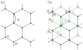
Figure 1: (Color online.) The lattice structure of (a) monolayer and (b) bilayer graphene annotated with the various hopping elements which are included in the tight-binding Hamiltonian. The dashed lines and larger unfilled circles denote the lower layer, the solid lines and smaller filled circles show the upper layer. Intra-layer and onsite elements are shown in black, inter-layer hops are drawn in green (gray).

The crystal structure of bilayer graphene consists of two monolayer lattices stacked such that the $A$ sublattice of the upper layer lies directly above the $B$ sublattice of the lower layer, separated by a distance $a_{z}$. This is called Bernal, or AB stacking and is illustrated in Fig. 1(b). A dimer bond is formed between these two lattices and is characterized by the energy $\gamma_{1}$ in the tight-binding Hamiltonian. In the bilayer, the sublattice asymmetries and next-nearest inter-layer hops do have a significant effect on the band structure and we describe the most relevant ones now. Firstly the layer potential asymmetry, which we denote by the energy $u$, breaks the inversion symmetry in the out-of-plane direction and lifts the degeneracy of the conduction and valence bands at the K points. Since this potential can be applied by gating, this generates a dynamically-tunable band gap [4, 5]. The hops between $A_{l}$ and $B_{u}$ lattices, parameterized by the energy $\gamma_{3}$ break the isotropy of the band structure reducing the symmetry from full rotational to C₃, and induce an overlap between the conduction and valence bands. The hops between $A_{l}$ and $A_{u}$ sublattices and between $B_{l}$ and $B_{u}$ sublattices parameterized by the energy $\gamma_{4}$ combine with the intra-layer potential asymmetry $\Delta$ to induce an asymmetry between the conduction and valence bands.

Using these notations, the Hamiltonian is

$$H^{b}=\begin{pmatrix}\tfrac{\xi u}{2}&\xi\hbar v_{3}\pi^{\dagger}&-\xi\hbar v_{4}\pi^{\dagger}&\xi\hbar v_{F}\pi^{\dagger}\\ \xi\hbar v_{3}\pi&-\tfrac{\xi u}{2}&\xi\hbar v_{F}\pi&-\xi\hbar v_{4}\pi\\ -\xi\hbar v_{4}\pi&\xi\hbar v_{F}\pi^{\dagger}&-\tfrac{\xi u}{2}+\Delta&\gamma_{1}\\ \xi\hbar v_{F}\pi&-\xi\hbar v_{4}\pi^{\dagger}&\gamma_{1}&\tfrac{\xi u}{2}+\Delta\end{pmatrix}$$ (4)

where the sublattice basis is $\{B_{u},A_{l},B_{l},A_{u}\}$ with $\xi=1$ in the K valley and $\{A_{l},B_{u},A_{u},B_{l}\}$ with $\xi=-1$ in the K^′ valley. The energies $\gamma_{3}$ and $\gamma_{4}$ give the velocities $v_{3,4}=\sqrt{3}\gamma_{3,4}a/(2\hbar)$. Figure 2 shows the band structure of bilayer graphene in three approximations. Solid lines denote the full solution of Eq. (4) with $\gamma_{0}=3.09\mathrm{eV}$, $\gamma_{1}=0.4\mathrm{eV}$, $\gamma_{3}=0.38\mathrm{eV}$, $\gamma_{4}=0.14\mathrm{eV}$, and $\Delta=0.022\mathrm{eV}$ where these values have been taken so that $v_{F}=10^{6}\mathrm{ms}^{-1}$ and $\gamma_{1}$ is in line with standard values taken in the literature. The higher order parameters were taken from an experimental study which extracted their values by fitting optical reflectivity spectra to the band structure of the full Hamiltonian [6]. Dashed lines indicate the spectrum when the asymmetry-inducing elements $\gamma_{4}$ and $\Delta$ are set to zero; and the dotted lines show the spectrum when the trigonal warping elements $\gamma_{3}$ are also set to zero. This final approximation is the most frequently used in the literature. Figure 2(a) shows the hyperbolic shape of the bands in the gapless case, and the asymmetries induced by the higher order tight binding parameters. Specifically, the trigonal warping terms push the bands towards positive $k_{x}$, and while it is not shown in the figure, this asymmetry causes the Fermi surface to become somewhat triangular, reducing its full isotropy to a three-fold rotational symmetry. The combined effect of $\gamma_{4}$ and $\Delta$ is to make the conduction band slightly steeper and the valence band somewhat shallower. We also include the linear dispersion of monolayer graphene for comparison, shown with the gray line. Figure 2(b) shows the same spectrum but with a gap generated by $u=100\mathrm{meV}$. The ‘sombrero’ shape near the K point is now noticeable, as is the distortion caused by the higher order tight binding terms which make the gap slightly narrower at the positive $k_{x}$ minimum. Figure 2(c) shows the low-energy region for the gapless case, and the overlap of the conduction and valence bands caused by $\gamma_{3}$ is now apparent. Figure 2(d) shows the same but for a small gap given by $u=10\mathrm{meV}$. Most of the complexity of the low energy band structure is encapsulated in this plot, including the distortion of the band edge and all the asymmetries described above.

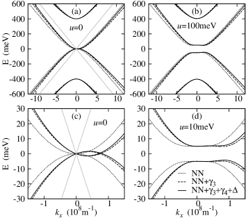
Figure 2: The bandstructure of bilayer graphene. (a) $u=0$ showing all four bands. (b) $u=100\mathrm{meV}$ showing all four bands. (c) Low-energy region for $u=0$. (d) Low-energy region for $u=10\mathrm{meV}$. The legend in (d) applies to all four panels, and ‘NN’ stands for nearest-neighbor. The gray line in (a) and (c) is the dispersion of monolayer graphene.

There is a common simplification of the bilayer Hamiltonian which is often used when only the very low density regime is under investigation [4]. By expanding the Green’s function of the Hamiltonian in Eq. (4) with respect to momentum, one can write down an effective two band Hamiltonian with quadratic dispersion. This effectively excludes the $A_{u}$ and $B_{l}$ sublattices from consideration, since electrons residing primarily on these sublattices form the split bands with energy $\sim\gamma_{1}$ near the K points and which are therefore not involved in low energy processes.

In order to derive exact expressions for $M$, we must first find an analytical expression for the density in terms of the chemical potential. Elementary considerations show us that the total number of electrons in the conduction band (or holes in the valence band) is related to the number of filled states as follows:

$$N=\sum_{\text{filled. st.}}1 =\frac{g_{s}g_{v}\mathcal{A}}{(2\pi)^{2}}\int f(\boldsymbol{\mathrm{k}})d^{2}\boldsymbol{\mathrm{k}}$$

$$\Rightarrow\qquad n =\frac{g_{s}g_{v}}{4\pi^{2}}\int_{0}^{2\pi}d\theta\int_{k_{F_{-}}(\theta)}^{k_{F_{+}}(\theta)}k\,dk$$

where $n=N/\mathcal{A}$, and the state occupancy at zero temperature is given by the function $f(\boldsymbol{\mathrm{k}})$ which takes the value 1 if the state with wave vector $\boldsymbol{\mathrm{k}}$ is occupied and 0 otherwise. The possible anisotropy and non-trivial topology of the band structure implies that the Fermi wave vector may be multiply-valued, and is a function of the angle $\theta$. The factors $g_{s}$ and $g_{v}$ are for spin and valley degeneracies, respectively, and both take the numerical value of 2. Evaluating the radial part gives

$$n=\frac{g_{s}g_{v}}{8\pi^{2}}\int_{0}^{2\pi}d\theta\left(k_{F_{+}}^{2}(\theta)-k_{F_{-}}^{2}(\theta)\right)$$ (5)

This integral equation (which depends on the chemical potential via the Fermi wave vectors) can now be evaluated to give an expression for $\mu$ in terms of $n$. This can then be differentiated with respect to $n$ to give $M$.

This process can be carried out analytically in a number of cases. For monolayer graphene, the Fermi surface is always circular such that $k_{F_{-}}(\theta)=0$ and $k_{F_{+}}(\theta)=k_{F}$. Then, Eq. (5) becomes

$$n=\frac{g_{s}g_{v}}{8\pi^{2}}\int_{0}^{2\pi}d\theta\left(k_{F}^{2}-0\right)=\frac{k_{F}^{2}}{\pi}\quad\Rightarrow\quad k_{F}^{2}=\pi n.$$ (6)

The band structure also gives us $\mu=\hbar v_{F}k_{F}=\hbar v_{F}\sqrt{\pi n}$ so that

$$M^{m}=\frac{\hbar v_{F}\sqrt{\pi}}{2\sqrt{n}}.$$ (7)

Similarly, the quadratic band structure yields a constant value for $M$:

$$M^{q}=\frac{\hbar^{2}v_{F}^{2}\pi}{\gamma_{1}}.$$ (8)

The four-band model for bilayer graphene with $\gamma_{3}=\gamma_{4}=\Delta=0$ also gives an analytical result. However, in this case, the Fermi energy may be ring-shaped for low density, and for high density both the low-energy and split bands are populated. Therefore $M$ shows two step-like features as the Fermi energy moves between these regions:

$$M^{h}=\frac{\gamma_{1}u}{\sqrt{g_{u}}}\delta(n)+\frac{\hbar^{2}v_{F}^{2}\pi}{2}\begin{cases}\frac{\lambda}{\sqrt{g_{u}}}\frac{1}{\sqrt{\lambda^{2}+u^{2}\gamma_{1}^{2}}}&\lambda<u^{2}\\ \frac{1-g_{u}/\left(2\sqrt{\lambda g_{u}+\gamma_{1}^{4}/4}\right)}{\sqrt{\lambda+\frac{u^{2}}{4}+\frac{\gamma_{1}^{2}}{2}-\sqrt{\lambda g_{u}+\frac{\gamma_{1}^{4}}{4}}}}&u^{2}\leq\lambda<2\gamma_{1}^{2}+u^{2}\\ \frac{1}{\sqrt{2\lambda+u^{2}}}&\lambda\geq 2\gamma_{1}^{2}+u^{2}\end{cases}$$ (9)

where we use the notation $g_{u}=\gamma_{1}^{2}+u^{2}$ for brevity. The first term of this expression which contains the $\delta$-function is present because in the gapped case, a discontinuity exists in the chemical potential at the band edge: for an infinitesimal change in density, the chemical potential jumps from the valence band to the conduction band, and differentiating this step gives the $\delta$ function as shown. Including the higher-order tight binding elements means that analytical solutions are no longer possible, and numerical evaluation must be conducted instead.

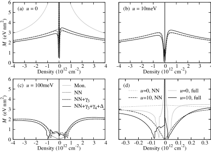
Figure 3: $M=d\mu/dn$ for clean bilayer graphene. (a) The gapless case, also with $M^{m}$ for monolayer graphene. (b) $u=10\mathrm{meV}$, and (c) $u=100\mathrm{meV}$. The legend in (c) shows the approximation for the bilayer Hamiltonian used in each case and applies to panels (a)–(c). (d) Low-density region for the full Hamiltonian and three different gap values (corresponding to the solid lines from the other three panels).

Figure 3 shows $M$ in the various cases we have described. We point out the important features. Firstly, in the gapless case, shown in Fig. 3(a), the monolayer (gray line) $M$ is substantially larger than the bilayer and diverges as $1/\sqrt{n}$ as $n\to 0$. In the NN approximation for the bilayer, $M$ goes smoothly to the finite value $\hbar^{2}v_{F}^{2}\pi/\gamma_{1}$ at $n=0$. The decrease in $M$ at finite density reflects the non-parabolicity of the band structure. When the second-order hopping elements are included, a sharp peak is present at $n=0$ with dips at small density on either side. This is due to the change in topology of the Fermi surface with finite $\gamma_{3}$ and the region where $M$ decreases relative to the NN case corresponds to the density range where Fermi surface has split into four pockets. At high density, the asymmetry induced by the combination of $\gamma_{4}$ and $\Delta$ manifests as a reduction in $M$ for the valence band and enhancement for the conduction band. This also reveals that the presence or absence of $\gamma_{3}$ from the Hamiltonian has little effect at higher density. When a small gap is opened, shown in Fig. 3(b) for $u=10\mathrm{meV}$, the divergence in the density of states at the band edge manifests as $M\to 0$ when $n\to 0$. However, we illustrate the $\delta$-function spike as an infinitesimally wide divergence exactly at $n=0$. The effect of the trigonal warping is now masked by the band gap and the asymmetry between the conduction and valence bands is unmodified. When the gap is wider, shown for $u=100\mathrm{meV}$ in Fig. 3(c), there is an extended range of density (approximately $|n|<10^{12}\mathrm{cm}^{-2}$) where the Fermi energy is in the sombrero region. For the NN approximation, $M$ is linear, but for the higher order approximations of the Hamiltonian, the non-isotropic band structure creates a rather complex shape for $M$. In Fig. 3(d) we show the low-density region for the gapless and gapped ($u=10\mathrm{meV}$) cases, for the NN and full approximations for the band structure. This shows the dip–peak structure in the gapless full approximation more clearly, in addition to the complexity of $M$ in the gapped full approximation.

Finally, we note that this single particle analysis has been used to compare the quantum capacitance of bulk monolayer graphene to that of graphene nanoribbons [7].

2 Electron–electron interactions

We now consider the effect of direct Coulomb interactions between electrons and correlations on the compressibility. The first observation [8] is that in the absence of direct electron–electron interactions, the kinetic energy part of the correlation (an expression of the fact that electrons are fermionic) between two electrons behaves qualitatively differently for monolayer and bilayer graphene. Specifically, the two-particle correlation cancels exactly for monolayer (leaving only the contribution from the trivial single particle kinetic energy part) whereas it remains finite for the bilayer. This is due to the differences in the chirality of the two electron liquids. This cancellation in the correlation implies that the compressibility is determined by only the single particle kinetic energy, as seen in experiments [9]. In contrast, the bilayer does not show this cancellation, implying that correlations and the contribution from the interactions are likely to play a more significant role in that material.

To take into account the effects of interactions between electrons, various levels of approximation have been employed. At the Hartree–Fock level in monolayer graphene [10], the renormalized $M$ retains the $n^{-1/2}$ dependence of the non-interacting system, but the value of $M$ is increased relative to the non-interacting electrons. The overall enhancement in the extrinsic case is approximately 20% when the parameters relevant for graphene mounted on an SiO₂ substrate are used. The authors also showed that the renormalization is increased when the dielectric environment of the graphene is weaker, suggesting that the enhancement of $M$ will be stronger in suspended graphene. At the RPA level with finite doping, interactions between electrons favor states with large chirality [11] which leads to a suppression of both charge and spin susceptibilities. In this approximation, the overall sign of the compressibility remains positive but the interactions reduce it by up to a factor of 2 corresponding to an enhancement of $M$, depending on the strength of the coupling constant (which is defined by the environment of the graphene) and the value of an arbitrarily defined momentum cutoff. For physically realistic parameters, a suppression of $\kappa\propto 1/M$ of $15\%$ is predicted.

In contrast, the introduction of electron–electron interactions at the Hartree–Fock level to ungapped bilayer graphene [12] gives a profound change to the predicted inverse compressibility (proportional to $M$) because at low carrier density it becomes negative and divergent. Just as in the monolayer, the contributions from the intra-band and inter-band terms are opposite in sign, but in the case of the bilayer at low density, the inter-band terms (which are negative) are stronger which leads to a negative divergence as $n\to 0$. For the monolayer, the (negative) inter-band terms are never strong enough to overcome the (positive) intra-band contribution. Also, while the two-band model provides a reasonable approximation for $M$ at low densities, the authors point out that the full four-band model is required at intermediate and higher densities. If the RPA approximation to the correlation part of the exchange is included [13] then the negative divergence is removed because the contribution to the total energy per particle given by the correlation effects cancels the decreasing contribution from the exchange implying that $M$ is always positive. The compressibility $\kappa$ is reduced with respect to the non-interacting case, but this enhancement of $M$ reduces with increasing carrier density.

Finally, we mention in passing that the compressibility may be a useful tool for investigating the nature of the ground state of charge-neutral (intrinsic) bilayer graphene. There have been many theoretical works (Refs. [14] and [15] are two of the earliest) which suggest that this system is unstable against transitions to various broken-symmetry phases. The nematic phase and anomalous Hall insulator are two of the strongest candidates, and may lead to distinctive behavior of $M$ and $\kappa$ at low density. In fact, some experiments [16] have already been interpreted in this manner.

3 Disorder

3.1 Introduction

The effect of disorder is known to be crucial for determining many observable properties of graphene materials, and in many cases may mask the effects of electron–electron interactions discussed above. For example, the Dirac point physics can be completely masked by charge inhomogeneity [9] and in the more dirty samples, the presence of the externally tunable band gap in bilayer graphene can be obscured in transport measurements [17]. The exact cause of the charge inhomogeneity (which manifests as ‘puddles’ at low average carrier density) is still somewhat controversial, so below we briefly outline the proposed mechanisms and proceed to assume the existence of the charge inhomogeneity as a phenomenological reality and discuss its impact on the compressibility.

Before discussing the effects of puddles, we mention that for monolayer graphene, the effect of a finite scattering rate between the electrons and charged impurities, the effect of ripples, and a contribution from the correlation between electrons have been examined [18], and good agreement between the RPA theory and experimental data was found at higher density. However, at low density the theory does not modify the single-particle behavior (a divergence as $n\to 0$) in contrast to the experimental data.

3.2 The effect of puddles

The ‘puddles’ of carriers were first observed in monolayer graphene via scanning SET microscopy [9] and subsequently in STM measurements for monolayer [19] and bilayer [20, 21] graphene. The conventional wisdom is that these puddles are caused by external charged impurities (either located in the substrate, at the interface between the substrate and the graphene, or on top of the graphene) which have an electric field associated with them. This field produces a spatially fluctuating potential which the electrons experience as a shift in the band structure relative to the Fermi energy which in turn modifies the number of carriers in that locality. This idea has been used theoretically to predict the size and distribution of these puddles [22, 23, 24], and these studies agree qualitatively with the experimental measurements for both monolayer and bilayer graphenes. Recently, another theory has been advanced [25] which suggests that the scalar and vector potentials induced by corrugations in the graphene sheet may also cause puddles to form. The authors use a continuum elasticity theory for the graphene sheet and self-consistent Kohn–Sham–Dirac theory to calculate the induced carrier density. They find that there is no obvious correlation between the corrugations and the puddle landscape and state that this is due to the non-local relation between the corrugation-induced scalar potential and the tensor field due to height fluctuations. Other work [26] has also hinted at a link between charge inhomogeneity and deformations of the graphene sheet since the rippling of monolayer graphene on a substrate gives rise to a gauge field which may cause low-energy Landau levels to form, accompanied by an increase in $M$ at low density.

A phenomenological theory which accounts for puddles has been developed [27, 28] for incorporating the effects of disorder in calculations of $M$. For a measurement technique which simultaneously samples an area large enough to encompass several puddles (such as a bulk capacitance probe which samples the whole area between the gates, or an SET tip which samples an area with radius $\sim 100\mathrm{nm}$) and which couples capacitively to the electronic liquid in the graphene, it is sensible to assume that the measured response is the average over the sampled area. The idea is that each area with similar density will act as an independent capacitor and that $M$ will be set by that density. Hence the total of all these parallel regions is their average and this suggests that the areal average can be replaced by an average over the density distribution $P$. In order to model this distribution we write the total local density $n(\boldsymbol{\mathrm{r}})=n_{0}+\tilde{n}(\boldsymbol{\mathrm{r}})$ where $n_{0}$ is the average density which in an experiment is set by the external gates, and $\tilde{n}(\boldsymbol{\mathrm{r}})$ is the spatially fluctuating part induced by the disorder potential. We also assume that the density distribution is described by one parameter—a measure of the average fluctuation which we label $\delta n$. The average value of $M$, which we denote $\bar{M}$ is

$$\bar{M}(n_{0},\delta n,u)=\int_{-\infty}^{\infty}M(n,u)P(n,n_{0},\delta n)dn$$ (10)

Note that this procedure contains an uncontrolled approximation that the Bloch states used in the derivation of $M$ persist in the disordered context and may be used as a basis over which to perform the average. Since the density inhomogeneity breaks translational invariance, this is not strictly true. Also, for monolayer graphene, this procedure is not completely defined because the $n^{-1/2}$ divergence in $M$ at low density means that the integral is infinite. However, an artificial cutoff could be introduced to rectify this. The $\delta$-function divergence in the gapped bilayer is integrable and hence provides no technical difficulty.

In the case of bilayer graphene, this procedure has been used to fit experimental data with a high degree of accuracy [27, 28] despite the phenomenological nature of the theory. To illustrate this, Fig. 4 shows $\bar{M}$ for different disorder strengths, different values of the gap, and for several combinations of the tight binding elements $\gamma_{3}$, $\gamma_{4}$, and $\Delta$. It is known both experimentally [29] and theoretically [23] that $P$ is Gaussian for bilayer graphene and so we write

$$P(n,n_{0},\delta n)=\frac{1}{\sqrt{2\pi}\delta n}\exp\left[-\frac{(n-n_{0})^{2}}{2\delta n^{2}}\right]$$

As representative values of the density fluctuations, we take $\delta n=10^{11}\mathrm{cm}^{-2}$ to stand for graphene on an SiO₂ substrate, and $\delta n=10^{10}\mathrm{cm}^{-2}$ for both suspended graphene and graphene on an $h$BN substrate. According to the literature, these constitute rather conservative estimates of the density inhomogeneity. In Fig. 4(a) we show $\bar{M}$ for strongly disordered bilayer graphene in a wide density range. At higher density, the averaging procedure has very little effect and $\bar{M}$ is almost unchanged from $M$. But at low density the sharp dips in $M$ (see Fig. 3) become smoothed out into a small dip in $\bar{M}$ near $n=0$. When the disorder is much weaker, as shown in Fig. 4(b), the sequence of dips and central peak at $n=0$ is restored (notice the different scale on the horizontal axis in this panel). When a small gap is opened, the extra complexity in $M$ in the low density regime is obscured by the wide sampling region for strongly disordered samples, as shown in Fig. 4(c). But for smaller disorder, Fig. 4(d), the sequence of dips on either side of the $n=0$ peak are discernable. In the case of the wide gap with large disorder, Fig. 4(e), the effect of the second-order tight-binding elements is obscured and the most important factor determining the shape is the broadened $\delta(n)$ term.

In conclusion, the effect of the puddles on $M$ at low carrier density in bilayer graphene is an intricate quantitative question in which two main effects – the size of the layer asymmetry $u$, and the size of the density fluctuations – both play an important role. Additionally, the shape of $\bar{M}$ is qualitatively different in the gapless case, and quantitatively different in the presence of a gap, depending on the approximation taken for the tight-binding Hamiltonian.

Figure 4: Effect of averaging procedure $\bar{M}$. All lines correspond to the legend in (a) (where ‘NN’ stand for nearest-neighbor), and the parameters used in each panel are shown in the accompanying table.

3.3 Spatial fluctuation in band gap

It has been observed in experiments for graphene on single-gated SiO₂ [20] that the size of the inter-layer potential asymmetry (the parameter $u$ in the tight-binding formalism, which sets the size of the band gap) may fluctuate in space. Specifically, these authors fitted $dI/dV$ maps of bilayer graphene in a strong magnetic field to the single particle Landau level spectrum and were able to extract both the magnitude and sign of $u$. They found variation on the order of tens of meV, and that the orientation of the asymmetry swapped between electron puddles and hole puddles. The spatial fluctuation of the gap was implemented in this phenomenological theory [28] to model the low-density region of suspended bilayers by assuming that the local gap could be written $u(\boldsymbol{\mathrm{r}})=u_{0}+\tilde{u}(\boldsymbol{\mathrm{r}})$ in an analogous way to the density fluctuations with $\delta u$ parameterizing the fluctuations in $\tilde{u}$. Then, a second averaging procedure can be performed over the distribution of $\tilde{u}$ yielding

$$\bar{\bar{M}}=\int_{-\infty}^{\infty}\bar{M}(n_{0},\delta n,u)P(u,u_{0},\delta u)du$$ (11)

It was found that for these suspended samples, it was not possible to distinguish clearly between a gap formed by spontaneous electron–electron interaction effects (which is encapsulated in a finite $u_{0}$) and a disorder-induced gap modeled by finite $\delta u$. This is summarized in Fig. 5 where the best fits from the theories for fluctuating gap ($\bar{\bar{M}}$) and homogeneous gap ($\bar{M}$) are compared to experimental data for two samples. Therefore, if possible, measurements of $M$ in samples with even less disorder are required to unambiguously determine the magnitude of the intrinsic gap.

Figure 5: Comparison between gap formation mechanisms in comparison to experiments.

4 Experiments

Experimental determinations of $M$ or the compressibility of graphene have been made via scanning SET microscopy [9, 16], and bulk capacitance measurements [30, 31]. In the case of monolayer graphene [9], the measured $M$ is close to the single particle result with a Fermi velocity of $1.1\times 10^{6}\mathrm{ms}^{-1}$. This corresponds to the theoretical result where the $1/\sqrt{n}$ divergence persists in the presence of disorder with a renormalization of the Fermi velocity. The effects of disorder at low density are noticeable as a cutting off of the divergence as $n\to 0$.

There have been more experiments done on bilayer graphene. In Refs. [30, 31] $M$ is extracted from bulk capacitance measurements of dual-gated bilayer sheets in close contact to the gates. This geometry induces a large degree of disorder from charged impurities and the dominant effects shown in these experiments are the broadening of features due to the puddle averaging described in Section 3.2. The asymmetry between the electron and hole bands caused by $\gamma_{4}$ and $\Delta$ are also clearly seen in [30]. In contrast, scanning SET microscopy of suspended bilayer graphene [16] accesses much cleaner samples. It is claimed that the increase in $M$ measured near $n=0$ in these experiments comes from the formation of a broken symmetry ground state such as a nematic phase [14] or an anomalous Hall insulator [15]. However, other features in the theory described in Section 2 (such as the negative divergence of $\kappa^{-1}$ in the ungapped bilayer, or quantitative estimates of the size of the renormalization of $M$ due to electron–electron interactions) have not been observed.

5 Conclusions and discussion

The compressibility of an electron liquid and its related quantities $M=d\mu/dn$ and the quantum capacitance are important objects of study in condensed matter physics since they give information about the intrinsic nature of the electron liquid and its interactions with external fields. In this review, we have described the band structure and detailed features of $d\mu/dn$ in monolayer and bilayer graphene, including the effects of electron–electron interactions and disorder. We have also reviewed the current status of experimental work. The single particle picture for $d\mu/dn$ is rather clear for monolayer graphene and for bilayer graphene at high carrier density. But for the bilayer in the low density limit, there are qualitative differences between the various commonly used approximations to the Hamiltonian. In particular, when the next-nearest neighbor hoppings are included in the gapless case, significant additional structure appears at experimentally relevant density. Comparison with current experiments shows that disorder (specifically, the existence of inhomogeneity in the charge density landscape) is the dominant source of deviations from the single particle picture in graphene samples in contact with a substrate, while in suspended samples it is possible that the interaction effects are being observed.

We gratefully acknowledge support from US-ONR, NRI-SRC-SWAN, and LPS-NSA.

References

- [1] D. S. L. Abergel, V. Apalkov, J. Berashevich, K. Ziegler, T. Chakraborty, Adv. Phys. 59 (2010) 261.
- [2] S. Das Sarma, S. Adam, E. H. Hwang, E. Rossi, Rev. Mod. Phys. 83 (2011) 407.
- [3] A. H. Castro Neto, F. Guinea, N. M. R. Peres, K. S. Novoselov, A. K. Geim, Rev. Mod. Phys. 81 (2009) 109.
- [4] E. McCann, V. I. Fal’ko, Phys. Rev. Lett. 96 (2006) 086805.
- [5] E. McCann, Phys. Rev. B 74 (2006) 161403.
- [6] A. B. Kuzmenko, I. Crassee, D. van der Marel, P. Blake, K. S. Novoselov, Phys. Rev. B 80 (2009) 165406.
- [7] T. Fang, A. Konar, H. Xing, D. Jena, Appl. Phys. Lett. 91 (2007) 092109.
- [8] D. S. L. Abergel, P. Pietiläinen, T. Chakraborty, Phys. Rev. B 80 (2009) 081408.
- [9] J. Martin, N. Akerman, G. Ulbricht, T. Lohmann, J. H. Smet, K. von Klitzing, A. Yacoby, Nat. Phys. 4 (2008) 144.
- [10] E. H. Hwang, B. Y.-K. Hu, S. Das Sarma, Phys. Rev. Lett. 99 (2007) 226801.
- [11] Y. Barlas, T. Pereg-Barnea, M. Polini, R. Asgari, A. H. MacDonald, Phys. Rev. Lett. 98 (2007) 236601.
- [12] S. V. Kusminskiy, J. Nilsson, D. K. Campbell, A. H. Castro Neto, Phys. Rev. Lett. 100 (2008) 106805.
- [13] G. Borghi, M. Polini, R. Asgari, A. H. MacDonald, Phys. Rev. B 82 (2010) 155403.
- [14] O. Vafek, K. Yang, Phys. Rev. B 81 (2010) 041401.
- [15] F. Zhang, H. Min, M. Polini, A. H. MacDonald, Phys. Rev. B 81 (2010) 041402.
- [16] J. Martin, B. E. Feldman, R. T. Weitz, M. T. Allen, A. Yacoby, Phys. Rev. Lett. 105 (2010) 256806.
- [17] J. B. Oostinga, H. B. Heersche, X. Liu, A. F. Morpurgo, L. M. K. Vandersypen, Nat. Mater. 7 (2008) 151.
- [18] R. Asgari, M. M. Vazifeh, M. R. Ramezanali, E. Davoudi, B. Tanatar, Phys. Rev. B 77 (2008) 125432.
- [19] A. Deshpande, W. Bao, F. Miao, C. N. Lau, B. J. LeRoy, Phys. Rev. B 79 (2009) 205411.
- [20] G. M. Rutter, S. Jung, N. N. Klimov, D. B. Newell, N. B. Zhitenev, J. A. Stroscio, Nat. Phys. 7 (2011) 649.
- [21] A. Deshpande, W. Bao, Z. Zhao, C. N. Lau, B. J. LeRoy, Appl. Phys. Lett. 95 (2009) 243502.
- [22] E. Rossi, S. Das Sarma, Phys. Rev. Lett. 101 (2008) 166803.
- [23] E. Rossi, S. Das Sarma, Phys. Rev. Lett. 107 (2011) 155502.
- [24] S. Adam, S. Jung, N. N. Klimov, N. B. Zhitenev, J. A. Stroscio, M. D. Stiles, Phys. Rev. B 84 (2011) 235421.
- [25] M. Gibertini, A. Tomadin, F. Guinea, M. I. Katsnelson, M. Polini, ArXiv e-prints arXiv:1111.6280.
- [26] F. Guinea, M. I. Katsnelson, M. A. H. Vozmediano, Phys. Rev. B 77 (2008) 075422.
- [27] D. S. L. Abergel, E. H. Hwang, S. Das Sarma, Phys. Rev. B 83 (2011) 085429.
- [28] D. S. L. Abergel, H. Min, E. H. Hwang, S. Das Sarma, Phys. Rev. B 84 (2011) 195423.
- [29] K. Burson, et al., (2011), (unpublished).
- [30] E. A. Henriksen, J. P. Eisenstein, Phys. Rev. B 82 (2010) 041412.
- [31] A. F. Young, L. S. Levitov, Phys. Rev. B 84 (2011) 085441.