Non-Extremality, Chemical Potential and the Infrared limit of Large $N$ Thermal QCD

Abstract:

Non-extremal solution with warped resolved-deformed conifold background is important to study the infrared limit of large $N$ thermal QCD. Earlier works in this direction have not taken into account all the back-reactions on the geometry, namely from the branes, fluxes, and black-hole carefully. In the present work we make some progress in this direction by solving explicitly the supergravity equations of motions in the presence of the backreaction from the black-hole. The backreactions from the branes and the fluxes on the other hand and to the order that we study, are comparatively suppressed. Our analysis reveal, among other things, how the resolution parameter would depend on the horizon radius and how the RG flows of the coupling constants should be understood in these scenarios, including their effects on the background three-form fluxes. We also study the effect of switching on a chemical potential in the background and, in a particularly simplified scenario, compute the actual value of the chemical potential for our case.

1 Introduction

Much of what is known about the phases of strongly coupled gauge theories (and in particular, QCD) comes from a variety of techniques, each of which accompanied by its attendant limitations. Perturbative (i.e. weak coupling) computations can probe a large part of the parameter space of the theory, like allowing one to deal with varying number of colors $N$, flavors $N_{f}$. However, these results are valid only at temperatures well above the deconfinement temperature $T_{c}$, and at large values of the baryon number chemical potential $\mu$ in order for the QCD coupling to be small, and thus the perturbation valid. These exclusions put almost all of the interesting region of the parameter space explored by RHIC data beyond the reach of perturbative computations.

Lattice gauge theory, which provides a rigorous non-perturbative starting point for QCD, is not without its limitations as well. It is difficult to incorporate realistic quark masses, and results from the traditional lattice simulations are limited to the regime near $T_{c}$, and $\mu$ very small. Nonetheless, a combination of such conventional methods of analysis (including insights from effective theories like chiral models) suggest that the gauge theory possesses a color superconductivity phase at asymptotically large value of the baryon number chemical potential $\mu$. The literature is replete with conjectures for the phase diagram of QCD in the ($T,\mu$) plane, especially for small values of $T$ and large values of $\mu$ (see for example [2, 1]).

In recent years, there has been a considerable advance in understanding the behavior of $U(N)$ gauge theories at finite temperature using the gauge/gravity duality. That this development is more than timely is beyond dispute, as the new and interesting results from RHIC have provided a glimpse into a wide variety of interesting phenomena arising in the strong coupling regime of QCD. For instance, the quark-gluon plasma (identified as a new state of matter) displays many properties of a fluid with low (shear) viscosity, explanations for which are difficult to obtain from traditionally available tools in perturbative QCD.

Many (perhaps most!) analytic results coming from gauge-gravity duality are derived for gauge theories with ${\cal N}=4$ supersymmetry and with $N$ very large, and in the limit of the theory possessing exact conformal symmetry. One may thus genuinely be concerned about their applicability to QCD for which all these are not true. Recent progress in this area, however, has provided us with strong hints to overcome these limitations, and move towards models of gauge-gravity duality that are not supersymmetric, and are non-conformal (in a sense that will be made precise later).

The first set of models that managed to expand the original AdS/CFT construction to incorporate renormalization group runnings are [9, 10] that connected conformal fixed points at IR and UV, and [11] that connected the UV ${\cal N}=4$ conformal fixed point to a ${\cal N}=1$ confining theory. The next set of models, that we would be mostly interested in, do not have any fixed points (or fixed surfaces) in the paths of the RG flows. The key example in this set is the Klebanov-Strassler (KS) model [12] (with an extension by Ouyang [13] to incorporate fundamental matters) that provided an IR dual of, although not exactly QCD, but at least its closest cousin: large $N$ supersymmetric QCD. The UV of the original Klebanov-Strassler model is now known to have some issues, like the divergences of the Wilson loops at high energies, and additional Landau poles once fundamental matters have been introduced. This means that UV completion is necessary, and to have the full gravity dual of the corresponding gauge theory that behaves well at high energies, the KS geometry has to be augmented by a proper asymptotic manifold.

Other extensions to the original KS model quickly followed. For example in [23, 15] the cascading picture of the original KS model was extended to incorporate black-hole without any fundamental matter, which was then further extended to incorporate matter in [16]. However none of the above models actually considered the full UV completion as most of the analysis of these works were directed towards unravelling the IR physics. Therefore issues like UV divergences of Wilson loops and Landau poles were not investigated.

In a series of works [6, 25, 30, 27] done over the last couple of years, we tried to address these concerns. Our aim therein was to incorporate the backreactions from the black-hole, fluxes, and branes consistently so as to have a well defined UV completion that not only allow us to get rid of all the poles etc., but also give us a model that could come closest to what we might have expected from a large $N$ thermal QCD. We did manage to at least successfully generate such a UV completed dual picture, but many of the backreactions turned out to be too difficult to incorporate fully. One aim of this paper is to make progress in this direction. In sec. 2.1 we will show how exactly to incorporate the backreactions from the black-hole in IR regime of our theory to lowest orders in string coupling, and color-to-flavor ratio. Interestingly, to this order, the backreactions from branes and fluxes could be consistenly ignored. We will demonstrate this in sec. 2.1.1, and relevant EOMs will be solved in sec. 2.1.2 and in Appendix C.

Although to the order that we study the IR regime of our theory allows us to ignore the backreactions of the fluxes, we will in-fact work out the detailed fluxes in sec. 2.2. The backreactions from the black hole and the flavor seven-branes will be fully incorporated in the fluxes. It will also be clear from sec. 2.2 as to how these backreactions conspire to make the three-form fluxes non-ISD.

One persistent problem associated with thermal QCD is the interpretation of beta function of the theory. There is a long history on the subject starting with the classic work by Collins and Perry [19]. In sec. 2.3 we discuss briefly how we should interpret the running of couplings from the gravity dual. Our work strongly suggest one framework, although alternative interpretation could possibly be entertained.

We end sec. 2 by taking a short detour. In sec. 2.4 we study the dipole and non-commutative deformations of the seven-brane theory on the gravity side. This detour is not without its merit. Dipole deformations are known to increase the masses of the KK states, so that a dipole-deformed theory will have a slightly different KK spectra. We again make very brief speculations of the underlying physics, leaving most of the details for future work.

Thus sec. 2 prepares us with a backreacted metric, and with backreacted fluxes. One may now go on with this to fill up rest of the missing steps left in [6, 25, 30, 27]. These issues however will be addressed in future works. Here we aim for more modest return. In sec. 3 we present a small computation on the chemical potential. The reason for choosing this computation over other possible interesting ones is two-fold. One: its simple enough computation that carries sufficiently interesting physics, and two: we use this to show in sec. 3.2 how an alternative way of getting the chemical potential, via say duality chasing, may be inherently flawed. In sec. 3.3 we compute the chemical potential for our model. In Appendices A, and B we speculate more on the duality chasing techniques. We conclude in sec. 4 with some discussions.

2 Analysis of the background

Before discussing the details of the UV complete dual geometry, let us first review the Klebanov-Tseytlin (KT), Klebanov-Strassler (KS) and Ouyang-Klebanov-Strassler (OKS) geometry without the black hole. The supergravity description arises as the low energy limit of brane excitations placed in conifold geometry. In particular, the Klebanov-Tseytlin geometry arises from the following brane configuration: Embed $N$ D3 branes and $M$ D5 branes in ten dimensional manifold with the metric

$$ds_{10}^{2}=-dt^{2}+d\overrightarrow{x}^{2}+ds_{6}^{2}$$ (1)

where $ds_{6}^{2}$ is given by

$$ds^{2}_{6}=dr^{2}+r^{2}ds^{2}_{T^{1,1}}$$ (2)

The metric of the base $T^{1,1}$ is given by

$$ds^{2}_{T^{1,1}}=\frac{1}{9}\left[d\psi+\sum_{i=1}^{2}{\rm cos}\theta_{i}d\phi_{i}\right]^{2}+\frac{1}{6}\sum_{i=1}^{2}\left[d\theta_{i}^{2}+{\rm sin}^{2}\theta_{1}d\phi_{i}^{2}\right]$$ (3)

That is we have four dimensional Minkowski space along with six dimensional conifold. The D3 branes live in the flat four dimensional space and and are placed at the tip of the conifold at fixed radial location $r=0$. The D5 branes wrap the shrinking two cycle $S^{2}$ at the tip of the conifold and extend in four Minkowski directions.

The excitations of the massless open strings ending on these D branes are described by gauge fields and complex matter fields $A_{i},B_{i}$, $i=1,2$ which transform as bi-fundamental fields under the gauge group $SU(N+M)\times SU(N)$. Note that the matter fields $A_{1},A_{2}$ transform under global $SU(2)$ and so do $B_{1},B_{2}$ under another $SU(2)$ and we also have global $U(1)$ phase rotation. Thus we have $SU(2)\times SU(2)\times U(1)$ global symmetry, which is also the symmetry of the conifold.This is not surprising as these fields describe motion of the D branes [7] and the branes move in the conifold direction. Thus the fields $A_{i},B_{i}$ are really coordinates of the conifold

At the lowest energies, the entire setup of branes and their interaction with the gravitons can be captured by supergravity with only fluxes and metric and no branes. This geometry arising from supergravity is referred to as the dual geometry. For the brane configuration just described, the dual geometry is the warped regular cone with the following metric

$$ds^{2} = {1\over\sqrt{h_{\rm KT}}}\left(-dt^{2}+dx^{2}+dy^{2}+dz^{2}\right)+\sqrt{h_{\rm KT}}\Big{[}dr^{2}+r^{2}ds^{2}_{T^{1,1}}\Big{]}$$

$$h_{\rm KT} = \frac{L^{4}}{r^{4}}\Bigg{[}1+\frac{3g_{s}M^{2}}{2\pi N}{\rm log}r\Bigg{]}$$ (4)

The above warped geometry is known as the Klebanov-Tseytlin (KT) solution [8]. Right away, one observes that the warp factor $h_{\rm KT}$ becomes negative for small $r$ and the geometry is not well defined. In fact classical gravity description breaks down for small $r$ and the solution (2) is only valid for large $r$.

Since $r$ is related to the energy scale of the gauge theory, to understand what happens for small $r$, we can look at the IR limit of the gauge group $SU(N+M)\times SU(N)$. If $N=kM$, $k$ is a natural number, then at the IR, the gauge theory cascades down to $SU(M)$ under a Seiberg duality cascade. At the IR, the gauge theory develops a non-perturbative superpotential and the vacuum solution gives non-trivial expectation values for the gauge invariant operator $N_{ij}=A_{i}B_{j},i,j=1,2$. This means ${\rm det}N_{ij}=\epsilon^{2}\neq 0$. Since $A_{i},B_{j}$ are also cone coordinates, ${\rm det}N_{ij}=\epsilon^{2}$ also gives the cone embedding equation. However, $\epsilon\neq 0$ just means we no longer have a regular cone, but a deformed cone. This way the field theory analysis indicates that the dual geometry must be a deformed cone.

Thus to resolve the small $r$ singularity of the metric (2), we must replace the warped regular cone with the deformed warped cone. This is the essence of the Klebanov-Strassler (KS) proposal [12] and the dual geometry of the warped deformed cone has the following metric:

$$ds^{2} = \frac{1}{\sqrt{h_{\rm KS}}}\Big{[}-dt^{2}+dx^{2}+dy^{2}+dz^{2}\Big{]}+\sqrt{h_{\rm KS}}\;\bar{g}_{mn}dx^{m}dx^{n}$$

$$h_{\rm KS}(\rho) = \alpha\frac{2^{2/3}}{4}\int_{\rho}^{\infty}dx\frac{x\;{\rm coth}x-1}{{\rm sinh^{2}x}}\left({\rm sinh}(2x)-2x\right)^{1/3}$$ (5)

where $\alpha={\cal O}(g_{s}^{2}M^{2})$ and $\bar{g}_{mn}$ is the metric of the deformed cone

$$\bar{g}_{mn}dx^{m}dx^{n}~{}=\frac{1}{2}a^{4/3}K(\rho)\Big{[}\frac{1}{3K^{3}(\rho)}\left(d\rho^{2}+(g^{5})^{2}\right)+{\rm cosh}^{2}\left(\frac{\rho}{2}\right)\left[(g^{3})^{2}+(g^{4})^{2}\right]$$

$$+{\rm sinh}^{2}\left(\frac{\rho}{2}\right)\left[(g^{1})^{2}+(g^{2})^{2}\right]\Big{]}$$ (6)

where $a$ is a constant, $g^{i},i=1,..,5$ are one forms given by

$$g^{1}=\frac{e^{1}-e^{3}}{\sqrt{2}},~{}~{}~{}~{}g^{2}=\frac{e^{2}-e^{4}}{\sqrt{2}}$$

$$g^{3}=\frac{e^{1}+e^{3}}{\sqrt{2}},~{}~{}~{}~{}g^{4}=\frac{e^{2}+e^{4}}{\sqrt{2}},~{}~{}~{}g^{5}=e^{5}$$

$$e^{1}\equiv-{\rm sin}\theta_{1}\;d\phi_{1},~{}~{}~{}~{}e^{2}\equiv d\theta_{1}$$

$$e^{3}\equiv{\rm cos}\psi\;{\rm sin}\theta_{2}\;d\phi_{2}-{\rm sin}\psi\;d\theta_{2},$$

$$e^{4}\equiv{\rm sin}\psi\;{\rm sin}\theta_{2}\;d\phi_{2}+{\rm cos}\psi\;d\theta_{2},$$

$$e^{5}\equiv d\psi+{\rm cos}\theta_{1}\;d\phi_{1}+{\rm cos}\theta_{2}\;d\phi_{2}$$ (7)

and $K(\rho)$ is defined as:

$$K(\rho)=\frac{\left({\rm sinh}(2\rho)-2\rho\right)^{1/3}}{2^{1/3}{\rm sinh}\rho}$$ (8)

For $\rho$ large, we can make the following transformation $r^{3}\sim a^{2}\;e^{\rho}$. Then one obtains that the metric (2) and (2) become identical as $r$ becomes very large. While KT solution has singularities at small $r$, KS geometry is regular for all radial distances and becomes KT geometry for large radial distance.

Field	$SU(N+M)\times SU(N)$	$SU(N_{f})\times SU(N_{f})$	$SU(2)\times SU(2)$
$q$	($\bf N+M$, 1)	($\bf N_{f}$, 1)	(1,1)
$\tilde{q}$	($\overline{\bf N+M},1$)	(1,$\bf N_{f}$)	(1,1)
$Q$	(1,${\bf N+M}$)	($\overline{\bf N_{f}}$,1)	(1,1)
$\tilde{Q}$	(1,$\overline{\bf N+M}$)	($1,\overline{\bf N_{f}}$)	(1,1)
$A_{1,2}$	(${\bf N+M}$,$\overline{\bf N+M}$ )	($\overline{\bf N_{f}}$,$\bf N_{f}$)	(2,1)
$B_{1,2}$	($\overline{\bf N+M}$,${\bf N+M}$ )	($\bf N_{f}$,$\overline{\bf N_{f}}$)	(1,2)

Table 1: The field content and their representation under symmetry groups.

In both KS and KT solutions, there are no fundamental matter. To introduce fundamental matter, one has to embedd D7 branes in the geometry and compute the backreaction of the axio-dilaton field sourced by the D7 branes. For holomorphic embedding of D7 branes in KT geometry or equivalently embedding D7 branes in large $r$ regime of KS geometry, the effect of the axio-dilaton field on the metric was computed by Ouyang [13]. The resulting Ouyang-Klebanov-Strassler (OKS) metric up to linear order in $g_{s}N_{f}$ is,

$$ds^{2} = {1\over\sqrt{h_{\rm OKS}}}\left(-dt^{2}+dx^{2}+dy^{2}+dz^{2}\right)+\sqrt{h_{\rm OKS}}\Big{[}dr^{2}+r^{2}ds^{2}_{T^{1,1}}\Big{]}$$

$$h_{\rm OKS} = \frac{L^{4}}{r^{4}}\Bigg{[}1+\frac{3g_{s}M^{2}}{2\pi N}{\rm log}r\left\{1+\frac{3g_{s}N_{f}}{2\pi}\left({\rm log}r+\frac{1}{2}\right)+\frac{g_{s}N_{f}}{4\pi}{\rm log}\left({\rm sin}\frac{\theta_{1}}{2}{\rm sin}\frac{\theta_{2}}{2}\right)\right\}\Bigg{]}$$

In addition to the bi-fundamental fields $A_{i},B_{i}$, introduction of the D7 branes give rise to flavor symmetry group $SU(N_{f})\times SU(N_{f})$ and matter fields $q,\tilde{q},Q,\tilde{Q}$ which transform as fundamental under the gauge group $SU(N+M)\times SU(N)$ [13]. In Table 1.1, we list the various matter fields and their representation under local and global symmetry groups for the OKS model.

Therefore with a clear understanding of the distinction between KT, KS and OKS geometry, let us come back to the model that we studied in [6]. The IR physics is captured by the Ouyang-Klebanov-Strassler-black-hole (OKS-BH) geometry, namely, the small $r$ physics is determined by a warped resolved-deformed conifold with fluxes, seven-branes and a black hole in the ten-dimensional spacetime. On the other hand the UV physics is conformal, and is captured by an asymptotically AdS geometry with fluxes and seven-branes.

As discussed in [25], these two geometries, namely the asymptotic AdS and OKS, can be connected by an intermediate configuration with brane sources and fluxes. These branes sources were elaborated in details in [25], although many coefficients in the background geometry were left undetermined therein. In the following we will fill up some of these missing steps.

Let us begin with the basic ansatze for the metric in the three regions. For all the three regions we assume that the radial coordinate $r$ spans $b<r<r_{\rm min}$ for Region 1 where we expect all the confining dynamics to take place; $r_{\rm min}<r<r_{o}$ for the intermediate region called Region 2; and $r_{o}<r<\infty$ for Region 3 which captures the asymptotically conformal region. The minimum radius $r=b$, which signifies the cut-off coming from the blown-up $S^{3}$ (as well as $S^{2}$, although for most of the calculations in this paper we will only consider a warped resolved conifold instead of a warped resolved-deformed conifold), maps to the expectation of the gluino condensates of the dual gauge theory at zero temperature. Considering all these regions, the non-extremal metric takes the following form:

$$ds^{2} = {1\over\sqrt{h}}\Big{[}-g_{1}(r)dt^{2}+dx^{2}+dy^{2}+dz^{2}\Big{]}+\sqrt{h}\Big{[}g_{2}(r)^{-1}dr^{2}+d{\cal M}_{5}^{2}\Big{]}$$ (10)

$$\equiv -e^{2A+2B}dt^{2}+e^{2A}\delta_{ij}dx^{i}dx^{j}+e^{-2A-2B}{\widetilde{g}}_{mn}dx^{m}dx^{n}$$

where $g_{i}(r)$ are the black-hole factors and we have taken $g_{1}=g_{2}$, the components go as $i,j=1,2,3$ and $m,n=4,...,9$, the warp factors $A,B$ are defined as:

$$A~{}=~{}-{1\over 4}{\rm log}~{}h,~{}~{}~{}~{}~{}B~{}=~{}{1\over 2}{\rm log}~{}g_{1}$$ (11)

$d{\cal M}_{5}^{2}$ is typically the metric of warped resolved-deformed conifold and $h$ is the warp factor that behaves differently in the three regions as shown in [25].

Observe that in the extremal limit, $g_{1}=g_{2}\approx 1$ and the extremal metric is dual to the low temperature confining phase of the gauge theory. To see this, note that in the absence of any seven branes, Region 1 of the geometry of [25] in the extremal limit is identical to the IR geometry of Klebanov-Strassler (KS) model [12]. If seven branes are placed far away from Region 1, that is $r_{\rm min}\gg b$, we can neglect their back-reactions and consider the axion-dilaton field to be effectively constant as in [12]. Hence in the extremal limit, Region 1 of [25] is identical to the IR region of KS which, in turn, is dual to the low temperature confining phase of the $SU(M)$ gauge theory wherein chiral symmetry is broken. The extremal geometry can incorporate temperature of the field theory once we analytically continue to Euclidean signature with $it\rightarrow\tau$ and impose periodic and anti-periodic boundary conditions for the bosons and fermions on the closed time circle. Furthermore, in extremal case the entropy will vanish. This is expected as the entropy from the dual geometry arises from the fluxes which are at least ${\cal O}(N_{\rm eff})$, where $N_{\rm eff}$ is effective brane charge. As the deformed cone represents confinement of charge, we expect to get $N_{\rm eff}=0$ from the dual geometry. This is indeed what happens as energy scale for a thermal field theory is set by the temperature and at low temperature, only the IR degrees of freedom are excited. This means in the dual geometry, all we need is the region near $r\sim b$ of the deformed cone $-$ but in this region the five-form flux vanishes [12] and we get $N_{\rm eff}=0$.

As the temperature is increased, we expect that the non-extremal solution will have less free energy than the extremal solution, just as in the case for the AdS-black holes [14], and Hawking-Page phase transition will take place [20]. The focus of this work will be to analyze the non-extremal solution which is dual to the deconfined phase of large $N$ thermal QCD, while a detailed analysis of phase transitions will be presented in a follow up paper[21].

The non-extremal solutions we present in this paper are precisely dual to the high temperature regime of the gauge theory $-$ where chiral symmetry is restored and the light degrees of freedom are deconfined. However, heavy quarkonium states arising from the seven branes placed in the UV region can coexist with the chirally symmetric phase above the deconfinement temperature. But as temperature is raised even further, the heavy quarkonium states will eventually melt [29, 30].

For both extremal and non-extremal cases, typically $h$ would have logarithmic factors in Region 1 whereas it would have inverse $r$ behavior in Region 3. In the intermediate region, the warp factor will typically have both the logarithmic and the inverse $r$ behavior. Therefore to summarise, the background should satisfy the following properties:

$\bullet$ Fluxes are non imaginary self-dual i.e non-ISD, and become ISD once the black-hole factors $g_{i}$ in the metric are removed. Therefore the deviation for ISD property is proportional to the horizon radius $r_{h}$.

$\bullet$ The gravity dual of the deconfined phase is given by resolved warped-deformed conifold with a black-hole. In the limit where the deformation parameter is small, the background can be succinctly captured by a resolved conifold with fluxes and black hole.

$\bullet$ The resolution parameter is no longer constant because of the various back-reactions. In fact the resolution parameter becomes function of $r_{h}/r$ as well as $g_{s}N_{f}$, and $g_{s}M^{2}/N$ where $g_{s}$ is the string coupling, $M$ is the number of bi-fundamental matter, $N$ is the number of colors, and $N_{f}$ is the number of fundamental flavors.

From the above set of arguments, we can use the following ansatze for the internal metric:

$${\widetilde{g}}_{mn}dx^{m}dx^{n}~{}=~{}dr^{2}+r^{2}e^{2B}\Big{[}A(d\psi+{\rm cos}~{}\theta_{1}d\phi_{1}+{\rm cos}~{}\theta_{2}d\phi_{2})^{2}+{\cal O}(g_{s}M^{2}/N,r_{h}^{4}/r^{4})$$

$$~{}~{}~{}~{}~{}~{}~{}~{}~{}~{}~{}+B(d\theta_{1}^{2}+{\rm sin}^{2}\theta_{1}d\phi_{1}^{2})+{1\over 6}(1+F)(1+{\cal G})\left(\frac{d\theta_{2}^{2}}{1+{\cal G}}+{\rm sin}^{2}\theta_{2}d\phi_{2}^{2}\right)\Big{]}$$

$$~{}~{}~{}~{}~{}~{}+2f_{b}\Big{[}{\rm cos}~{}\psi(d\theta_{1}d\theta_{2}+{\rm sin}~{}\theta_{1}~{}{\rm sin}~{}\theta_{2}d\phi_{1}d\phi_{2})-{\rm sin}~{}\psi({\rm sin}~{}\theta_{2}d\phi_{2}d\theta_{1}-{\rm sin}~{}\theta_{1}d\phi_{1}d\theta_{2})\Big{]}$$

where we will only consider the resolved conifold limit, with $F$ being related to the resolution parameter (whose value will be determined later). In other words, we take:

$$f_{b}~{}\to~{}0,~{}~{}~{}~{}~{}~{}~{}~{}F~{}\equiv~{}{6a^{2}\over r^{2}},~{}~{}~{}~{}~{}~{}~{}~{}{\cal G}~{}\to~{}0$$

$$A~{}=~{}{1\over 9}+{\cal O}(g_{s}M^{2}/N,r_{h}^{4}/r^{4}),~{}~{}~{}~{}~{}B~{}=~{}{1\over 6}+{\cal O}(g_{s}M^{2}/N,r_{h}^{4}/r^{4})$$ (13)

where the numerical factor of $6$ is inserted to bring certain expressions in a better format. As we will see, this $F$ (or equivalently $a$) determines the squashing factor between the two spheres, and we can consistently keep the second squashing factor, ${\cal G}$, to be zero.

The resolution parameter discussed above needs a bit more elaboration. First of all, as we mentioned earlier, $a^{2}$ is not a constant in our model. As we will show in (63), the resolution parameter takes the following form:

$$a^{2}~{}=~{}a_{0}^{2}+r_{h}^{2}{\cal O}(g_{s}M^{2}/N)+r_{h}^{4}{\cal O}(g_{s}^{2}M^{2}N_{f}/N)$$ (14)

where we have switched on a bare resolution parameter $a^{2}_{0}$ to allow for the theory to have a baryonic branch [17]. However even if we switch off the bare resolution parameter, the background EOMs will still generate a resolution parameter proportional to the horizon radius $r_{h}$. This not a contradiction with the result of [18] wherein it was argued that one may not be able to simultaneously resolve and deform a Calabi-Yau cone. The fact that our metric is non-Kähler takes us away from the constraints imposed in [18].

In the following section we will argue for these parameters and their dependences on the horizon radius by analysing the non-extremal limit of the warped resolved-deformed conifold background.

2.1 Derivation of the non-extremal BH solution for the Klebanov-Strassler model

We first compute the non-extremal metric arising from Type IIB supergravity action given, in the notations of [22], in the following way:

$$S_{\rm IIB} = \frac{1}{2\kappa_{10}^{2}}\int d^{10}x\;\sqrt{-g}\Bigg{[}R-\frac{\partial_{a}\tau\partial^{a}\bar{\tau}}{2|{\rm Im}\tau|^{2}}-\frac{G_{3}\cdot\bar{G}_{3}}{12{\rm Im}\tau}-\frac{\widetilde{F}_{5}^{2}}{4\cdot 5!}\Bigg{]}$$ (15)

$$+ \frac{1}{8i\kappa_{10}^{2}}\int\frac{C_{4}\wedge G_{3}\wedge\bar{G_{3}}}{{\rm Im}\tau}+S_{\rm loc}$$

where $S_{\rm loc}$ is the action for all the localized sources in ten dimensional geometry i.e five-branes and seven-branes mostly from Region 2 onwards. Our aim is to re-analyse the non-extremal Klebanov-Strassler solution. Recall that for Klebanov-Tseytlin model the non-extremal solutions were analyzed in [23], while in [6] there have been studies of gravity duals of finite temperature cascading gauge theory with fundamental matters. However in [6] precise background fluxes and the warp factors taking into the backreactions of the BH geometry were only conjectured. Here we will derive the non-extremal metric dual to a UV complete gauge theory that mimics features of large N QCD at the lowest energies, justifying the proposals made in [6, 25]. One immediate outcome of this would be the verification of the conjectured dependence of the resolution parameter $a^{2}$ on the horizon radius $r_{h}$.

Our ansatz for the metric is (10). We look for solutions with regular Schwarzschild horizon at $r=r_{h}$. This is achieved by imposing $e^{B(r_{h})}=0$ and considering solutions to $A$ such that $e^{A(r_{h})}\neq 0$, which guarantees a non-singular horizon [23]. By solving the Einstein equations along with the flux equations with these boundary conditions, we will find the non-extremal solutions with regular horizons.

Observe that we have warped Minkowski four directions, a non-compact radial direction $r$ and a compact five manifold ${\cal M}_{5}$. The back reactions of the fluxes $G_{3},\widetilde{F}_{5}$ and axion-dilaton field $\tau$ will modify the warp factor $e^{A+B}$ while $\widetilde{g}_{mn}$ will be altered due to the presence of a black hole and the various sources. In particular $\widetilde{g}_{mn}$ will be a warped resolved-deformed conifold with a bare resolution parameter $a_{0}$. Note however that only the warp factor $e^{A+B}$ will be essential to analyze the confinement/deconfinement mechanism for the boundary field theory [25]. The linear confinement of quarks and the string breaking mechanism which eventually describes the deconfinement of $Q\overline{Q}$ pair, is only sensitive to the warp factor. The exact solutions for the internal metric in the non-extremal limit taking into account the back reaction of the various fluxes is not essential to study free energy of the $Q\overline{Q}$ pair. Nevertheless we will find the exact form of the internal metric up to linear order in resolution function $F$.

We restrict to fluxes and axion-dilaton field $\tau$ which only depend on $x^{m}$ and not on the Minkowski coordinates $x^{\mu}$. Then the Einstein equations can be written as

$$R_{\mu\nu} = -g_{\mu\nu}\left[\frac{G_{3}\cdot\bar{G_{3}}}{48\;{\rm Im}\tau}+\frac{\widetilde{F}_{5}^{2}}{8\cdot 5!}\right]+\frac{\widetilde{F}_{\mu abcd}\widetilde{F}_{\nu}^{\;abcd}}{4\cdot 4!}+\kappa_{10}^{2}\left(T_{\mu\nu}^{\rm loc}-\frac{1}{8}g_{\mu\nu}T^{\rm loc}\right)$$

$$R_{mn} = -g_{mn}\left[\frac{G_{3}\cdot\bar{G_{3}}}{48\;{\rm Im}\tau}+\frac{\widetilde{F}_{5}^{2}}{8\cdot 5!}\right]+\frac{\widetilde{F}_{mabcd}\widetilde{F}_{n}^{\;abcd}}{4\cdot 4!}+\frac{G_{m}^{\;bc}\bar{G}_{nbc}}{4\;{\rm Im}\tau}+\frac{\partial_{m}\tau\partial_{n}\bar{\tau}}{2\;|{\rm Im}\tau|^{2}}$$ (16)

$$+ \kappa_{10}^{2}\left(T_{mn}^{\rm loc}-\frac{1}{8}g_{mn}T^{\rm loc}\right)$$

where $\widetilde{F}_{5}$ is given by the following self dual form

$$\widetilde{F}_{5}=(1+\ast_{10})d\alpha\wedge dx^{0}\wedge dx^{1}\wedge dx^{2}\wedge dx^{3}$$ (17)

with $\alpha=e^{4A}$ and $T^{\rm loc}$ being the trace of

$$T^{\rm loc}_{ab}=-\frac{2}{\sqrt{-g}}\frac{\delta S_{\rm loc}}{\delta g^{ab}}$$ (18)

Using the form of the five-form flux (17), the first equation in (2.1) becomes

$$R_{\mu\nu} = -g_{\mu\nu}\left[\frac{G_{3}\cdot\bar{G_{3}}}{48\;{\rm Im}\tau}+\frac{e^{-8A-2B}\partial_{m}\alpha\partial^{m}\alpha}{4}\right]+\kappa_{10}^{2}\left(T_{\mu\nu}^{\rm loc}-\frac{1}{8}g_{\mu\nu}T^{\rm loc}\right)$$ (19)

On the other hand, the Ricci tensor in the Minkowski direction takes the following simple form

$$R_{\mu\nu} = -\frac{1}{2}\left[\partial_{m}(g^{mn}\partial_{n}g_{\mu\nu})+g^{mn}\Gamma^{M}_{nM}\partial_{m}g_{\mu\nu}-g^{mn}g^{\nu^{\prime}\mu^{\prime}}\partial_{m}g_{\mu^{\prime}\mu}\partial_{n}g_{\nu^{\prime}\nu}\right]$$ (20)

where $\nu^{\prime},\mu^{\prime}=0,..,3$ and $\Gamma^{M}_{nM}$ is the Christoffel symbol. Now using the ansatz (10) for the metric, (20) can be written as

$$R_{tt} = e^{4(A+B)}\left[\widetilde{\triangledown}^{2}(A+B)-3\widetilde{g}^{mn}\partial_{n}B\partial_{m}(A+B)\right]$$

$$R_{ij} = -\eta_{ij}e^{2(2A+B)}\left[\widetilde{\triangledown}^{2}A-3\widetilde{g}^{mn}\partial_{n}B\partial_{m}A\right]$$ (21)

where we have defined the Laplacian as:

$$\widetilde{\triangledown}^{2}=\widetilde{g}^{mn}\partial_{m}\partial_{n}+\partial_{m}\widetilde{g}^{mn}\partial_{n}+\frac{1}{2}\widetilde{g}^{mn}\widetilde{g}^{pq}\partial_{n}\widetilde{g}_{pq}\partial_{m}$$ (22)

The set of equations can be simplified by taking the trace of the first equation in (2.1) and using (2.1). Doing this we get

$$\widetilde{\triangledown}^{2}(4A+B)-3\widetilde{g}^{mn}\partial_{n}B\partial_{m}(4A+B) = e^{-2A-2B}\frac{G_{mnp}\bar{G}^{mnp}}{12\textrm{Im}\tau}+e^{-10A-4B}\partial_{m}\alpha\partial^{m}\alpha$$ (23)

$$+\frac{k^{2}_{10}}{2}e^{-2A-2B}(T^{m}_{m}-T^{\mu}_{{}_{\mu}})^{loc}$$

On the other hand using (19) in (2.1), one gets

$$R_{t}^{t}-R_{x}^{x}=0$$ (24)

which in turn would immediately imply

$$\widetilde{\triangledown}^{2}B-3\widetilde{g}^{mn}\partial_{m}B\partial_{n}B=0$$ (25)

Minimizing the action (15) also gives the Bianchi identity for the five-form flux, namely

$$d\widetilde{F}_{5}=H_{3}\wedge F_{3}+2\kappa_{10}^{2}T_{3}\rho_{3}$$ (26)

where $\rho_{3}$ is the D3 charge density from the localized sources [22]. Using (17) in (26) and subtracting it from (23) one gets the following

$$\widetilde{\triangledown}^{2}(e^{4A+B}-\alpha) = \frac{e^{2A-B}}{6\textrm{Im}\tau}|{i}G_{3}-\ast_{6}G_{3}|^{2}+e^{-6A-3B}|\partial(e^{4A+B}-\alpha)|^{2}$$ (27)

$$+3e^{-2A-2B}\partial_{m}B\partial^{m}(e^{4A+B}-\alpha)+\textrm{local source}$$

The Ricci tensor, on the other hand, for the $x^{m},m=4,..,9$ directions takes the following form

$$R_{mn} = \widetilde{R}_{mn}+\widetilde{g}_{mn}\widetilde{\triangledown}^{2}\left(A+B\right)-3\widetilde{g}_{mn}\widetilde{g}^{\lambda k}\partial_{\lambda}B\partial_{k}\left(A+B\right)$$ (28)

$$+ 3\widetilde{\triangledown}_{m}\partial_{n}B+\partial_{m}B\partial_{n}B-8\partial_{m}A\partial_{n}A-2\partial_{(m}A\partial_{n)}B$$

where $\widetilde{\triangledown}_{m}$ is the covariant derivative given by

$$\widetilde{\triangledown}_{m}V_{c}=\partial_{m}V_{c}-\widetilde{\Gamma}_{mc}^{b}V_{b}$$ (29)

for any vector $V_{b}$. Here $\widetilde{R}_{mn}$ is the Ricci tensor and $\widetilde{\Gamma}_{mc}^{b}$ is the Christoffel symbol for the metric $\widetilde{g}_{mn}$. The equation for $\widetilde{R}_{mn}$ is given by:

$$\widetilde{R}_{mn} = -g_{mn}\frac{G_{3}\cdot\bar{G}_{3}}{24\textrm{Im}\tau}+\frac{G_{mab}\cdot\bar{G}_{n}^{ab}}{4\textrm{Im}\tau}+\frac{\partial_{m}\tau\partial_{n}\bar{\tau}}{2\mid\textrm{Im}\tau\mid^{2}}$$ (30)

$$+\frac{F_{mabcd}F_{n}^{abcd}}{4\cdot 4!}+g_{mn}\frac{F_{\mu abcd}F^{\mu abcd}}{16\cdot 4!}+8\partial_{m}A\partial_{n}A$$

$$-3\widetilde{\triangledown}_{m}\partial_{n}B-\partial_{m}B\partial_{n}B+2\partial_{(m}A\partial_{n)}B$$

which means, in general, this could lead to twenty different equations in six-dimensions (including another one for the trace). On the other hand the equation of motion for $G_{3}$ can be expressed in terms of a seven-form $\Lambda_{7}\equiv\ast_{10}G_{3}-iC_{4}\wedge G_{3}$ in the following way:

$$d\Lambda_{7}+\frac{i}{\textrm{Im}\tau}d\tau\wedge\textrm{Re}\Lambda_{7}~{}=~{}0$$ (31)

where typically $\Lambda_{7}$ would study the deviations from the ISD behavior. For example, using our metric ansatz we can express $\Lambda_{7}$ as

$$\Lambda_{7}~{}=~{}\left[e^{4A+B}\ast_{6}G_{3}-i\alpha G_{3}\right]\wedge dt\wedge dx\wedge dy\wedge dz$$ (32)

The above choice of $\Lambda_{7}$ leads us to three different classes of solutions from the $G_{3}$ EOM (31). These three classes can be tabulated in the following way:

$\bullet$ If $\alpha=e^{4A+B}$ in (32) and $\Lambda_{7}=d\Lambda_{7}=0$ then $G_{3}$ must be ISD. When $B=0$ then this is the same as GKP solution [22], and in this case $\tau$ is not restricted.

$\bullet$ If $\alpha\neq e^{4A+B}$ then we can take $\Lambda_{7}\neq 0$ but keep $d\Lambda_{7}=0$ and $d\tau=0$. This means $\Lambda_{7}$ is closed but not necessarily exact, and $\tau$ is a constant.

$\bullet$ If $\alpha\neq e^{4A+B}$ then we can again take $\Lambda_{7}\neq 0$ but now $d\Lambda_{7}\neq 0$ and $d\tau\neq 0$ such that (31) is satisfied. This means both axion and the dilaton could run in this scenario.

In this paper we are taking $\alpha=e^{4A}$, so we have to consider the last two cases. Expressing $\Lambda_{7}$ as $\Lambda_{7}=T_{3}\wedge dt\wedge dx\wedge dy\wedge dz$ we have $e^{B}\ast_{6}G_{3}-iG_{3}=T_{3}$ where $T_{3}$ is non-zero as long as $B$ is non-zero. A simple solution then would be to restrict oneself to the second case, i.e

$$dT_{3}~{}=~{}0,~{}~{}~{}~{}~{}~{}~{}~{}\tau~{}=~{}{\rm constant}$$ (33)

Notice also that at far infinity, i.e $r\rightarrow\infty$, $B\rightarrow 0$, therefore $T_{3}\rightarrow 0$ as well. Using the above argument, $G_{3}$ can then be expressed in terms of $T_{3}$ as

$$G_{3}=\frac{e^{B}\ast_{6}T_{3}+iT_{3}}{1-e^{2B}}$$ (34)

Since $\tau={\rm constant}$, this means the closure of $G_{3}$ will involve a non-trivial constraint connecting the internal metric components with $B$ and $T_{3}$. However in this paper we will not be solving these equations explicitly but approximating $G_{3}$ by Ouyang-Klebanov-Strassler flux $G_{3}^{(0)}$ which is ISD in their metric. This approximation suffices for our case, as we show below.

Let us substitute $G_{3}=G_{3}^{(0)}$ and $\alpha=e^{4A}$ into (32). This will convert $\Lambda_{7}$ to a simpler seven-form in the following way:

$$\Lambda_{7} = e^{4A}(e^{B}\ast_{6}G_{3}^{0}-iG_{3}^{0})\wedge dt\wedge dx\wedge dy\wedge dz$$ (35)

$$\thickapprox 3e^{4A}(e^{2B}-1)g^{rr}\epsilon_{rabc}^{\quad de}G_{rde}^{(0)}~{}dx^{a}\wedge dx^{b}\wedge dx^{c}\wedge dt\wedge dx\wedge dy\wedge dz$$

$$\thickapprox \frac{3r_{h}^{4}}{N}g^{rr}\epsilon_{rabc}^{\quad de}G_{rde}^{(0)}~{}dx^{a}\wedge dx^{b}\wedge dx^{c}\wedge dt\wedge dx\wedge dy\wedge dz$$

At large $N$ the right hand side is small and therefore deviation from OKS flux is of ${\cal O}(r_{h},1/N)$ so one may consider $\Lambda\thickapprox 0$. This means $G_{3}=G_{3}^{(0)}$ is a good approximation. Additionally, since $F_{5}$ is self-dual, $\widetilde{R}_{mn}$ can be simplified as

$$\widetilde{R}_{mn} = -g_{mn}\frac{G_{3}\cdot\bar{G}_{3}}{24\textrm{Im}\tau}+\frac{G_{mab}\cdot\bar{G}_{n}^{ab}}{4\textrm{Im}\tau}+\frac{\partial_{m}\tau\partial_{n}\bar{\tau}}{2\mid\textrm{Im}\tau\mid^{2}}+8(1-e^{-2B})\partial_{m}A\partial_{n}A$$ (36)

$$-3\widetilde{\triangledown}_{m}\partial_{n}B-\partial_{m}B\partial_{n}B+2\partial_{(m}A\partial_{n)}B$$

We see the first two terms are suppressed by $g_{s}M^{2}/N$ and the third term is removed because $\tau$ is a constant. So we can ignore these contributions for the time being. Then, assuming $A$ and $B$ only depends on $r$, (36) will lead to

$$\widetilde{R}_{rr} = 8(1-e^{-2B})\partial_{r}A\partial_{r}A-3\widetilde{\triangledown}_{r}\partial_{r}B-\partial_{r}B\partial_{r}B+2\partial_{(r}A\partial_{r)}B$$

$$\widetilde{R}_{ab} = -\frac{3}{2}\partial_{r}\widetilde{g}_{ab}\partial_{r}B$$ (37)

where ($a,b$) denote the angular directions. We now see that for $r>r_{h}$, the $\widetilde{R}_{ab}$ contribution is suppressed equivalently as the $\widetilde{R}_{rr}$ contribution, therefore we need to keep both the parts. This conclusion can also be extended to $R_{mn}$ in (28), which implies that the $R_{rr}$ and $R_{ab}$ contributions are equally suppressed. All this then further implies that we need to solve the twenty-one metric equations. This is a formidable exercise. Is there a way by which we can avoid doing this?

A possible way out would be to study the relative suppressions of various terms in the system of equations. This criteria was already anticipated in [6]. For example, as we discussed in [6], we can equivalently take:

$$(g_{s},N,M,N_{f})~{}\to~{}(\epsilon^{c},\epsilon^{-a},\epsilon^{-b},\epsilon^{-d})$$ (38)

This would clearly show that ($g_{s}N,g_{s}M$) are very large but ($g_{s}N_{f},g_{s}M^{2}/N,g_{s}^{2}MN_{f}$) as well as $M/N$ are suppressed in the following way:

$$(g_{s}N,g_{s}M)~{}\to~{}(\epsilon^{c-a},\epsilon^{c-b})$$

$$(g_{s}N_{f},g_{s}M^{2}/N,g_{s}^{2}MN_{f},M/N)~{}\to~{}(\epsilon^{c-d},\epsilon^{c-2b+a},\epsilon^{2c-b-d},\epsilon^{a-b})$$ (39)

provided ($a,b,c,d$) satisfy the following inequalities:

$$a~{}>~{}b~{}>~{}c~{}>~{}d,~{}~{}~{}~{}~{}~{}~{}~{}a+c~{}>~{}2b,~{}~{}~{}~{}~{}~{}~{}~{}2c~{}>~{}b+d$$ (40)

Let the smallest scale in our problem be the ratio $M/N$. Then if the argument of the relative suppressions of various terms in $R_{mn}$ has to make sense, one would require the precise range of $r$ where our approximations hold water. This gives us:

$$r~{}\geq~{}r_{h}\left({N\over M}\right)^{1/4}$$ (41)

Thus if we are in this range, we can see that the curvature terms simplify drastically. This would give us a hint that if we solve the simplest trace equation along with the flux equations (25), (26), and (27) we would be reasonably close to the correct answer because the other twenty component equations would only change the results to ${\cal O}(r_{h}^{4}/r^{4})$. So once we are in the range (41) the only corrections to our simplified trace equation will be to ${\cal O}(g_{s}M^{2}/N)$ and ${\cal O}(r_{h}^{4}/r^{4})$. This is not so bad because if we choose $\epsilon$ in (38) to be $\epsilon=0.1$, then

$$N~{}=~{}10^{8},~{}~{}~{}M~{}=~{}10^{3},~{}~{}~{}N_{f}~{}=~{}10,~{}~{}~{}g_{s}~{}=~{}0.0032,~{}~{}~{}r~{}>~{}17.78r_{h}$$ (42)

which means for $r$ beyond $17.78r_{h}$ the contributions coming from the individual component equations to the solution generated using only the trace equation will not be too drastic.

Therefore, once the dust settles, tracing the second equation in (2.1), using (23), (25) and (28), we get

$$\frac{\widetilde{R}}{6}+\frac{4}{3}\widetilde{g}^{mn}\partial_{m}A\partial_{n}A\left(e^{-2B}-1\right)+\frac{\widetilde{g}^{mn}}{6}\left(3\widetilde{\triangledown}_{m}\partial_{n}B+\partial_{m}B\partial_{n}B\right)$$

$$~{}~{}~{}~{}~{}-\frac{\widetilde{g}^{mn}}{3}\partial_{(m}A\partial_{n)}B=\frac{\widetilde{g}^{mn}\partial_{m}\tau\partial_{n}\bar{\tau}}{12|{\rm Im}\tau|^{2}}$$ (43)

where $\widetilde{R}=\widetilde{g}^{mn}\widetilde{R}_{mn}$ and we have ignored all local sources.

Our goal now is to solve the system of four equations (25), (26), (27) and (2.1) and find solutions for the warp factors $A,B$, the internal metric $\widetilde{g}_{mn}$ and the fluxes. In obtaining the solutions, we will be working in the limit where there is no local sources, $G_{3}$ is closed while the explicit form of the fluxes that solve the flux equations are described in the following subsection. As we mentioned earlier, if we choose $\alpha=e^{4A}$, (27) will imply that $G_{3}$ is ISD, in the extremal limit i.e $e^{B}=1$. On the other hand, $G_{3}$ is not ISD on a deformed cone in the presence of a black hole, and the terms in $G_{3}$ which make it non-ISD are precisely proportional to the blackhole horizon and the deformation function $F$ that appears in $\widetilde{g}_{mn}$. With these considerations and our choice of internal metric $\widetilde{g}_{mn}$ we get

$$|{i}G_{3}-\ast_{6}G_{3}|^{2}~{}=~{}\Big{|}\frac{i\ast_{6}T_{3}+T_{3}}{1+e^{B}}\Big{|}^{2}~{}\sim~{}{\cal O}(F^{2},r_{h}^{8}/r^{8})$$ (44)

Thus with a choice of $\alpha=e^{4A}+{\cal O}(F^{2})$, (27) can be solved exactly. But if $F\ll 1$, we can ignore ${\cal O}(F^{2})$ terms which means up to linear order in $F$, (27) becomes

$$\widetilde{\triangledown}^{2}(e^{4A+B}-e^{4A}) = e^{-6A-3B}|\partial(e^{4A+B}-e^{4A})|^{2}+3e^{-2A-2B}\partial_{m}B\partial^{m}(e^{4A+B}-e^{4A})$$

Thus ignoring ${\cal O}(F^{2})$ in (27), we are essentialy solving (25), (26), (2.1) and (2.1). In fact we will show that (26) dictates $F\ll 1$ and our explicit numerical solutions will also be consistent with this assumption, justifying our perturbative analysis.

Now only considering up to linear order terms in $F$, we get $\alpha=e^{4A}$ which relates the warp factor to the five-form field strength which in turn depends on $G_{3}$ by the Bianchi identity (26). Thus $e^{A}$ depends on the non-ISD $G_{3}$ as $G_{3}$ is modified in the presence of a black hole. But the choice of $\alpha=e^{4A}$ also means that the dependence of $G_{3}$ on blackhole horizon $r_{h}$ appears in the form of a resolution parameter $a=a(r_{h})$, a crucial fact that was first conjectured in [6] and will be further illustrated in the next subsection.

As already mentioned, equation (26) determining $e^{A}$ also depends on the internal metric $\widetilde{g}_{mn}$. In the absence of any flux and axion-dilaton field, $\widetilde{g}_{mn}$ is the metric of base of the deformed conifold $T^{1,1}$ which has the topology of $S^{2}\times S^{3}$. In the presence of a black hole horizon and various sources, the internal metric will be modified in the following way:

$$\widetilde{g}_{mn}=\widetilde{g}_{mn}^{[0]}+\widetilde{g}_{mn}^{[1]}$$ (46)

where $\widetilde{g}_{mn}^{[0]}$ is the metric of a resolved deformed cone (or more appropriately, here, the resolved cone) with base $T^{1,1}$ and therefore $\widetilde{g}_{mn}^{[1]}$ denotes all the corrections due the black hole and all other sources. This means that $\widetilde{g}_{mn}^{[1]}$ contains all the informations of the resolution factor and its subsequent dependence on the horizon radius etc. Note also that, as we have a horizon at $r=r_{h}$ with $M$ units of fluxes and $N_{f}$ number of seven branes, $\widetilde{g}_{mn}^{[1]}$ must at least be of ${\cal O}(M,N_{f},r^{4}_{h}/r^{4})$. We will evaluate $e^{A}$ and $\widetilde{g}_{mn}^{[1]}$ to lowest order in ${g_{s}M^{2}\over N}$ and $g_{s}N_{f}$ which in turn will drastically simplify our analysis. Our choice of $\widetilde{g}_{mn}^{[0]}$ and $\widetilde{g}_{mn}^{[1]}$ will be such that we have (2) for the internal metric.

The Bianchi identity for the five-form flux, in the absence of any three-brane sources, reads

$$d\widetilde{F}_{5}=H_{3}\wedge F_{3}$$ (47)

where $F_{3}$ and $H_{3}$ are the RR and the NS three-form fluxes. They are given as

$$F_{3}~{}=~{}F_{3}^{(0)}+{\cal O}(F),~{}~{}~{}~{}~{}~{}~{}H_{3}~{}=~{}H_{3}^{(0)}+{\cal O}(F)$$ (48)

where $F_{3}^{(0)},H_{3}^{(0)}$ are the fluxes in the absence of any squashing, that is for $F=0$ (we expressed this earlier as $G_{3}^{(0)}\equiv F_{3}^{(0)}-\tau H_{3}^{(0)}$). For the regular cone, taking into account the running of the $\tau$ field, $F_{3}^{(0)}$ and $G_{3}^{(0)}$ are exactly the Ouyang fluxes [13], while the exact form of the fluxes in a deformed conifold were discussed in [5] [12]. Now from the form of the fluxes on deformed cone one gets that

$$F_{3}~{}\sim~{}M[1+{\cal O}(F)],~{}~{}~{}~{}~{}~{}~{}~{}H_{3}~{}\sim~{}g_{s}M[1+{\cal O}(F)]$$ (49)

Using this and (48) one readily gets that

$$H_{3}\wedge F_{3}=F_{3}^{(0)}\wedge H_{3}^{(0)}+{\cal O}(M^{2}F)$$ (50)

An immediate question is: what can be said about the squashing function $F$? In the absence of the three-form fluxes, i.e $M=0$, there is no squashing as the Klebanov-Witten solution [28] with running dilaton [13] needs no squashing. This remains true even when we introduce temperature. To see this, observe that the non-extremal limit of Klebanov-Witten(KW) model does not require any modification of the internal space: which means $F=0$ with $e^{2B}=1-\bar{r}_{h}^{4}/r^{4}$ and the internal space is exactly $T^{1,1}$. There could be squashing due to the running of $\tau$ field in the KW blackground, but squashing would be at ${\cal O}(g_{s}^{2}N_{f}^{2})$, so we can ignore it as we will only consider up to linear order in $g_{s}N_{f}$. These behaviors indicate that $F$ must be at least proportional to $M$. In the following subsection, we will justify this claim.

2.1.1 Behavior of $F$ and various scaling limits

Let us go to the case when there is no blackhole but we have non-zero three-form flux i.e $M\neq 0$. For this case we are back to Klebanov-Strassler-Ouyang background with no squahing and $F=0$. This means, $F$ must also be proportional to the blackhole horizon $r_{h}$. Combining this with the form of the Ouyang fluxes, taking into account of the back reactions of the seven branes, we expect

$$F\sim{\cal O}(a_{0}^{2},r_{h}g_{s}M^{\alpha}/N^{\beta},r_{h}g^{2}_{s}N^{2}_{f})$$ (51)

with $a_{0}$ being the bare resolution parameter discussed earlier and ($\alpha,\beta$) are some integers. Notice that we have inserted a suppression factor of $N^{-\beta}$ assuming $\beta>0$ in anticipation of a possible perturbative expansion. Therefore using our ansatz (51) in (50) gives us

$$F_{3}\wedge H_{3}=F_{3}^{(0)}\wedge H_{3}^{(0)}+{\cal O}(a_{0}^{4},r_{h}^{2}g_{s}^{2}M^{\alpha+2}/N^{\beta+1},r_{h}^{2}g_{s}^{2}N_{f}^{2})$$ (52)

implying that up to quadratic order in $M$, we only need Ouyang fluxes to solve (47). But to guarantee that we only need to consider up to quadratic order in $M$, we must show that higher order i.e ${\cal O}(g_{s}^{2}M^{\alpha+2}/N^{\beta+1})$ terms are small compared to the $g_{s}M^{2}/N$ terms coming from $F_{3}^{(0)}\wedge H_{3}^{(0)}$. This will indeed be the case once we solve (47) up to ${\cal O}(M^{2})$ . We will see $F\sim M/N$ where $N\gg M$ and this justifies ignoring the second term in (52). In fact solving (47) with our ansatz for the warp factor shows that ${1\over g_{s}N}(F_{3}\wedge H_{3})$ is the relevant term that enters into the equaton of motion (see Appendix C). Hence in solving (47) with our choice of warp factor, we are really ignoring ${\cal O}(g_{s}M^{3}/N^{2})$ and keeping terms only up to ${\cal O}(g_{s}M^{2}/N)$. This truncation is consistent for $N\gg M$ which is achievable as we showed in (38) and (2.1). However one might question the suppression terms in (51) and in (52) if ($\alpha,\beta$) exponents are arbitrary compared to the range that (38) would impose. That this will not be the case will become apparent from the following discussions.

To start then we shall continue using the following five-form flux:

$$\widetilde{F}_{5}=(1+\ast_{10})d\alpha\wedge d^{4}x$$ (53)

With this form of $\widetilde{F}_{5}$ and $\alpha=e^{4A}=1/h$, (47) becomes an equation involving $h$, $e^{2B}$ and $F$. We already know that in the AdS limit $e^{2B}=1-\bar{r}_{h}^{4}/r^{4}$. In our non-AdS geometry we expect:

$$e^{2B}=1-\frac{\bar{r}_{h}^{4}}{r^{4}}+G$$ (54)

where $G$ is at least ${\cal O}(M,N_{f})$. Using this expansion for $e^{2B}$, along with the precise form of the Ouyang three-form fluxes $F_{3}^{(0)},H_{3}^{(0)}$ and only considering up to ${\cal O}(M^{2})$ terms , (47) reads

$$\Bigg{[}\partial_{r}\partial_{r}h^{1}+\frac{1}{g}\partial_{\theta_{i}}\left(\bar{g}_{0}^{\theta_{i}\theta_{i}}\partial_{\theta_{i}}h^{1}\right)+\frac{r_{h}^{4}/r^{4}}{g}\partial_{\theta_{i}}\left(\bar{g}_{0}^{\theta_{i}\theta_{i}}\partial_{\theta_{i}}h^{0}\right)\Bigg{]}r^{5}+5r^{4}\partial_{r}h^{1}=4L^{4}\partial_{r}F~{}$$ (55)

where $\bar{g}_{0}^{mn}$ is proportional to the deformed conifold metric (see Appendix C), $h=h^{0}+h^{1}$ with $h^{0}$ being the Ouyang warp factor

$$h^{0} = \frac{L^{4}}{r^{4}}\Bigg{\{}1+\frac{3g_{s}M^{2}}{2\pi N}\;{\rm log}r\left[1+\frac{3g_{s}N_{f}}{2\pi}\left({\rm log}r+\frac{1}{2}\right)\right]$$ (56)

$$+ \frac{3g_{s}^{2}M^{2}N_{f}}{8\pi^{2}N}\;{\rm log}r\;{\rm log}\left(\rm{sin}\frac{\theta_{1}}{2}\rm{sin}\frac{\theta_{2}}{2}\right)\Bigg{\}}$$

and $h^{1}$ is the contribution due to the presence of the black hole.

We can readily see from (55) why $F\sim M/N$. First note that the non-extremal limit of Klebanov-Witten model has an exact solution, $h=L^{4}/r^{4}$ with $h^{1}=0$. $h^{1}$ is only non-trivial due to the presence of three form fluxes, the black hole and other sources. Thus, $h^{1}\sim{\cal O}(M,g_{s}N_{f},r^{4}_{h}/r^{4})$. On the other hand $L^{4}=g_{s}N\alpha^{\prime 2}$ and thus one gets from (55) that $F\sim{\cal O}(M/N,g_{s}M^{2}/N)$. But $L^{4}/\alpha^{\prime 2}\gg 1$ and we can choose it large enough such that $N\gg M$ which guarantees that $F\ll 1$. This is of course consistent with (38).

The key point in the above argument came from $L^{4}/\alpha^{\prime 2}\gg 1$ appearing in the Ouyang solution, which is on a regular cone while we have a deformed cone. How can we use the form of $h^{0}$ as given by (56) for the case of a deformed cone? The answer lies in the fact that for large radial distances, the deformed cone coincides with the regular cone. The Klebanov-Strassler solution in the large $r$ regime behaves as the Klebanov-Tseytlin solution, i.e the warp factor for KS model becomes

$$h_{KS} \sim \frac{\alpha^{\prime 2}}{r^{4}}\left[g_{s}^{2}M^{2}{\rm log}\left(\frac{r}{r_{*}}\right)\right]$$ (57)

$$= \frac{\alpha^{\prime 2}}{r^{4}}\left[g_{s}^{2}M^{2}{\rm log}~{}b+g_{s}^{2}M^{2}{\rm log}\left(\frac{r}{br_{*}}\right)\right]$$

$$= \frac{L^{4}}{r^{4}}\left[1+\frac{g_{s}M^{2}}{N}{\rm log}\left(\frac{r}{r_{0}}\right)\right]$$

where $b$ is some scale and $L^{4}=g_{s}N\alpha^{\prime 2}$ with $N=g_{s}M^{2}{\rm log}~{}b,r_{0}=br_{*}$. The above expansion shows that the KS warp factor in the deformed cone can really coincide with the Klebanov-Tseytlin solution. Once back-reactions of the flavor D7 branes are taken into account, KS solution in the deformed cone background will take the form of the Ouyang solution. We can of course choose ${\rm log}~{}b\gg 1$ such that $L^{4}/\alpha^{\prime 2}\gg 1$, so our argument that $M/N\ll 1$ holds even if we started with KS solution and not the Ouyang solution. Hence it is justified to use the Ouyang solution even for the deformed cone.

Also note that, although there were no D3 branes in the KS solution, an effective $N=g_{s}M^{2}{\rm log}~{}b$ reappears in the warp factor of KS model in the large $r$ region. This $N$ can be identified with the $N$ appearing in the Ouyang solution which also justifies using the Ouyang solution on the deformed cone background for large $r$ region. For small radial distances, we cannot use the $h^{0}$ as given in (56) $-$ hence the non-extremal solutions we consider are only valid for large radial distances. This also means, we are considering large horizon $r_{h}$ and the geometry is dual to the high temperature regime of the gauge theory. A conclusion that is consistent with our earlier works.

2.1.2 Analysis of the full background with backreactions

Once the behavior of $F$ and the suppression orders for various terms are laid out, we are ready to tackle the backreactions to order $g_{s}N_{f}$ and $g_{s}M^{2}/N$. We start from the equation of motion for $\tau$ given in the following way:

$$\widetilde{\triangledown}^{2}\tau\sim\widetilde{g}^{mn}\partial_{m}\tau\partial_{n}\bar{\tau}$$ (58)

However, the underlying F-theory picture [26] on which we based our solution [25], dictates that $\partial\tau\sim{\cal O}(g_{s}N_{f})$ and therefore we will ignore terms of ${\cal O}(g_{s}^{2}N_{f}^{2})$. So the precise form of $\tau$ will not appear in any of the equations (55), (25), (2.1) and (2.1).

Thus with our ansatz for the metric (10), (2) and choice of fluxes, we have four equations (55), (25), (2.1) and (2.1) that we need to solve and three unknown functions $h^{1},G$ and $F$. However, it is more convenient to write $h^{1}\sim A^{1}L^{4}/r^{4}$ and then from (55) one readily sees that

$$A^{1}~{}\sim~{}{\cal O}(M/N)\ll 1,~{}~{}~{}{\rm with}~{}~{}~{}F\sim{\cal O}(M/N)+{\cal O}(g_{s}M^{2}/N)+{\cal O}(g_{s}^{2}M^{2}N_{f}/N)\ll 1$$

and so the third term in $F$ is even more suppressed. Now what can we say about $G$? As already pointed out, $G\sim{\cal O}(M,g_{s}N_{f})$. But using the form of $F$ as given above in (2.1.2), one readily gets from expanding (25), that

$$G={\cal O}(F)\sim{\cal O}(M/N)+{\cal O}(g_{s}M^{2}/N)+{\cal O}(g_{s}^{2}M^{2}N_{f}/N)\ll 1$$ (60)

Thus it is reasonable to consider only up to linear order terms in $A^{1},G$ and $F$. But (2.1) is a trivial equation up to linear order (see Appendix C) and hence the only non-trivial equations we are solving are (55), (25) and (2.1). Thus we have a system of three equations and three functions $A^{1},G$ and $F$ $-$ which can be easily solved.

Note that once the above three equations are solved, the corrections from ${\it all}$ the other Einstein equations are automatically suppressed, as long as we are in the range (41), and the precise functional form of the axion-dilaton field $\tau$ and the non-ISD three-form flux $G_{3}$ do not influence the four equations up to linear order in $A^{1},G$ and $F$. This is because (55) is obtained from (26) which is identical to (23) (up to linear order in $A^{1},G$ and $F$) which in turn is obtained by tracing Einstein equations in the Minkowski directions. On the other hand, (2.1) is obtained from tracing the Einstein equations in the internal directions. Hence a solution to (55) and (2.1) along with the background Ouyang warp factor $h^{0}$ and three form fluxes $G_{3}$ minimizes the action (15) where only Ricci scalar and the flux strength appear for the radial range (41). Thus solving (55) and (2.1) really means putting the action on shell which guarantees that individual Einstein equations change the metric only to order $r_{h}^{4}/r^{4}$ as depicted in (2).

The form of the solutions to the three equations along with the boundary conditions that dictate the behavior of the warp factor $A,B$ near the horizon is discussed in Appendix C. Here we only quote the functional form of the solutions

$$h^{1}~{}=~{}\frac{L^{4}}{r^{4}}\left(A_{0}+A_{1}~{}{\rm log}~{}r+A_{2}~{}{\rm log}^{2}r\right)$$

$$e^{2B}~{}\equiv~{}g=1-\frac{\bar{r}_{h}^{4}}{r^{4}}+G\equiv 1-\frac{\bar{r}_{h}^{4}}{r^{4}}+g_{0}+g_{1}~{}{\rm log}~{}r+g_{2}~{}{\rm log}^{2}r$$

$$F~{}=~{}F_{0}+F_{1}~{}{\rm log}~{}r+F_{2}~{}{\rm log}^{2}r$$ (61)

where $A_{i},g_{i},F_{i}$ for $i=0,1,2$ are in general functions of $r$ and the internal coordinates $\theta_{j},\phi_{j},\psi$, with $j=1,2$. In Appendix C we have worked out the simplest case where $A_{i},g_{i},F_{i}$ are assumed to be functions of $r$ only by neglecting ${\cal O}(g_{s}N_{f})$ terms. This is a reasonable assumption for small number of flavors. Furthermore, the thermodynamics of the field theory is dictated by the behaviour of the dual geometry near the black hole horizon (41). If we keep all the seven branes away from the black hole, we can ignore running of $\tau$ near the black hole. On the other hand, for constant $\tau$ we expect a Klebanov-Strassler type solution which essentially means the warp factors $A,B$ and squashing factor $F$ are only functions of $r$. Hence, as long as we are dealing with the light degrees of freedom that arise from the deformed cone ignoring the back reaction of seven branes, we can neglect the contributions from the seven branes far away from the black hole and consider the solution in (2.1.2) to be functions of $r$ only.

To account for the heavy quarks, we have to include ${\cal O}(g_{s}N_{f})$ terms but our ansatz (2.1.2) remains the same with the understanding that now $A_{i},g_{i},F_{i}$ are additionally funtions of the internal coordinates. Interestingly, however, to analyze the melting of the heavy quarkonium states, we can consider string world sheets that are fixed in the internal directions which results in evaluating the warp factors $A,B$ only for fixed values of the angles $\theta_{j},\phi_{j},\psi$. This means our above analysis would suffice. Hence, even for the study of linear confinement and melting of heavy $Q\overline{Q}$ pairs, it is sufficient enough to treat the solutions in (2.1.2) as being functions of the radial coordinate only (see [40, 41] for related works in this direction).

In Figures 1, 2 and 3 we have plotted $g(u),A_{0}(u)$ and $F_{0}(u)$ where $u\equiv r/\bar{r}_{h}$ using the numerical solutions to equations (55), (25) and (2.1). As discussed in Appendix C, at the lowest order of perturbation, only keeping up to linear order terms in $g_{s}M^{2}/N$, equations (55), (25) and (2.1) drastically simplify. We obtain a solution with only $A_{0},g_{0}$ and $F_{0}$ non trivial while $A_{1}=A_{2}=g_{1}=g_{2}=F_{1}=F_{2}=0$. For the plots, we have chosen $3g_{s}M^{2}/2\pi N=1/2$ and the following boundary conditions

$$A_{0}(\infty)=0,~{}~{}A_{0}^{\prime}(\infty)=0$$

$$g_{0}(\infty)=0,~{}~{}g_{0}^{\prime}(\infty)=0$$

$$F_{0}(\infty)=0,~{}~{}F_{0}^{\prime}(\infty)=0$$ (62)

Note that $g(1.04)\sim 0$, indicating that the horizon has shifted from the AdS black hole value of $\bar{r}_{h}$ and we have obtained a larger black hole with horizon $r_{h}\sim 1.04~{}\bar{r}_{h}$. Our numerical results shows that $g_{0},A_{0},|F_{0}|<1$ which validates our perturbative analysis. The fact that the black hole is of larger size than the AdS limit is consistent with the underlying gauge theory structure. The presence of the fractional branes has increased the effective mass of the black hole. In fact, the black hole entropy is larger than the corresponding AdS limit since $A_{0}(r_{h})>0$ and using Walds formula, one readily gets that $s/T^{3}\sim N_{\rm eff}^{2}>N^{2}$ where we have defined $g_{s}N_{\rm eff}=r_{h}^{4}h(r_{h})$.

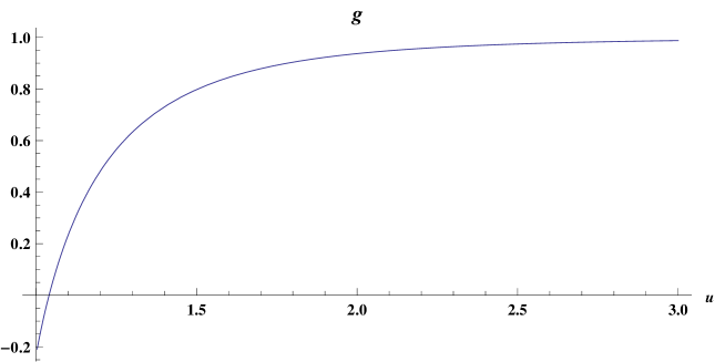
Figure 1: The blackhole factor $g$ as a function of $u\equiv r/\bar{r}_{h}$. We have plotted $g$ along the y-axis and $u$ along the x-axis. Using above considerations, one may trust the result for $u>1.02$.

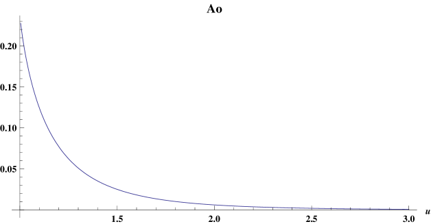
Figure 2: Non-extremal contribution to the warp factor given by $A_{0}$ plotted as a function of $u\equiv r/\bar{r}_{h}$. $A_{0}$ is plotted along y-axis, and $u$ is still along the x-axis and our analysis is valid for $u>1.02$.

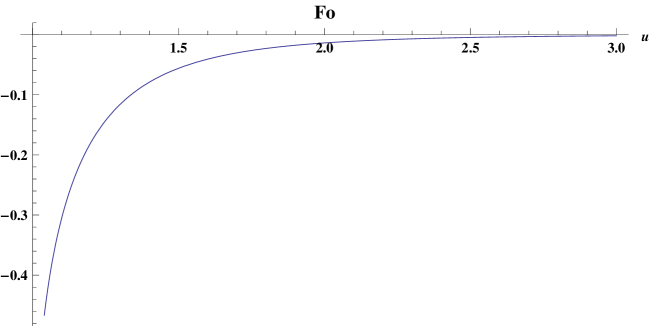
Figure 3: The squashing factor given by the resolution function $F_{0}$ as a function of $u\equiv r/\bar{r}_{h}$. Note that $F_{0}$ is always negative for all distances outside the black hole horizon. We plot $F_{0}$ along the y-axis, and $u$ is along x-axis, as before with validity from $u>1.02$.

Finally, note that the identification of $F$ with $a^{2}$ in (2) implies that the resolution parameter is given by

$$a^{2}= a_{0}^{2}+\frac{5g_{s}M^{2}p_{11}r_{h}^{2}}{32\pi N}+\frac{g_{s}M^{2}}{N}\frac{r_{h}^{2}}{4\pi}\left[p_{12}{\rm log}~{}r+p_{13}{\rm log}^{2}r\right]$$ (63)

$$+{1\over 4\pi}\left({g_{s}M^{2}\over N}\right)\left(g_{s}N_{f}\right)r_{h}^{4}\left(p_{14}{{\rm log}~{}r\over r^{2}}+{p_{15}\over r^{2}}\right){\rm log}\left(\rm{sin}\frac{\theta_{1}}{2}\rm{sin}\frac{\theta_{2}}{2}\right)$$

where we show the bare resolution parameter in $F$ and $a^{2}$. The coefficients $p_{ij}$ are constant numbers that could be determined from (2.1.2) and Appendix C. The above representation of the resolution parameter is perfectly consistent with our conjecture in [6]: the resolution parameter will pick up dependence on the horizon radius $r_{h}$. Interestingly we now have managed to get the leading order ${g_{s}M^{2}\over N}{\rm log}~{}r$ corrections to the result.

However there is one issue that might be confusing the reader. From Figure 3 we see that $F_{0}$ is always negative for all values of $r$ in the range $r_{h}\leq r<\infty$. Our identification of $F$ with $a^{2}$ would then imply $a$ to be a purely imaginary number. However surprisingly this does not create a problem. As we will show in the next subsection, all the fluxes etc. are completely expressed in terms of $a^{2}$, so that $a$ does not appear anywhere. Even terms with logarithms, for example (2.3), appear as ${\rm log}~{}|a^{2}|$, so that $a^{2}<0$ do not create any inconsistencies. This is of course shouldn’t come as a surprise because the resolution parameter appear in the metric (2) as $1+F_{0}$ and since $|F_{0}|<1$ it shouldn’t lead to any inconsistencies no matter how we relate $F_{0}$ to $a$.

In our opinion the result that we presented above is probably the first time where the backreaction effects from black hole, including the resolution factor, are taken into account in a self-consistent way to lowest orders in $g_{s}N_{f}$ and $g_{s}M^{2}/N$. To this order, as we showed above, the backreactions from fluxes and branes could be consistently ignored in the near horizon limit (41). One may now take this background and compute the IR effects for large $N$ thermal QCD. However before we go about studying these effects we would like to dwell, just for the sake of completeness, on the corrections to the Klebanov-Strassler three-form fluxes that arise from the backreactions of the black-hole, local brane sources, and the resolution parameter. Readers wishing to know our results may however skip the next sub-section altogether and proceed on with the calculations of the RG flows and the effects of the chemical potential.

2.2 The three-form fluxes revisited

In the above subsection we managed to provide a detailed derivation of the non-extremal limit of the Klebanov-Strassler type solution with a background warped resolved conifold. The ansatze that we used to solve for the fluxes was (49) where we divided the three-form fluxes into two pieces: one coming from the known Ouyang fluxes, and the other coming from the various backreactions. The second piece, for both RR and NS three-form fluxes, received contributions from the bare resolution parameter $a_{0}^{2}$ and the $g_{s}M^{2}/N$ terms in addition to the ${\cal O}(r_{h})$ terms. In the following we will not only justify this but also provide the form of the three-form fluxes including the above-mentioned corrections in the limit where the second squashing factor ${\cal G}$ in (2) is negligible. Our analysis will also not be affected by the constraint (41) that we had to impose to solve EOMs in the above subsection. In particular this means that the radial coordinate may take all values above $r_{h}$.

Using the metric (10) and (2) with the condition (2), the non-ISD RR three-form flux $\widetilde{F}_{3}\equiv F_{3}-C_{0}H_{3}$ takes the following form:

$${\widetilde{F}}_{3}=\left(\widetilde{a}_{o}-{3\over 2\pi r^{g_{s}N_{f}}}\right)\sum_{\alpha}{2M(r)c_{\alpha}\over r^{\epsilon_{(\alpha)}}}\left({\rm sin}~{}\theta_{1}~{}d\theta_{1}\wedge d\phi_{1}-\sum_{\alpha}{f_{\alpha}\over r^{\gamma_{(\alpha)}}}~{}{\rm sin}~{}\theta_{2}~{}d\theta_{2}\wedge d\phi_{2}\right)$$

$$~{}~{}\wedge~{}{e_{\psi}\over 2}-\sum_{\alpha}{3g_{s}M(r)N_{f}d_{\alpha}\over 4\pi r^{\sigma_{(\alpha)}}}~{}{dr}\wedge e_{\psi}\wedge\left({\rm cot}~{}{\theta_{2}\over 2}~{}{\rm sin}~{}\theta_{2}~{}d\phi_{2}-\sum_{\alpha}{g_{\alpha}\over r^{\rho_{(\alpha)}}}~{}{\rm cot}~{}{\theta_{1}\over 2}~{}{\rm sin}~{}\theta_{1}~{}d\phi_{1}\right)$$

$$-\sum_{\alpha}{3g_{s}M(r)N_{f}e_{\alpha}\over 8\pi r^{\tau_{(\alpha)}}}~{}{\rm sin}~{}\theta_{1}~{}{\rm sin}~{}\theta_{2}\left({\rm cot}~{}{\theta_{2}\over 2}~{}d\theta_{1}+\sum_{\alpha}{h_{\alpha}\over r^{\delta_{(\alpha)}}}~{}{\rm cot}~{}{\theta_{1}\over 2}~{}d\theta_{2}\right)\wedge d\phi_{1}\wedge d\phi_{2}$$ (64)

with $\widetilde{a}_{o}=1+{3\over 2\pi}$ and is defined in the intermediate region $r_{\rm min}<r<r_{o}$. The additional contributions to (64) are all proportional to powers of $r_{h}$, as they vanish in the ISD case. Finally, the quantity $\epsilon_{(\alpha)}$ is defined in the following way:

$$\epsilon_{(\alpha)}~{}=~{}\alpha+\sum_{n}{b_{\alpha n}\over r^{n}}$$ (65)

with $b_{\alpha n}$ are functions of $g_{s}N_{f},M$ and the horizon radius $r_{h}$. In a similar fashion $\rho_{(\alpha)},\sigma_{(\alpha)},\delta_{(\alpha)}$ etc are also defined. The other coefficients, for example $c_{\alpha},...h_{\alpha}$ would again be functions of $g_{s}N_{f}$ and $r_{h}$, but also of the resolution factor $a$ (including the internal angular coordinates). The resolution factor appears from the gravity dual that we considered in [6] i.e a resolved warped deformed confold with the resolution factor can be viewed as a function dependent on the horizon radius $r_{h}$. We will argue this in details below. The coefficients $b_{\alpha n}$ can be represented in terms of the following matrix:

$$b_{\{\alpha n\}}~{}\equiv~{}\begin{pmatrix}b_{00}&~{}b_{01}&~{}b_{02}&~{}b_{03}&....\\ b_{10}&~{}b_{11}&~{}b_{12}&~{}b_{13}&....\\ b_{20}&~{}b_{21}&~{}b_{22}&~{}b_{23}&....\\ b_{30}&~{}b_{31}&~{}b_{32}&~{}b_{33}&....\\ ...&...&...&...&....\\ b_{m0}&~{}b_{m1}&~{}b_{m2}&~{}b_{m3}&....\end{pmatrix}$$ (66)

The elements of the matrix $b_{\alpha n}$ can be determined in terms of the $c_{0},c_{1},c_{2},..$ coefficients that appears in the expansion ${c_{\alpha}\over r^{\epsilon_{(\alpha)}}}$. This is one reason of writing the various powers of $r$ using different symbols. For example $\sigma_{(\alpha)}$ will have a similar expansion as (65) but with a different matrix. The various elements of the matrix will now be determined in terms of $d_{0},d_{1},d_{2},..$ etc as one would expect. For the first case, we have managed to determine $c_{\alpha}$ up to few terms. They are represented as:

$$c_{0}~{}=~{}1+{\cal O}(r_{h}),~{}~{}~{}c_{1}~{}=~{}{\cal O}(r_{h}),~{}~{}~{}c_{2}~{}=~{}{9a^{2}g_{s}N_{f}\over 2\pi\zeta^{2}}\left(1-{3\over 2}{\rm log}~{}\zeta\right)+{\cal O}(r_{h})$$ (67)

where $a$ is the resolution factor and $\zeta$ is a parameter whose importance will become apparent soon. Once we know $c_{\alpha}$, it is not too difficult to get the relations between the various components of the matrix (66). One may now show that the components $b_{\alpha n}$ satisfy:

$$b_{00}~{}=~{}b_{01}~{}=~{}b_{10}~{}=~{}{\cal O}(r_{h})$$

$$c_{0}b_{02}~{}+~{}c_{1}b_{11}~{}+~{}c_{2}b_{20}~{}=~{}-{27a^{2}g_{s}N_{f}\over 4\pi\zeta^{2}}~{}+{\cal O}(r_{h})$$

$$2c_{0}b_{00}b_{01}~{}+~{}c_{1}b_{10}~{}=~{}{\cal O}(r_{h})$$

$$c_{0}b^{2}_{01}~{}+~{}2c_{0}b_{00}b_{02}~{}+~{}2c_{1}b_{10}b_{11}~{}+~{}c_{2}b_{20}~{}=~{}{\cal O}(r_{h})$$ (68)

Following the above set of relations one may show that:

$$\sum_{\alpha}{c_{\alpha}\over r^{\epsilon_{(\alpha)}}}~{} = ~{}1+{9a^{2}g_{s}N_{f}\over 2\pi\zeta^{2}r^{2}}\left(1-{3\over 2}{\rm log}~{}\zeta\right)-{27a^{2}g_{s}N_{f}\over 4\pi\zeta^{2}}\cdot{{\rm log}~{}r\over r^{2}}+{{\cal O}(r_{h})\over r^{2}}+{\cal O}(r_{h})$$ (69)

$$\equiv ~{}1+{9g_{s}N_{f}\over 4\pi}\cdot{a^{2}(r_{h},g_{s}N_{f})\over(\zeta r)^{2}}\cdot\left[2-3{\rm log}~{}(\zeta r)\right]+{\cal O}(r_{h},g_{s}^{2}N_{f}^{2})$$

which is consistent with what we discussed in [6], namely, the resolution parameter $a$ can be thought of as a function of ($r_{h},M,g_{s}N_{f}$), including the radial and the angular directions, i.e

$$a^{2}~{}=~{}a^{2}(r_{h},M,g_{s}N_{f})~{}=~{}a^{2}_{0}+\sum_{\alpha=1}^{\infty}{b_{\alpha}g_{s}^{\alpha}[M(r)r_{h}]^{\alpha+1}\over N^{\alpha}r^{\epsilon_{(\alpha)}}}$$ (70)

with $b_{\alpha}$ being functions of the angular directions so that this is consistent with (63). These can be determined by comparing (70) with (63) derived in the previous subsection (note that (63) implies $b_{0}=0$). The other similar factors appearing in the flux (73) are given in terms of the following series expansions similar to (69) above:

$$\sum_{\alpha}{d_{\alpha}\over r^{\sigma_{(\alpha)}}}~{}=~{}1+{18a^{2}(r_{h},M,g_{s}N_{f}){\rm log}~{}(\zeta r)\over(\zeta r)^{2}}+{\cal O}(r_{h},M,g_{s}N_{f})$$

$$\sum_{\alpha}{e_{\alpha}\over r^{\tau_{(\alpha)}}}~{}=~{}1-{18a^{2}(r_{h},M,g_{s}N_{f}){\rm log}~{}(\zeta r)\over(\zeta r)^{2}}+{\cal O}(r_{h},M,g_{s}N_{f})$$ (71)

Note also that there are squashing factors given by ${f_{\alpha}\over r^{\gamma_{(\alpha)}}},{g_{\alpha}\over r^{\rho_{(\alpha)}}}$ and ${h_{\alpha}\over r^{\delta_{(\alpha)}}}$. These squashing factors distort the spheres and therefore affect the fluxes on them. Its easy to show that these factors are given by:

$$\sum_{\alpha}{f_{\alpha}\over r^{\gamma_{(\alpha)}}}~{} = ~{}1-{729\over 32\pi^{2}}\cdot{g_{s}^{2}N_{f}^{2}a^{4}(r_{h},M,g_{s}N_{f})\over(\zeta r)^{4}}\cdot{\rm log}~{}(\zeta r)\left[2-3{\rm log}~{}(\zeta r)\right]+{\cal O}(r_{h},M,g_{s}^{2}N_{f}^{2})$$

$$+{81\over 8\pi}\cdot{g_{s}N_{f}a^{2}(r_{h},M,g_{s}N_{f}){\rm log}~{}(\zeta r)\over(\zeta r)^{2}}$$

$$= ~{}1+{81\over 2}\cdot{g_{s}N_{f}a^{2}(r_{h},M,g_{s}N_{f}){\rm log}~{}(\zeta r)\over 4\pi r^{2}+9g_{s}N_{f}a^{2}(r_{h},M,g_{s}N_{f})[2-3~{}{\rm log}~{}(\zeta r)]}+{\cal O}(r_{h},M,g_{s}^{2}N_{f}^{2})$$

$$\sum_{\alpha}{g_{\alpha}\over r^{\rho_{(\alpha)}}}~{} = ~{}1+{36a^{2}(r_{h},M,g_{s}N_{f}){\rm log}~{}(\zeta r)\over(\zeta r)^{3}}-{648a^{4}(r_{h},M,g_{s}N_{f}){\rm log}^{2}(\zeta r)\over(\zeta r)^{5}}+{\cal O}(r_{h},M,g_{s}^{2}N_{f}^{2})$$

$$= ~{}1+{36a^{2}(r_{h},M,g_{s}N_{f})~{}{\rm log}~{}(\zeta r)\over(\zeta r)^{3}+18a^{2}(r_{h},M,g_{s}N_{f})\zeta r~{}{\rm log}~{}(\zeta r)}+{\cal O}(r_{h},M,g_{s}^{2}N_{f}^{2})$$

$$\sum_{\alpha}{h_{\alpha}\over r^{\delta_{(\alpha)}}}~{} = ~{}1+{36a^{2}(r_{h},M,g_{s}N_{f}){\rm log}~{}(\zeta r)\over(\zeta r)^{2}}+{648a^{4}(r_{h},M,g_{s}N_{f}){\rm log}^{2}(\zeta r)\over(\zeta r)^{4}}+{\cal O}(r_{h},M,g_{s}^{2}N_{f}^{2})$$

$$= ~{}1+{36a^{2}(r_{h},M,g_{s}N_{f})~{}{\rm log}~{}(\zeta r)\over(\zeta r)^{2}+18a^{2}(r_{h},M,g_{s}N_{f})~{}{\rm log}~{}(\zeta r)}+{\cal O}(r_{h},M,g_{s}^{2}N_{f}^{2})$$

The far IR physics is then determined from (73) and the squashing factors (2.2) by making the replacement $(\zeta r)~{}\to r$ to the radial coordinate. Note also that all the flux components are expressed in terms of $a^{2}$ and therefore the sign of $a^{2}$ can be directly inserted here. Considering all the above, this then gives us exactly the result that we had in [6], namely:

$${\widetilde{F}}_{3} = 2M{\bf A_{1}}\left(1+{3g_{s}N_{f}\over 2\pi}~{}{\rm log}~{}r\right)~{}e_{\psi}\wedge\frac{1}{2}\left({\rm sin}~{}\theta_{1}~{}d\theta_{1}\wedge d\phi_{1}-{\bf B_{1}}~{}{\rm sin}~{}\theta_{2}~{}d\theta_{2}\wedge d\phi_{2}\right)$$ (73)

$$-{3g_{s}MN_{f}\over 4\pi}{\bf A_{2}}~{}{dr\over r}\wedge e_{\psi}\wedge\left({\rm cot}~{}{\theta_{2}\over 2}~{}{\rm sin}~{}\theta_{2}~{}d\phi_{2}-{\bf B_{2}}~{}{\rm cot}~{}{\theta_{1}\over 2}~{}{\rm sin}~{}\theta_{1}~{}d\phi_{1}\right)$$

$$-{3g_{s}MN_{f}\over 8\pi}{\bf A_{3}}~{}{\rm sin}~{}\theta_{1}~{}{\rm sin}~{}\theta_{2}\left({\rm cot}~{}{\theta_{2}\over 2}~{}d\theta_{1}+{\bf B_{3}}~{}{\rm cot}~{}{\theta_{1}\over 2}~{}d\theta_{2}\right)\wedge d\phi_{1}\wedge d\phi_{2}$$

where we have taken $M(r)~{}\to~{}M$ in the far IR, and the various coefficients ${\bf A}_{i},{\bf B}_{i}$ are related to (69) and (2.2) as:

$$\sum_{\alpha}{c_{\alpha}\over r^{\epsilon_{(\alpha)}}}~{}\equiv~{}{\bf A}_{1},~{}~{}~{}\sum_{\alpha}{d_{\alpha}\over r^{\sigma_{(\alpha)}}}~{}\equiv~{}{\bf A}_{2},~{}~{}~{}\sum_{\alpha}{e_{\alpha}\over r^{\tau_{(\alpha)}}}~{}\equiv~{}{\bf A}_{3}$$

$$\sum_{\alpha}{f_{\alpha}\over r^{\gamma_{(\alpha)}}}~{}\equiv~{}{\bf B}_{1},~{}~{}~{}\sum_{\alpha}{g_{\alpha}\over r^{\rho_{(\alpha)}}}~{}\equiv~{}{\bf B}_{2},~{}~{}~{}\sum_{\alpha}{h_{\alpha}\over r^{\delta_{(\alpha)}}}~{}\equiv~{}{\bf B}_{3}$$ (74)

As we mentioned before, the additional contributions to (2.2) are all proportional to powers of $r_{h}$, as they vanish in the ISD case. Needless to say, the functional form for $F_{3}$ is consistent with (49).

The NS three-form flux $H_{3}$ is now more interesting. Unlike $\widetilde{F}_{3}$, it has to be closed. When the resolution parameter $a$ and $M$ are just constants, it is easy to construct a closed $H_{3}$. In the presence of non-constant $a$ and $M(r)$, finding a closed $H_{3}$ is more non-trivial. For our case $H_{3}$ is given by:

$$H_{3}=\sum_{\alpha}{6g_{s}M(r)k_{\alpha}\over r^{\beta_{(\alpha)}}}\Bigg{[}1+\frac{1}{2\pi}-\frac{\left({\rm cosec}~{}\frac{\theta_{1}}{2}~{}{\rm cosec}~{}\frac{\theta_{2}}{2}\right)^{g_{s}N_{f}}}{2\pi r^{{9g_{s}N_{f}\over 2}}}\Bigg{]}~{}\left[dr+\sum_{i}{\cal O}(r_{h})d\sigma_{i}\right]$$

$$\wedge\frac{1}{2}\Bigg{(}{\rm sin}~{}\theta_{1}~{}d\theta_{1}\wedge d\phi_{1}-\sum_{\alpha}{p_{\alpha}\over r^{\kappa_{(\alpha)}}}~{}{\rm sin}~{}\theta_{2}~{}d\theta_{2}\wedge d\phi_{2}\Bigg{)}+\sum_{\alpha}\frac{3g^{2}_{s}M(r)N_{f}l_{\alpha}}{8\pi r^{\theta_{(\alpha)}}}\Bigg{(}\frac{dr}{r}\wedge e_{\psi}-\frac{1}{2}de_{\psi}\Bigg{)}$$

$$\wedge\Bigg{(}{\rm cot}~{}\frac{\theta_{2}}{2}~{}d\theta_{2}-\sum_{\alpha}{q_{\alpha}\over r^{\xi_{(\alpha)}}}~{}{\rm cot}~{}\frac{\theta_{1}}{2}~{}d\theta_{1}\Bigg{)}+g_{s}{dM(r)\over dr}\left(b_{1}(r)\cot\frac{\theta_{1}}{2}\,d\theta_{1}+b_{2}(r)\cot\frac{\theta_{2}}{2}\,d\theta_{2}\right)$$

$$\wedge e_{\psi}\wedge dr+{3g_{s}\over 4\pi}{dM(r)\over dr}\left(1+g_{s}N_{f}-{1\over r^{2g_{s}N_{f}}}+{9a^{2}g_{s}N_{f}\over r^{2}}+b_{3}(r)\right)\log\left(\sin\frac{\theta_{1}}{2}\sin\frac{\theta_{2}}{2}\right)$$

$$\sin\theta_{1}\,d\theta_{1}\wedge d\phi_{1}\wedge dr-{g_{s}\over 12\pi}{dM(r)\over dr}\Bigg{(}2-{27a^{2}g_{s}N_{f}\over r^{2}}+9g_{s}N_{f}-{1\over r^{16g_{s}N_{f}}}-{1\over r^{2g_{s}N_{f}}}\Bigg{)}$$

$$\log\left(\sin\frac{\theta_{1}}{2}\sin\frac{\theta_{2}}{2}\right)\sin\theta_{2}\,d\theta_{2}\wedge d\phi_{2}\wedge dr-{g_{s}b_{4}(r)\over 12\pi}{dM(r)\over dr}~{}\log\left(\sin\frac{\theta_{1}}{2}\sin\frac{\theta_{2}}{2}\right)\sin\theta_{2}\,d\theta_{2}\wedge d\phi_{2}\wedge dr$$

(75)

with ($k_{\alpha},...,q_{\alpha}$) being constants, $\sigma_{i}\equiv(\theta_{i},\phi_{i})$ and $b_{n}=\sum_{m}{a_{nm}\over r^{m+\widetilde{\epsilon}_{m}}}$ where $a_{nm}\equiv a_{nm}(g_{s}N_{f},M,r_{h})$ and $\widetilde{\epsilon}_{m}\equiv\widetilde{\epsilon}_{m}(g_{s}N_{f},M,r_{h})$.

Note that in addition to the simplest ${\cal O}(r_{h})$ term that we mentioned above, there would be more terms of the same order that vanish in the ISD limit. We might also wonder about terms of the form $da/dr$ and $da/d\sigma_{i}$. From the form of (70) we see that these terms themselves are of ${\cal O}(M)$ so to this order they could either be absorbed in $dM(r)/dr$ terms or in the ${\cal O}(r_{h})$ terms. The various squashing factor etc are now given by:

$$\sum_{\alpha}{k_{\alpha}\over r^{\beta_{(\alpha)}}}~{} = 1-{3a^{2}(r_{h},M,g_{s}N_{f})\over(\zeta r)^{2}}+{\cal O}(r_{h},M,g^{2}_{s}N^{2}_{f})$$

$$\sum_{\alpha}{l_{\alpha}\over r^{\theta_{(\alpha)}}}~{} = 1+{36a^{2}(r_{h},M,g_{s}N_{f})~{}{\rm log}~{}(\zeta r)\over\zeta r}+{\cal O}(r_{h},M,g^{2}_{s}N^{2}_{f})$$

$$\sum_{\alpha}{p_{\alpha}\over r^{\kappa_{(\alpha)}}}~{} = 1+{3g_{s}a^{2}(r_{h},M,g_{s}N_{f})\over(\zeta r)^{2}}+{9g_{s}a^{4}(r_{h},M,g_{s}N_{f})\over(\zeta r)^{4}}+{\cal O}(r_{h},M,g^{2}_{s}N^{2}_{f})$$

$$= 1+{3g_{s}a^{2}(r_{h},M,g_{s}N_{f})\over(\zeta r)^{2}-3a^{2}(r_{h},M,g_{s}N_{f})}+{\cal O}(r_{h},M,g_{s}^{2}N_{f}^{2})$$

$$\sum_{\alpha}{q_{\alpha}\over r^{\xi_{(\alpha)}}}~{} = 1+{72a^{2}(r_{h},M,g_{s}N_{f})~{}{\rm log}~{}(\zeta r)\over\zeta r}-{2592a^{4}(r_{h},M,g_{s}N_{f})~{}{\rm log}^{2}~{}(\zeta r)\over(\zeta r)^{2}}+{\cal O}(r_{h},M,g^{2}_{s}N^{2}_{f})$$ (76)

$$= 1+{72a^{2}(r_{h},M,g_{s}N_{f})~{}{\rm log}~{}(\zeta r)\over\zeta r+36a^{2}(r_{h},M,g_{s}N_{f})~{}{\rm log}~{}(\zeta r)}+{\cal O}(r_{h},M,g_{s}^{2}N_{f}^{2})$$

To study the far IR physics, we again consider $M(r)\to M$, with the various expansions in (2.2) are related to ${\bf A_{4},A_{5},B_{4}}$ and ${\bf B_{5}}$ respectively. Note again that the resolution parameter in all the coefficients appear as $a^{2}$. This then reproduces again the far IR result of [25] as well as the expected ansatze (49), namely:

$$H_{3} = {6g_{s}{\bf A_{4}}M}\Bigg{(}1+\frac{9g_{s}N_{f}}{4\pi}~{}{\rm log}~{}r+\frac{g_{s}N_{f}}{2\pi}~{}{\rm log}~{}{\rm sin}\frac{\theta_{1}}{2}~{}{\rm sin}\frac{\theta_{2}}{2}\Bigg{)}\frac{dr}{r}$$ (77)

$$\wedge\frac{1}{2}\Bigg{(}{\rm sin}~{}\theta_{1}~{}d\theta_{1}\wedge d\phi_{1}-{\bf B_{4}}~{}{\rm sin}~{}\theta_{2}~{}d\theta_{2}\wedge d\phi_{2}\Bigg{)}+\frac{3g^{2}_{s}MN_{f}}{8\pi}{\bf A_{5}}\Bigg{(}\frac{dr}{r}\wedge e_{\psi}-\frac{1}{2}de_{\psi}\Bigg{)}$$

$$\hskip 42.67912pt\wedge\Bigg{(}{\rm cot}~{}\frac{\theta_{2}}{2}~{}d\theta_{2}-{\bf B_{5}}~{}{\rm cot}~{}\frac{\theta_{1}}{2}~{}d\theta_{1}\Bigg{)}$$

with the necessary ${\cal O}(r_{h})$ terms that vanish when the horizon radius vanishes.

In the far IR the closure of $H_{3}$ is again non-trivial because the resolution parameter $a$ is no longer a constant now, although $M(r)\to M$. All the informations of non-constant $a$ are captured in the coefficients ${\bf A_{4,5}}$ and the squashing factors ${\bf B_{4,5}}$. In the following section we will determine the resolution parameter to ${\cal O}(M^{2})$ in the IR. This means up to this order, the closure of $H_{3}$ implies the following three conditions:

$$(i)~{}~{}\alpha_{2}{\rm cot}~{}{\theta_{2}\over 2}~{}{\partial{\bf A_{5}}\over\partial\theta_{1}}+\alpha_{2}~{}{\bf A_{5}}{\rm cot}~{}{\theta_{1}\over 2}~{}{\partial{\bf B_{5}}\over\partial\theta_{1}}+{\cal O}(r_{h},M^{3},g_{s}N_{f})=0$$ (78)

$$(ii)~{}~{}\alpha_{1}{\rm sin}~{}{\theta_{1}}~{}{\partial{\bf A_{4}}\over\partial\theta_{2}}+\alpha_{2}{\rm cos}~{}{\theta_{1}}~{}{\rm cot}~{}{\theta_{2}\over 2}~{}{\partial{\bf A_{5}}\over\partial\theta_{1}}-\alpha_{3}{\rm sin}~{}{\theta_{1}}~{}{\rm cot}~{}{\theta_{2}\over 2}~{}{\partial{\bf A_{5}}\over\partial r}$$

$$~{}~{}~{}~{}~{}~{}~{}~{}~{}~{}~{}~{}~{}~{}~{}+\alpha_{2}{\bf A_{5}}{\rm cos}~{}{\theta_{1}}~{}{\rm cot}~{}{\theta_{1}\over 2}~{}{\partial{\bf B_{5}}\over\partial\theta_{2}}+{\cal O}(r_{h},M^{3},g_{s}N_{f})=0$$

$$(iii)~{}~{}\alpha_{1}~{}{\bf B_{4}}~{}{\rm sin}~{}{\theta_{2}}~{}{\rm cot}~{}{\theta_{1}\over 2}~{}{\partial{\bf A_{4}}\over\partial\theta_{1}}-\alpha_{1}~{}{\bf A_{4}}~{}{\rm sin}~{}{\theta_{2}}~{}{\partial{\bf B_{4}}\over\partial\theta_{1}}-\alpha_{2}~{}{\bf A_{5}}~{}{\rm cos}~{}{\theta_{2}}~{}{\rm cot}~{}{\theta_{1}\over 2}~{}{\partial{\bf B_{5}}\over\partial\theta_{2}}$$

$$~{}~{}~{}~{}~{}~{}~{}~{}~{}~{}~{}~{}~{}~{}~{}-\alpha_{3}~{}{\bf A_{5}}~{}{\rm sin}~{}{\theta_{2}}~{}{\rm cot}~{}{\theta_{1}\over 2}~{}{\partial{\bf B_{5}}\over\partial r}+\alpha_{2}~{}{\rm cos}~{}{\theta_{2}}~{}{\rm cot}~{}{\theta_{2}\over 2}~{}{\partial{\bf A_{5}}\over\partial\theta_{1}}$$

$$~{}~{}~{}~{}~{}~{}~{}~{}~{}~{}~{}~{}~{}~{}~{}~{}-\alpha_{3}~{}{\bf B_{5}}~{}{\rm sin}~{}{\theta_{2}}~{}{\rm cot}~{}{\theta_{1}\over 2}~{}{\partial{\bf A_{5}}\over\partial r}+{\cal O}(r_{h},M^{3},g_{s}N_{f})=0$$

where $\alpha_{1},\alpha_{2}$ and $\alpha_{3}$ are defined as:

$$\alpha_{1}={3g_{s}M\over 2}\Bigg{(}1+\frac{9g_{s}N_{f}}{4\pi}~{}{\rm log}~{}r+\frac{g_{s}N_{f}}{2\pi}~{}{\rm log}~{}{\rm sin}\frac{\theta_{1}}{2}~{}{\rm sin}\frac{\theta_{2}}{2}\Bigg{)}$$

$$\alpha_{2}={3g_{s}^{2}MN_{f}\over 8\pi r},~{}~{}~{}~{}~{}~{}~{}~{}\alpha_{3}=-{3g_{s}^{2}MN_{f}\over 16\pi}=-{r\alpha_{2}\over 2}$$ (79)

The RR three-form flux ${\widetilde{F}}_{3}\equiv F_{3}-C_{0}H_{3}$ is not closed, but it satisfies the condition $d{\widetilde{F}}_{3}=-dC_{0}\wedge H_{3}$, which is equivalent to the statement that $F_{3}$ is closed. Of course as described in [25], the closure of $F_{3}$ is only in Region 1. In Region 2 there are anti five-brane sources that make $F_{3}$ non-closed. The closure of $F_{3}$ in Region 1 implies the following nine conditions on the various coefficients of the three-form fluxes:

$$(iv)~{}~{}\beta_{1}{\partial{\bf A_{1}}\over\partial r}~{}{\rm sin}~{}\theta_{1}-\beta_{2}~{}{\partial{\bf A_{2}}\over\partial\theta_{1}}~{}{\rm cot}~{}{\theta_{1}\over 2}~{}{\rm sin}~{}\theta_{1}-\beta_{2}~{}{\bf A_{2}}~{}{\partial{\bf B_{2}}\over\partial\theta_{1}}~{}{\rm cot}~{}{\theta_{1}\over 2}~{}{\rm sin}~{}\theta_{1}$$

$$+k\alpha_{1}~{}{\bf A_{4}}~{}{\rm sin}~{}\theta_{1}+k\alpha_{2}~{}{\bf A_{5}}~{}{{\bf B_{5}}}~{}{\rm cot}~{}{\theta_{1}\over 2}~{}{\rm cos}~{}\theta_{1}+k\alpha_{2}~{}{\bf A_{5}}~{}{{\bf B_{5}}}~{}{\rm cot}~{}{\theta_{1}\over 2}+{\cal O}(r_{h},M^{3},g_{s}N_{f})=0$$

$$(v)~{}~{}-\beta_{1}~{}{\bf B_{1}}~{}{\partial{\bf A_{1}}\over\partial r}~{}{\rm sin}~{}\theta_{2}+\beta_{1}~{}{\bf A_{1}}~{}{\partial{\bf B_{1}}\over\partial r}~{}{\rm sin}~{}\theta_{2}+\beta_{2}~{}{\partial{\bf A_{2}}\over\partial\theta_{2}}~{}{\rm cot}~{}{\theta_{2}\over 2}~{}{\rm sin}~{}\theta_{2}$$

$$-k\alpha_{1}~{}{\bf A_{4}}~{}{\bf B_{4}}~{}{\rm sin}~{}\theta_{2}-k\alpha_{2}~{}{\bf A_{5}}~{}{\rm cot}~{}{\theta_{2}\over 2}~{}{\rm cos}~{}\theta_{2}+k\alpha_{2}~{}{\bf A_{5}}~{}{\rm cot}~{}{\theta_{2}\over 2}+{\cal O}(r_{h},M^{3},g_{s}N_{f})=0$$

$$(vi)~{}~{}\beta_{1}~{}{\partial{\bf B_{2}}\over\partial r}~{}{\rm cos}~{}{\theta_{2}}~{}{\rm sin}~{}\theta_{1}-\beta_{2}~{}{\partial{\bf A_{2}}\over\partial\theta_{1}}~{}{\rm cot}~{}{\theta_{2}\over 2}~{}{\rm sin}~{}\theta_{1}~{}{\rm cos}~{}\theta_{1}+\beta_{2}~{}{\bf B_{2}}~{}{\partial{\bf A_{2}}\over\partial\theta_{1}}~{}{\rm cot}~{}{\theta_{1}\over 2}~{}{\rm sin}~{}\theta_{1}~{}{\rm cos}~{}\theta_{2}$$

$$-\beta_{2}~{}{\bf A_{2}}~{}{\partial{\bf B_{2}}\over\partial\theta_{1}}~{}{\rm cot}~{}{\theta_{1}\over 2}~{}{\rm sin}~{}\theta_{1}~{}{\rm cos}~{}\theta_{2}+\beta_{3}~{}{\partial{\bf A_{3}}\over\partial r}~{}{\rm cot}~{}{\theta_{2}\over 2}-k\alpha_{1}~{}{\bf A_{4}}~{}{\rm sin}~{}\theta_{1}$$

$$~{}~{}~{}~{}~{}~{}-k\alpha_{2}~{}{\bf A_{5}}~{}{\bf B_{5}}~{}{\rm cot}~{}{\theta_{1}\over 2}~{}{\rm cos}~{}\theta_{1}+k\alpha_{2}~{}{\bf A_{5}}~{}{\bf B_{5}}~{}{\rm cot}~{}{\theta_{1}\over 2}~{}{\rm cos}~{}\theta_{2}+{\cal O}(r_{h},M^{3},g_{s}N_{f})=0$$

$$(vii)~{}~{}-\beta_{1}~{}{\bf B_{1}}~{}{\partial{\bf A_{1}}\over\partial r}~{}{\rm sin}~{}\theta_{2}~{}{\rm cos}~{}\theta_{1}-\beta_{1}~{}{\bf A_{1}}~{}{\partial{\bf B_{1}}\over\partial r}~{}{\rm sin}~{}\theta_{2}~{}{\rm cos}~{}\theta_{1}-\beta_{2}~{}{\partial{\bf A_{2}}\over\partial\theta_{2}}~{}{\rm cot}~{}{\theta_{2}\over 2}~{}{\rm sin}~{}\theta_{2}~{}{\rm cos}~{}\theta_{1}$$

$$-\beta_{2}~{}{\bf B_{2}}~{}{\partial{\bf A_{2}}\over\partial\theta_{2}}~{}{\rm cot}~{}{\theta_{1}\over 2}~{}{\rm sin}~{}\theta_{1}~{}{\rm cos}~{}\theta_{2}-\beta_{2}~{}{\bf A_{2}}~{}{\partial{\bf B_{2}}\over\partial\theta_{2}}~{}{\rm cot}~{}{\theta_{1}\over 2}~{}{\rm sin}~{}\theta_{1}~{}{\rm cos}~{}\theta_{2}+\beta_{3}~{}{\bf B_{3}}~{}{\partial{\bf A_{3}}\over\partial r}~{}{\rm cot}~{}{\theta_{1}\over 2}$$

$$~{}~{}~{}~{}~{}~{}~{}~{}+\beta_{3}~{}{\bf A_{3}}~{}{\partial{\bf B_{3}}\over\partial r}~{}{\rm cot}~{}{\theta_{1}\over 2}+k\alpha_{2}~{}{\bf A_{5}}~{}{\rm cos}~{}\theta_{1}~{}{\rm cot}~{}{\theta_{2}\over 2}-k\alpha_{1}~{}{\bf A_{4}}~{}{\bf B_{4}}~{}{\rm sin}~{}\theta_{2}$$

$$~{}~{}~{}~{}~{}~{}~{}~{}~{}~{}~{}~{}~{}~{}~{}~{}~{}~{}~{}-k\alpha_{2}~{}{\bf A_{5}}~{}{\rm cot}~{}{\theta_{2}\over 2}~{}{\rm cos}~{}\theta_{2}+{\cal O}(r_{h},M^{3},g_{s}N_{f})=0$$

$$(viii)~{}~{}\beta_{1}~{}{\partial{\bf A_{1}}\over\partial\theta_{2}}~{}{\rm cos}~{}\theta_{2}+\beta_{1}~{}{\bf A_{1}}~{}{\partial{\bf B_{1}}\over\partial\theta_{1}}~{}{\rm sin}~{}\theta_{2}~{}{\rm cos}~{}\theta_{1}-\beta_{3}~{}{\bf B_{3}}~{}{\partial{\bf A_{3}}\over\partial\theta_{1}}~{}{\rm cot}~{}{\theta_{1}\over 2}+\beta_{3}~{}{\partial{\bf A_{3}}\over\partial\theta_{2}}~{}{\rm cot}~{}{\theta_{2}\over 2}$$

$$-\beta_{3}~{}{\bf A_{3}}~{}{\partial{\bf B_{3}}\over\partial\theta_{1}}~{}{\rm cot}~{}{\theta_{1}\over 2}-k\alpha_{3}~{}{\bf A_{5}}~{}{\rm cot}~{}{\theta_{2}\over 2}~{}{\rm sin}~{}\theta_{1}+k\alpha_{3}~{}{\bf A_{5}}~{}{\bf B_{5}}~{}{\rm cot}~{}{\theta_{1}\over 2}~{}{\rm sin}~{}\theta_{2}+{\cal O}(r_{h},M^{3},g_{s}N_{f})=0$$

$$(ix)~{}~{}\beta_{1}~{}{\partial{\bf A_{1}}\over\partial\theta_{2}}~{}{\rm sin}~{}\theta_{1}+k\alpha_{3}~{}{\bf A_{5}}~{}{\rm cot}~{}{\theta_{2}\over 2}~{}{\rm sin}~{}\theta_{1}+{\cal O}(r_{h},M^{3},g_{s}N_{f})=0$$

$$(x)~{}~{}\beta_{1}~{}{\bf A_{1}}~{}{\partial{\bf B_{1}}\over\partial\theta_{1}}~{}{\rm sin}~{}\theta_{2}+k\alpha_{3}~{}{\bf A_{5}}~{}{\bf B_{5}}~{}{\rm cot}~{}{\theta_{1}\over 2}~{}{\rm sin}~{}\theta_{2}+{\cal O}(r_{h},M^{3},g_{s}N_{f})=0$$

$$(xi)~{}~{}-\beta_{2}~{}{\partial{\bf A_{2}}\over\partial\theta_{1}}~{}{\rm cot}~{}{\theta_{2}\over 2}~{}{\rm sin}~{}\theta_{2}-k\alpha_{2}~{}{\bf A_{5}}~{}{\bf B_{5}}~{}{\rm cot}~{}{\theta_{1}\over 2}~{}{\rm cos}~{}\theta_{2}+k\alpha_{2}~{}{\bf A_{5}}~{}{\bf B_{5}}~{}{\rm cot}~{}{\theta_{1}\over 2}$$

$$~{}~{}~{}~{}~{}~{}~{}~{}~{}~{}~{}~{}~{}~{}~{}~{}~{}~{}~{}~{}~{}~{}~{}~{}~{}~{}~{}~{}~{}~{}~{}~{}~{}~{}~{}~{}+{\cal O}(r_{h},M^{3},g_{s}N_{f})=0$$

$$(xii)~{}~{}-\beta_{2}~{}{\bf A_{2}}~{}{\partial{\bf B_{2}}\over\partial\theta_{2}}~{}{\rm cot}~{}{\theta_{1}\over 2}~{}{\rm sin}~{}\theta_{1}+\beta_{2}~{}{\partial{\bf A_{2}}\over\partial\theta_{2}}~{}{\rm cot}~{}{\theta_{2}\over 2}~{}{\rm sin}~{}\theta_{2}-k\alpha_{2}~{}{\bf A_{5}}~{}{\rm cot}~{}{\theta_{2}\over 2}$$

$$~{}~{}~{}~{}~{}~{}~{}~{}~{}~{}~{}~{}~{}~{}~{}~{}~{}~{}-k\alpha_{2}~{}{\bf A_{5}}~{}{\rm cot}~{}{\theta_{2}\over 2}~{}{\rm cos}~{}\theta_{1}+{\cal O}(r_{h},M^{3},g_{s}N_{f})=0$$ (80)

where we have already defined $\alpha_{k},{\bf A_{n}}$ and ${\bf B_{m}}$. The $\beta_{i}$ are now defined as:

$$\beta_{1}=M\left(1+{3g_{s}N_{f}\over 2\pi}{\rm log}~{}r\right),~{}~{}~{}~{}~{}~{}\beta_{2}=-{3g_{s}MN_{f}\over 4\pi r}={2\beta_{3}\over r}$$ (81)

Note that in (78) and (2.2) we have separated the ${\cal O}(r_{h},M^{3},g_{s}N_{f})$ corrections from the resolution parameter $a^{2}$ in the fluxes. We may also absorb these corrections to the resolution parameter and write the three-form fluxes completely in terms of ${\cal O}(M^{3})$ corrections to the ${\cal O}(M)$ terms in the original Ouyang solution. This may also be interpreted as though every flux components sees a different resolution parameter $a_{k}^{2}$. Note also that we don’t have an ${\cal O}(M^{2})$ corrections to the Ouyang three-form fluxes. However from (70) we do expect an ${\cal O}(M)$ term for $a^{2}$, unless of course $b_{0}=0$ or $a_{0}$ is proportional to $M$. Comparing (70) with (55), (56) and (63) may imply $b_{0}=0$. Additionally, the scenario with $a^{2}_{0}$ being of ${\cal O}(M/N)$, is more likely, as in the absence of wrapped D5-branes the gauge theory is conformal with the gravity dual given by $AdS_{5}\times T^{1,1}$ [28]. Only in the presence of wrapped D5-branes the gravity dual becomes a resolved warped-deformed conifold so the resolution parameter $a_{0}$ should depend on $M$. This will be consistent with (55) and (2.1.2) as discussed earlier. In either case, it is clear that the fluxes that we take contribute the ${\cal O}(M^{3})$ terms to the original Ouyang fluxes. This helped us to get a consistent background in the presence of fluxes and a black-hole as we saw in the previous subsection. A more elaborate study will be delegated to [21].

Before we end this section, let us also see how the squashing factors in the three-form fluxes behave in the light of the result (63). To ${\cal O}(g_{s}M^{2}/N)$ the resolution parameter $a^{2}$ is only a function of the radial coordinate $r$. This means that ${\bf A_{n}},{\bf B_{m}}$ can be written as functions of $r$ to this order satisfying the closure conditions (78) and (2.2). For example, combining (63) and (78), ${\bf A_{5}}$ takes the following integral form:

$${\bf A_{5}}={1\over{\rm sin}~{}\theta_{1}~{}{\rm cot}~{}{\theta_{2}\over 2}}\int dr{a_{5}\over\alpha_{3}}$$ (82)

where $a_{5}$ is a function of the angular $\theta_{i}$ and the radial $r$ variable such that ${\partial{\bf A_{5}}\over\partial\theta_{i}}=0$. Similarly:

$${\bf B_{5}}={{\rm sin}~{}\theta_{1}~{}{\rm cot}~{}{\theta_{2}\over 2}\over{\rm sin}~{}\theta_{2}~{}{\rm cot}~{}{\theta_{1}\over 2}}~{}{\int dr~{}c_{5}\alpha_{3}^{-1}(r)\over\int dr^{\prime}~{}a_{5}\alpha_{3}^{-1}(r^{\prime})}$$ (83)

where again $c_{5}$ is like $a_{5}$ discussed above. Once ($a_{5},c_{5}$) are determined the two integral forms (82) and (83) not only satisfy the closure conditions (78) but also the necessary EOM. These two integral forms are also consistent with the conditions ($ix$) and ($x$) of (2.2) because $\alpha_{3}\equiv-{3g_{s}^{2}MN_{f}\over 16\pi}$ is a constant. Note however that, to this order, the integral form for (${\bf A_{4}},{\bf B_{4}}$) cannot be determined by this method, although we will know (${\bf A_{4}},{\bf B_{4}}$) in terms of the resolution parameter $a^{2}$ up to the ${\cal O}(r_{h},M^{3},g_{s}N_{f})$ corrections.

On the other hand both (${\bf A_{1}},{\bf B_{1}}$) do have an integral representation if we assume that (${\bf A_{4}},{\bf B_{4}}$) have some integral representation (which in turn will be determined in a different way from the one that we have followed here). If this is the case, then:

$${\bf A_{1}}=\int{dr\over\beta_{1}}~{}\left({a_{1}\over{\rm sin}~{}\theta_{1}}+k\alpha_{1}~{}{\bf A_{4}}+k\alpha_{2}~{}{\bf A_{5}}~{}{{\bf B_{5}}}~{}{\rm cot}~{}{\theta_{1}\over 2}~{}{\rm cot}~{}\theta_{1}+k\alpha_{2}~{}{\bf A_{5}}~{}{{\bf B_{5}}}~{}{\rm csc}^{2}~{}{\theta_{1}\over 2}\right)$$

$${\bf B_{1}}={\bf A_{1}}\int{dr\over\beta_{1}{\bf A_{1}}^{2}}~{}\left({b_{1}\over{\rm sin}~{}\theta_{2}}+k\alpha_{1}~{}{\bf A_{4}}~{}{\bf B_{4}}+k\alpha_{2}~{}{\bf A_{5}}~{}{\rm cot}~{}{\theta_{2}\over 2}~{}{\rm cot}~{}\theta_{2}-k\alpha_{2}~{}{\bf A_{5}}~{}{\rm csc}^{2}~{}{\theta_{2}\over 2}\right)$$

where ($a_{1},b_{1}$) are functions of $r$ and $\theta_{i}$ such that ${\partial{\bf A_{1}}\over\partial\theta_{i}}={\partial{\bf B_{1}}\over\partial\theta_{i}}=0$ in the same sense as mentioned earlier for the other cases. The other squashing factors in (2.2) do not however have such simpler integral forms.

Another interesting thing to note is that from condition ($xii$) of (2.2) we might get a simpler form for ${\bf A_{5}}$, namely:

$${\bf A_{5}}=-{ra_{7}\over 2k\alpha_{3}{\rm cot}~{}{\theta_{2}\over 2}(1+{\rm cos}~{}\theta_{1})}$$ (85)

This may seem to be different from (82) that we derived earlier. This is however not the case because the coefficient $a_{7}$ is related to $a_{5}$ in the following way:

$$a_{5}={1\over k}\left({\partial a_{7}\over\partial\theta_{1}}+r{\partial^{2}a_{7}\over\partial\theta_{1}\partial r}\right)$$ (86)

One may also cook up somewhat similar relation for ${b_{5}}$ and $b_{7}$ from condition ($xi$) of (2.2) as above. The final result will again be consistent with what we got earlier, establishing the fact that the system is well defined with the given set of boundary conditions. Therefore these analyses complete the side of story that we expected from [6] and [25] in a satisfactory manner.

2.3 The behavior of the coupling constants

In the above sub-section we computed the background more or less exactly up to order ${g_{s}M^{2}\over N}$. To this order we see that the corrections to the resolution parameter $a^{2}$ is only functions of $r$, the radial coordinate. If we go beyond this order, the angular dependences start showing up.

One other thing along the same line would be to study the behavior of the two gauge coupling constants of the boundary theory. For example a crucial question would be to ask how the RG flows of the coupling constants change when the thermal effects are turned on. In the literature there have been many confusing statements on this. In the following we will argue that the RG flows or more appropriately the thermal beta functions should be properly interpreted and the correct picture, in our opinion, is that the thermal beta functions do not change, but the coupling constants themselves get renormalised. Let us elaborate the story below.

Once we know the NS $B$-field $B_{2}$ and the string coupling $e^{\Phi}$ then it is easy to determine the gauge couplings at the UV of the dual gauge theory. The resulting relations are:

$$\frac{8\pi^{2}}{g_{1}^{2}} = e^{-\Phi}\Big{[}\pi-\frac{1}{2}+\frac{1}{2\pi}\Big{(}\int_{S^{2}}B_{2}\Big{)}\Big{]}$$

$$\frac{8\pi^{2}}{g_{2}^{2}} = e^{-\Phi}\Big{[}\pi+\frac{1}{2}-\frac{1}{2\pi}\Big{(}\int_{S^{2}}B_{2}\Big{)}\Big{]}$$ (87)

Now note that when $a^{2}$ is a constant the string coupling and the $B_{2}$ field were obtained in [6] as

$$e^{-\Phi} = \frac{1}{g_{s}}-\frac{N_{f}}{8\pi}\log(r^{6}+9a^{2}r^{4})-\frac{N_{f}}{2\pi}\log\Big{(}\sin\frac{\theta_{1}}{2}\sin\frac{\theta_{2}}{2}\Big{)}$$

$$B_{2} = \Big{(}b_{1}(r)\cot\frac{\theta_{1}}{2}d\theta_{1}+b_{2}(r)\cot\frac{\theta_{2}}{2}d\theta_{2}\Big{)}\wedge e_{\psi}$$ (88)

$$+ \Big{[}\frac{3g^{2}_{s}MN_{f}}{4\pi}(1+\log(r^{2}+9a^{2}))\log\Big{(}\sin\frac{\theta_{1}}{2}\sin\frac{\theta_{2}}{2}\Big{)}+b_{3}(r)\Big{]}\sin\theta_{1}d\theta_{1}\wedge d\phi_{1}$$

$$- \Big{[}\frac{g_{s}^{2}MN_{f}}{12\pi r^{2}}(-36a^{2}+9r^{2}+16r^{2}\log r+r^{2}\log(r^{2}+9a^{2}))\log\Big{(}\sin\frac{\theta_{1}}{2}\sin\frac{\theta_{2}}{2}\Big{)}+b_{4}(r)\Big{]}$$

$$\quad\quad\quad\quad\times\sin\theta_{2}d\theta_{2}\wedge d\phi_{2}$$

where we have shown the $a^{2}$ dependences in $B_{2}$. The other $a^{2}$ dependences come from the implicit coefficients $b_{i}(r)$. These dependences in the first two coefficients $b_{1}(r),b_{2}(r)$ are given by:

$$b_{1}(r) = \frac{g_{S}^{2}MN_{f}}{24\pi(r^{2}+6a^{2})}\big{(}18a^{2}+(16r^{2}-72a^{2})\log r+(r^{2}+9a^{2})\log(r^{2}+9a^{2})\big{)}$$

$$b_{2}(r) = -\frac{3g_{s}^{2}MN_{f}}{8\pi r^{2}}\big{(}r^{2}+9a^{2}\big{)}\log(r^{2}+9a^{2})$$ (89)

Similarly, other dependences on the resolution parameter would come from the ($b_{3},b_{4}$) coefficients. We have determined these coefficients in terms of first-order differential equations. They are now given by:

$$b_{3}^{\prime}(r) = \frac{3g_{s}Mr}{r^{2}+9a^{2}}+\frac{g_{s}^{2}MN_{f}}{8\pi r(r^{2}+9a^{2})}\Big{[}-36a^{2}-18a^{2}\log|a^{2}|+34r^{2}\log r$$

$$\qquad\qquad\qquad\qquad\qquad\qquad+(10r^{2}+81a^{2})\log(r^{2}+9a^{2})\Big{]}$$

$$b_{4}^{\prime}(r) = -\frac{3g_{s}M(r^{2}+6a^{2})}{\kappa r^{3}}-\frac{g_{s}^{2}MN_{f}}{8\pi\kappa r^{3}}\Big{[}18a^{2}-18(r^{2}+6a^{2})\log|a^{2}|$$

$$\qquad\qquad\qquad+(34r^{2}+36a^{2})\log r+(10r^{2}+63a^{2})\log(r^{2}+9a^{2})\Big{]}$$

As all the above coefficients are given in terms of the resolution parameter derived in (63), they should then be functions of $r_{h}$ and other radial and angular variables. This means that the exact coupling should be determined in terms of the NS $B$-field $\widetilde{B}_{2}$ that is of the form, up to the order that we had in (63):

$$\widetilde{B}_{2}=B_{2}(r,\theta_{i})+(g_{S}M)\cdot(g_{s}N_{f})\cdot\left({g_{s}M^{2}\over N}\right){\cal B}_{2}(r)+(g_{S}M)\cdot(g_{s}N_{f})^{2}\left({g_{s}M^{2}\over N}\right){\cal C}_{2}(r,\theta_{i})$$

and not $B_{2}$ that we mentioned in (2.3). Also we expect $d\widetilde{B}_{2}=H_{3}$ with $H_{3}$ given as in (2.2). However, notice that the extra terms in (2.3) are suppressed by $g_{S}MN_{f}$ over and above the ${g_{s}M^{2}\over N}$ suppression. Therefore if we follow the limit shown in (38), we can easily infer that this makes (2.3) and the resolution parameter $a^{2}$ (63) to have the following $\epsilon$ expansion

$$\widetilde{B}_{2}=B_{2}(r,\theta_{i})+\epsilon^{11/2}~{}{\cal B}_{2}(r)+\epsilon^{7}~{}{\cal C}_{2}(r,\theta_{i})$$

$$a^{2}=a_{0}^{2}+\epsilon^{9/2}~{}r_{h}^{2}+\epsilon^{9/2}~{}{a}_{1}^{2}(r)+\epsilon^{6}~{}{a}_{2}^{2}(r,\theta_{i})$$ (92)

that basically tells us that $\widetilde{B}_{2}\approx B_{2}$ which is consistent with our assumptions in [6]. To this limit then the running of the couplings do not change, as one would have expected. This gives us:

$$\frac{\partial}{\partial\log\Lambda}\Big{[}\frac{4\pi^{2}}{g_{1}^{2}}+\frac{4\pi^{2}}{g_{2}^{2}}\Big{]} = -\frac{3N_{f}}{4}\Big{(}\frac{r^{2}+6a_{0}^{2}}{r^{2}+9a_{0}^{2}}\Big{)}$$

$$\frac{\partial}{\partial\log\Lambda}\Big{[}\frac{4\pi^{2}}{g_{1}^{2}}-\frac{4\pi^{2}}{g_{2}^{2}}\Big{]} = 3M\left[1+\frac{3g_{s}N_{f}}{4\pi}\log(r^{2}+9a_{0}^{2})+...\right]$$ (93)

where $\Lambda$ is the energy scale in the gauge theory side. In fact the LHS of (2.3) is written in terms of gauge theory variables whereas the RHS is written in terms of gravity variables.

One important question now is to ask what happens when we consider ${g_{s}M^{2}\over N}$ corrections. Clearly now we need to consider the corrections to $a^{2}$ (63). What does this imply for the running couplings? Saying that the coupling constants run at a different rate would probably not be a meaningful statement. The correct thing to say at this stage would be to allow for new effective couplings $\widetilde{g}_{1}$ and $\widetilde{g}_{2}$ that again flow at the same rate as before, i.e the effective couplings have the same beta functions as the original theory. Alternatively this means that between the two scales, energy and temperature, we fix the energy scale and define effective couplings for any given temperature. Once we change the energy scale, these couplings should run exactly as before.

A way to see this would be the following illustrative example. Imagine the complete corrections to (2.3), from the changes in the fluxes and the resolution parameters, may be represented as:

$$\frac{\partial}{\partial\log\Lambda}\Big{[}\frac{4\pi^{2}}{g_{1}^{2}}+\frac{4\pi^{2}}{g_{2}^{2}}\Big{]} = -\frac{3N_{f}}{4}\Big{(}\frac{r^{2}+6a_{0}^{2}}{r^{2}+9a_{0}^{2}}\Big{)}+\sum_{n=1}^{\infty}r_{h}^{n}{\cal F}_{n}(r,\theta_{i})$$ (94)

$$\frac{\partial}{\partial\log\Lambda}\Big{[}\frac{4\pi^{2}}{g_{1}^{2}}-\frac{4\pi^{2}}{g_{2}^{2}}\Big{]} = 3M\left[1+\frac{3g_{s}N_{f}}{4\pi}\log(r^{2}+9a_{0}^{2})+...\right]+\sum_{m=1}^{\infty}r_{h}^{m}{\cal G}_{m}(r,\theta_{i})$$

where ${\cal F}_{n}(r,\theta_{i})$ and ${\cal G}_{n}(r,\theta_{i})$ capture all the corrections. For simplicity we have considered the corrections to depend only on ($r,\theta_{i}$). Of course more generic corrections could also be entertained here but it would only make the analysis involved without changing the underlying physics. Therefore here we will stick to the simplest scenario.

The above corrections to our earlier set of equations can now be re-arranged to redefine two new set of couplings $\widetilde{g}_{1}$ and $\widetilde{g}_{2}$ that are related to $g_{1}$ and $g_{2}$ in the following way:

$${1\over\widetilde{g}^{2}_{1}}={1\over g_{1}^{2}}-{1\over 32\pi^{4}}\int_{a_{0}}^{\Lambda}{dr\over r}\int_{0}^{2\pi}\prod_{i}d\theta_{i}\left(\sum_{n=1}^{\infty}r_{h}^{n}{\cal F}_{n}+\sum_{m=1}^{\infty}r_{h}^{m}{\cal G}_{n}\right)$$

$${1\over\widetilde{g}^{2}_{2}}={1\over g_{2}^{2}}-{1\over 32\pi^{4}}\int_{a_{0}}^{\Lambda}{dr\over r}\int_{0}^{2\pi}\prod_{i}d\theta_{i}\left(\sum_{n=1}^{\infty}r_{h}^{n}{\cal F}_{n}-\sum_{m=1}^{\infty}r_{h}^{m}{\cal G}_{n}\right)$$ (95)

where we have taken an average over the angular directions so that the couplings are defined only in terms of $r_{h}$ and $r$ (or temperature and the energy scale, in the language of gauge theory). With this, one can now easily see that the two effective couplings $\widetilde{g}_{1}$ and $\widetilde{g}_{2}$ flow exactly as (2.3) and therefore the theory has the same behavior, which in turn means the same renormalisation group flows, in terms of these couplings. This would probably be the right way to analyse thermal beta functions.

We can perform a few checks to justify, at least to some extent, the results got from the gravity side. Firstly, the two running equations (2.3) are easy to justify. When the bare resolution parameter $a_{0}$ is small then (2.3) combine precisely to reproduce the NSVZ beta function [32]. Secondly, in the presence of a non-zero temperature $T$ in field theory, the thermal loops will renormalize the two YM couplings $g^{(i)}_{\rm YM}$ to take the following form in the planar limit (see for example [33]):

$${1\over{\widetilde{g}}^{2(i)}_{\rm YM}}~{}=~{}{1\over g^{2(i)}_{\rm YM}}\left[1+\sum_{n}g^{2n(1)}_{\rm YM}{\cal H}_{n}^{i1}(T)+\sum_{m}g^{2m(2)}_{\rm YM}{\cal K}_{m}^{i2}(T)\right]$$ (96)

where the coeffcients ${\cal H}_{n}^{i1}(T)$ and ${\cal K}_{m}^{i2}(T)$ could be determined from evaluating the thermal loops. One thing is clear: to have the same NSVZ beta function these coefficients are related as:

$${\cal H}_{n}^{11}(T)~{}=~{}{\cal H}_{n}^{21}(T),~{}~{}~{}~{}~{}~{}~{}~{}~{}{\cal K}_{m}^{12}(T)~{}=~{}-{\cal K}_{m}^{22}(T)$$ (97)

With (97), although the above YM couplings have surprising resemblance to the analysis that we did from the gravity side in (2.3), this mapping can be made precise if we could identify the coefficients on both sides of the dictionary. This is presently work in progress and more details will be elaborated in a forthcoming work.

2.4 Short detour on dualities and dipole deformations

Our final aim of this section would be to take a short detour and study the effect of the dipole deformations on the flavor seven-branes in the gravity picture. This dipole deformation, since it affects the seven-branes, should also have some effect on the fundamental quarks in the gauge theory. We will make some speculations how the dipole deformations effect the far IR picture.

Our starting assumption would be that the solutions presented in the earlier subsections have isometries along $\phi_{1},\phi_{2}$ and $\psi$ directions. This in particular means that the coefficients appearing in (2.1.2) i.e ($A_{i},F_{i},G_{i},g_{i}$) are all functions of ($r,\theta_{i}$) only and not of ($\phi_{i},\psi$). This is not a strong assumption as we saw earlier that even to ${\cal O}(g_{s}^{2}M^{2}N_{f}/N)$ the ($\phi_{i},\psi$) dependences do not show up. It could be that the background retains its isometry along ($\phi_{i},\psi$) directions to all orders in $g_{s}N_{f}$ and $g_{s}M^{2}/N$, but we haven’t shown this here.

Before moving ahead let us clarify a point here. Dipole (or non-commutative) deformations can be studied in two possible ways. In the conformal case, one takes the D3-brane metric written in terms of its harmonic functions, and then use $TsT$ (T-duality, followed by a shift $s$, and then another T-duality) to generate new solution. The new solution is still given in terms of D3-branes and harmonic functions, but now there is a background $B_{\rm NS}$ field. One then takes the near horizon limit to determine the gravity dual of this scenario. The gravity dual has no D3-branes, but both $F_{5}$ as well as $H_{3}=dB_{\rm NS}$ fluxes are still present. The near horizon geometry do not change the internal metric too much, and therefore analysis on both sides of the story is somewhat similar.

The above criteria changes quite a bit once we go to the non-conformal case. The gravity dual is not simply given by taking the near-horizon limits of the D3 and the wrapped D5-branes. To avoid naked singularities of the Klebanov-Tseytlin form, one now has to deform the internal space also. This means making a $TsT$ transformation on the brane side, one may not necessarily get the full gravity dual picture easily. This is also clear in the geometric transition set-up, whose supergravity solution is developed in [34, 3]. So we could do $TsT$ transformations on two sides of the picture, leading to two possible different interpretations.

Thus, once we have solutions for both sides, namely the gauge-theory and the gravity sides, we can use $TsT$ transformations to deform them into various different solutions. In this paper we will not consider the dipole (or non-commutative) deformations on the gauge-theory side of the story, but concentrate only on the gravity side. This means, given the background metric (10) with fluxes, five-branes and seven-branes, the $TsT$ transformed backgrounds will be related to some interesting deformations of the four-dimensional thermal gauge theories. These deformations can be classified to fall into four categories. They are listed as follows:

$\bullet$ T-dualize along one space direction say $x_{3}$ then shift along another space direction say $x_{2}$ mixing ($x_{2},x_{3}$) and then T-dualize back along $x_{3}$ direction.

$\bullet$ T-dualize along $x_{3}$ and then shift along one of the internal directions that are isometries of the background, namely along $\phi_{1},\phi_{2}$ or $\psi$ directions, and then T-dualize back along $x_{3}$ direction.

$\bullet$ T-dualize, shift and then T-dualize along internal directions. The shift will mix two of the internal directions in some appropriate way.

The first operation will lead to a non-commutative gauge theory on the D7-branes with $[x_{2},x_{3}]=iB_{23}$ as our algebra. The second one is more interesting. T-dualizing along $x_{3}$ but making a shift on the directions along which the D7-branes are oriented i.e along $\phi_{1},\theta_{1}$ and $\psi$ (recall that the D7-branes wrap the two-sphere parametrised by ($\theta_{1},\phi_{1}$) and are spread along ($r,\psi$) directions) will lead again to a non-commutative gauge theory on the D7-branes. On the other hand, if we make a shift along the orthogonal direction parametrised by $\phi_{2}$, then the theory on the D7-branes will be a dipole gauge theory. For the last case, one is T-dualizing and shifting along the directions of the D7-branes. This will again lead to non-commutative theory on the D7-branes. On the other hand if we shift along $\phi_{2}$ but T-dualise along the D7-brane directions, we will get dipole theory on the D7-branes.

To analyse these in case-by-case basis, let us study the first kind of deformation first. We choose the shift to be

$$x_{2}\mapsto\frac{x_{2}}{\cos\theta}+\sin\theta x_{3},\quad x_{3}\mapsto\cos\theta x_{3}$$ (98)

After the series of transformations discussed above, i.e $TsT$, the metric (10), becomes:

$$ds^{2}=\frac{1}{\sqrt{h}}\left[-g_{1}dx_{0}^{2}+dx_{1}^{2}+J(dx_{2}^{2}+dx_{3}^{2})\right]+\sqrt{h}(g_{2}^{-1}dr^{2}+d\mathcal{M}^{2}_{5})$$ (99)

with the Lorentz breaking deformations along ($x^{2},x^{3}$) directions specified by $J$. There is also a background $B_{\rm NS}$ field that accounts for the non-commutativity. Both $J$ and the $B_{\rm NS}$ field are defined as:

$$J^{-1}~{}=~{}\sin^{2}\theta h^{-1}+\cos^{2}\theta,~{}~{}~{}~{}~{}~{}~{}B_{23}~{}=~{}\tan\theta h^{-1}J$$ (100)

The metric has the same form as in [38] and the gauge theory on the D7-branes become non-commutative in the $x^{2}$ and $x^{3}$ directions.

For the second kind of deformation we follow similar procedure as above except that now we shift along $\psi$ direction and T-dualise along $x^{3}$ direction. The resulting metric is

$$ds^{2} = \frac{1}{\sqrt{h}}\left(-g_{1}dx_{0}^{2}+dx_{1}^{2}+dx_{2}^{2}+\frac{9}{9\cos^{2}\theta+r^{2}\sin^{2}\theta}dx_{3}^{2}\right)$$

$$+\sqrt{h}\left[\frac{r^{2}(d\psi+\cos\theta_{1}d\phi_{1}+\cos\theta_{2}d\phi_{2})^{2}}{9\cos^{2}\theta+r^{2}\sin^{2}\theta}+...\right]$$

where note that the $x^{3}$ and the $\psi$ circle is non-trivially warped. The dotted terms are unchanged from the original metric (10). However the $B_{\rm NS}$ field now is non-trivial because of the $\psi$ fibration structure:

$$B=\frac{r^{2}\tan\theta}{9\cos^{2}\theta~{}+~{}r^{2}\sin^{2}\theta}~{}dx_{3}\wedge(d\psi+\cos\theta_{1}d\phi_{1}+\cos\theta_{2}d\phi_{2})$$ (102)

The scenario now is interesting because we have three components of the $B_{\rm NS}$ field, with two of the components $B_{3\psi}$ and $B_{3\phi_{1}}$ parallel to the D7-branes and one component $B_{3\phi_{2}}$ having one leg orthogonal to the D7-branes. Existence of these three components would lead to a complicated theory on the D7-branes that in some limit may be considered as a combination of both dipole and non-commutative deformations of the world-volume theory on the D7-branes.

As an example for the third kind of deformation we first T-dualize along $\psi$ direction and then shift along $\phi_{2}$ direction. The resulting metric, keeping both the squashing factors ($F,{\cal G}$) in (10), will look like

$$ds^{2} = \frac{1}{\sqrt{h}}(-g_{1}dt^{2}+dx^{2}+dy^{2}+dz^{2})+\sqrt{h}\Big{[}r^{2}J(d\psi+\cos\theta_{1}\cos\theta d\phi_{1}+\cos\theta_{2}d\phi_{2})^{2}$$ (103)

$$+\frac{3}{2}r^{2}J(1+F)(1+{\cal G})\sin\theta_{2}^{2}d\phi_{2}^{2}+...\Big{]}$$

with the dotted terms being the terms unchanged from the original metric (10). As expected, note that both the $\psi$ fibration structure as well as the $\phi_{2}$ directions get warped by $J$. As before there is also a $B_{\rm NS}$ field. Both $J$ and $B_{\rm NS}$ are given by:

$$B_{\psi\phi_{2}}~{}=~{}\frac{1}{6}\tan\theta~{}\sin^{2}\theta_{2}~{}(1+F)(1+{\cal G})J$$

$$J^{-1}~{}=~{}9\cos^{2}\theta~{}+~{}\frac{1}{6}hr^{2}(1+F)(1+{\cal G})\sin^{2}\theta_{2}\sin^{2}\theta$$ (104)

This solution shows that the gauge theory on the D7-branes has become a non-local dipole theory.

All these solutions generated from our $TsT$ duality operations lead to new gauge theories on the D7-branes. As mentioned earlier, it is not clear to us whether these deformations are the corresponding gravity duals of the respective deformations on the gauge theory side of the picture. One thing however is clear: due to the dipole deformations on the D7-branes, the KK masses of the fluctuations are different from the original theory. In fact the dipole deformations (along appropriate directions) tend to make the KK states heavier [35]. Therefore we would expect operator dimensions on the field theory side to also change accordingly.

The $TsT$ duality operation doesn’t change the warp factor nor the BH factor. Naively applying the criteria from [25] one would think this doesn’t change the thermal behavior of the theory. However, notice that now there is an extra non-constant $B_{\rm NS}$ field that cannot be gauged away. This means when we write down the Nambo-Goto action for the strings, the effect of the $B_{\rm NS}$ field can no longer be ignored and it’ll definitely change the criteria of the confinement/deconfinement transition studied in [25, 30]. This shouldn’t be surprising because one would expect the thermal behavior of the dipole deformed quarks to be different from the un-deformed ones.

3 Background chemical potential and backreactions

After carefully working out all the details about the background, it is now time to study various applications. In earlier papers [6, 25, 30, 27] we managed to study aspects of phase transitions, quarkonium meltings, viscosity to entropy ratio and many other things despite lacking a precise knowledge of the background. Of course our ignorance about the precise details of the background, first proposed in [6], wasn’t quite a handicap as the knowledge of the existence of an UV completion was enough to get results for many of the above mentioned computations. For those computations that needed specific details, for example the question of how much we deviate from the well-known viscosity to entropy bound, were left in their functional forms. Once precise background informations become available, these functional forms may be replaced by their exact values.

In the following sections we will however not re-address those questions here. Instead we will ask what happens if we switch on a chemical potential in our theory. In fact, even before we study the consequences of switching on a chemical potential, we should ask how to generate a chemical potential in our set-up. This is unfortunately not so simple as the AdS case. Part of the reason is that, a-priori there are two known ways by which we could generate chemical potential: one via duality chasing, and the other via the D7-brane gauge fields. Both give different result, and we will argue below that the former, i.e the duality chasing method, is inherently flawed due to certain subtleties associated with the curvature of the background. The latter will turn out to be more useful.

The second reason that makes the story a little more involved has to do with the underlying RG flows in the dual gauge theory. Due to this, we need to understand the effect of the chemical potential at a given renormalization scale. In the gravity side, this means that we have to study the background at a chosen radial coordinate. We will discuss this below, and also point out the subtleties with the duality chasing idea that make it difficult to use this as a viable method of generating chemical potential in our theory. But first let us give a brief discussion of the concept of chemical potential in thermal field theories.

3.1 Chemical potential in thermal field theories

Chemical potential is associated with conserved current. Once there is a conserved charge $Q=\int j^{0}d^{3}x$, there is a chemical potential $\mu$ conjugate to $Q$, and the grand partition function for the thermal field becomes

$$Z = \textrm{Tr}e^{-\beta(H-\mu Q)}$$ (105)

$$= \int D\psi\exp\Big{[}-\int_{0}^{\beta}d^{4}x(\mathcal{L}_{E}-\mu j^{0})\Big{]}$$

where $H$ is the Hamilton and $\mathcal{L}_{E}$ is the Lagrangian density after Wick rotation. We have omitted other gauge group indices for simplification.

In the field theory the only field naturally couples to $j^{0}$ is $A_{0}$ so the chemical potential in the thermal field theory is defined as the time component of the gauge field $A_{0}$. Loosely speaking, according to the AdS/CFT correspondence this is the value of the bulk gauge field $A_{t}(r)$ at boundary, i.e. radial infinity. If we have a gauge field $A_{t}$ in the bulk its value at infinity will introduce a chemical potential associated with some conserved charge for the gauge theory living on the boundary. In the following section we will first try to generate such a bulk field by duality chasing.

A more interesting thing to do is to study the chemical potential associated with the quark number. In our case we have $M$ coincident fractional D3 branes (in the far IR) and $N_{f}$ coincident D7 branes so the $SU(M)$ gauge theory has a global $U(N_{f})\simeq SU(N_{f})\times U(1)$ symmetry. The fundamental matter $\psi$ and $\bar{\psi}$, which are quarks, transform under the global $U(1)$ symmetry with charges $1$ and $-1$ respectively. Thus the $U(1)$ charge counts the number of quark numbers $n_{q}$. In terms of partition function it can be written as

$$Z=\exp(-\beta W)=\exp\left[-\beta(H-\mu n_{q})\right]$$ (106)

where $W$ is the Gibbs free energy which satisfies

$$\frac{\delta W}{\delta\mu}=-n_{q}$$ (107)

From the string point of view, the Gibbs free energy is proportional to the on shell D7 brane action,

$$\delta W=\int_{r_{0}}^{\infty}d^{4}x~{}dr~{}d\Omega_{3}\delta\mathcal{L}_{E}=\int_{r_{0}}^{\infty}d^{4}x~{}dr~{}d\Omega_{3}\frac{\delta\mathcal{L}_{E}}{\delta\partial_{r}A_{0}(r)}\partial_{r}\delta A_{0}(r)$$ (108)

where $r_{0}$ is some scale that will be made precise later and $\Omega_{3}$ is the internal three-cycle along which D7 branes are extended. On the other hand

$$\int d\Omega_{3}\frac{\delta\mathcal{L}_{E}}{\delta\partial_{r}A_{0}(r)}=-n_{q}$$

The reason is the following. The $U(1)$ field on the D7-brane worldvolume can be thought of as arising from fundamental strings dissolved into the D7-branes. Thus the density of the quarks is precisely the density of the strings. Since the fundamental strings source the NS two-form $B_{\rm NS}\equiv B_{0r}$, so its density can be determined from the local charge density of the $B_{\rm NS}$-field. Furthermore, the gauge invariance requires that the D7-brane action only involves the combination $B_{0r}+2\pi l_{s}^{2}F_{0r}$ so that

$$\int d\Omega_{3}\frac{\delta\mathcal{L}_{E}}{\delta\partial_{r}A_{0}(r)}=-2\pi l_{s}^{2}\int d\Omega_{3}\frac{\delta\mathcal{L}_{E}}{\delta B_{0r}}=-n_{q}$$ (109)

Plugging (109) into (108) we find

$$\delta W=-n_{q}\left[\delta A_{0}(\infty)-\delta A_{0}(r_{0})\right]$$ (110)

since $A_{0}(r_{0})$ always vanishes, comparing (110) and (107) we get $\mu=A_{0}(\infty)$. We will calculate this chemical potential in the next subsection after we clarify the subtleties associated with duality chasing method to generate chemical potential in our model.

3.2 Chemical potential using duality chasing

The duality chasing idea is somewhat similar to the technique that we used to generate non-commutative and dipole theory on the D7-branes. Instead of using shift, we will apply boost and then T-dualize. We call this technique as $TbT$ where $b$ stands for boost. The boosting mixes $x_{0}$ with the internal coordinate, say $y^{m}$, to generate a $B_{\rm NS}$ field of the form $B_{0m}$. This means from the five-dimensional point-of-view this would indeed be a gauge field $A_{0}\equiv B_{0m}$. Since the duality chasing preserves EOMs, our method should give us a background with a vector potential $A_{0}$. Unfortunately, as we show below, this fails in a rather subtle way.

Our starting point would be to consider the metric and the fluxes presented in section 2 but ignoring the ${\cal O}(g_{s}M^{2}/N,r_{h}^{4}/r^{4})$ corrections (this means we are in the range (41)). Since our background is divided into three Regions, namely 1,2 and 3, the easiest way would be to keep all the warp factors undetermined so that after $TbT$ we can get the results for the three Regions simultaneously. This is easier said than done because the background also has $B_{\rm NS}$ fields that start decaying faster as we approach Region 3 [25].

To avoid these subtleties, let us study the effect of the $TbT$ operations only in Region 1. The $B_{\rm NS}$ field in Region 1 will be of the form (2.3). However due to the scaling arguments given in (2.3), the $B_{\rm NS}$ field components take the form (2.3). We can simplify this a little further by making the components independent of $\phi_{2}$ direction with a gauge transformation:

$${B}_{\rm now}~{}=~{}B_{2}~{}+~{}dC_{1},\quad\textrm{with}\quad C_{i}=\int B_{\phi_{2}i}~{}d\phi_{2}$$ (111)

where $B_{2}$ is given in (2.3) and ${B}_{\rm now}$ is the $B_{\rm NS}$ field that will enter the duality relations. Taking this into account, after $TbT$ the metric will be:

$$ds^{2} = \frac{1}{\sqrt{h}}\left(-\frac{\mathcal{A}g_{1}}{\mathcal{A}\cosh^{2}\beta-\frac{g_{1}}{\sqrt{h}}\sinh^{2}\beta}dt^{2}+dx_{123}^{2}\right)+\frac{\sqrt{h}}{g_{1}}dr^{2}$$ (112)

$$+\sqrt{h}\,r^{2}\left[\frac{1}{9}-\frac{\sqrt{h}\,r^{2}}{81}\cos^{2}\theta_{2}\mathcal{A}\left(1-\frac{\mathcal{A}\cosh^{2}\beta}{\mathcal{A}\cosh^{2}\beta-\frac{g_{1}}{\sqrt{h}}\sinh^{2}\beta}\right)\right](d\psi+\cos\theta_{1}d\phi_{1}+\cos\theta_{2}d\phi_{2})^{2}$$

$$+\frac{\sqrt{h}\,r^{2}}{6}(d\theta_{1}^{2}+\sin^{2}\theta_{1}d\phi_{1}^{2})+\frac{\sqrt{h}\,r^{2}\,(1+F)(1+{\cal G})}{6}\left(\frac{d\theta_{2}^{2}}{1+{\cal G}}+\sin^{2}\theta_{2}d\phi_{2}^{2}\right)$$

$$+\frac{h\,r^{4}}{9}\mathcal{A}\left(1-\frac{\mathcal{A}\cosh^{2}\beta}{\mathcal{A}\cosh^{2}\beta-\frac{g_{1}}{\sqrt{h}}\sinh^{2}\beta}\right)\times$$

$$\left[\frac{1}{9}\cos\theta_{1}\cos^{3}\theta_{2}d\phi_{1}d\phi_{2}-\left(\frac{1}{4}\sin^{4}\theta_{2}+\frac{1}{3}\sin^{2}\theta_{2}\cos^{2}\theta_{2}\right)d\phi_{2}^{2}\right]$$

$$-\frac{\sqrt{h}\,r^{2}}{9}\left(1-\frac{\mathcal{A}\cosh\beta}{\mathcal{A}\cosh^{2}\beta-\frac{g_{1}}{\sqrt{h}}\sinh^{2}\beta}\right)\times$$

$$\left[\frac{\sqrt{h}\,r^{2}\,(1+F)(1+{\cal G})}{6}\cos\theta_{2}\sin^{2}\theta_{2}\mathcal{A}d\psi d\phi_{2}+\cos\theta_{1}\cos\theta_{2}d\phi_{1}\phi_{2}\right]$$

$$+\frac{h\,r^{4}}{81}\frac{\mathcal{A}\cosh\beta\,\cos^{3}\theta_{2}(1-\cosh\beta)}{\mathcal{A}\cosh^{2}\beta-\frac{g_{1}}{\sqrt{h}}\sinh^{2}\beta}\,d\psi d\phi_{2}$$

where more details are given in Appendix A. The background now indeed has a gauge flux $A_{0}$ coming from (A) along with a dilaton $\widetilde{\phi}$. The various components are given by:

$$\mathcal{A}~{}=~{}\frac{18}{\sqrt{h}\,r^{2}\,\left[2\cos^{2}\theta_{2}+3(1+F)(1+{\cal G})\sin^{2}\theta_{2}\right]}$$

$$\widetilde{\phi}~{}=~{}\phi-\frac{1}{2}\ln\left(\cosh^{2}\beta-\frac{g_{1}\sinh^{2}\beta}{\mathcal{A}\sqrt{h}}\right)$$

$$A_{0}~{}=~{}B_{0\phi_{1}}d\phi_{1}~{}+~{}B_{0\phi_{2}}d\phi_{2}~{}+~{}B_{0\psi}d\psi~{}+~{}B_{0\theta_{1}}d\theta_{1}$$ (113)

with $B_{0\phi_{1}},B_{0\phi_{2}},B_{0\psi}$ and $B_{0\theta_{1}}$ are the four-components given in (A). There are also the RR fields that we haven’t discussed here. They do not mix with the metric and the $B_{\rm NS}$ fields and therefore do not change the chemical potential. This is because the gauge field in (3.2) come from the cross-terms in the metric generated by the boost operation and not from the fluxes.

Unfortunately the solution presented in (3.2) and (112) has numerous issues. We notice that the dilaton becomes imaginary and $g_{tt}$ becomes infinity and changes sign at $r=r_{1}$, where

$$r_{1}~{}=~{}\frac{1}{\sqrt{g_{1}}}\cdot\frac{3\sqrt{2}~{}\coth~{}\beta}{\sqrt{2\cos^{2}\theta_{2}+3(1+F)(1+{\cal G})\sin^{2}\theta_{2}}}$$ (114)

and becomes negative when $r>r_{1}$. We will asume that $r_{1}>>(N/M)^{1/4}r_{h}$. When dilaton becomes imaginary that means the theory is not well defined in this region and signals a serious problem for the $TbT$ done for this metric. Actually after the boost in type IIA the metric already have $g_{tt}$ and $g_{\phi_{2}\phi_{2}}$ changing sign at $r=r_{1}$ which means at that point $t$ becomes spacelike while $\phi_{2}$ becomes timelike. In [31] the authors discussed the dimensional reduction on a timelike direction, but for our case its not clear whether the dimensional reduction or T-dualities along the half spacelike half timelike direction makes sense. Of course one might try to do the $TbT$ operation along flat space-time directions but this will not generate any new solutions. In the literature $TbT$ was generally done on asymptotically flat directions, see for example [36] and references therein, however, when one tries to do the $TbT$ operation along very curved directions as in our case, one will generally get into the same problem as we do.

The above issues tell us that the duality chasing idea may be a futile endeavor to look for chemical potential from the gravity side. There exists a much better way to determine the source of chemical potential involving considerable less effort. We turn to this in the following section.

3.3 Chemical potential from D7 brane world-volume gauge theory

Another way to introduce chemical potential is to study the $U(1)$ gauge field on the D7 brane as in [4] (see also [39]). To study this case thoroughly one has to take into account not only the backreaction of the D7 brane but also the backreaction of the gauge field on the brane.

We first solve for the gauge field. To do this, we consider the solution from [6] where we already took into account the backreactions from the seven-brane as well as from the fluxes and black hole. This way the metric ansatze will be more generic than what we took here. Of course in [6], the warp factor and the $h_{i}$ coeffcients of the internal metric were left undetermined, so the chemical potential that we will get using this background will be left in terms of these coefficients. Our aim then would be to plug in the values of the coefficients that we determined here by considering the backreaction from the black hole and compute a representative chemical potential.

Our starting point then is the metric:

$$ds_{10}^{2} = \frac{1}{\sqrt{h}}(-g_{tt}dt^{2}+dx_{123}^{2})+\sqrt{h}(g_{rr}dr^{2}+r^{2}dM_{5}^{2})$$ (115)

where $dM_{5}^{2}$ is the same as $ds^{2}_{6}$ in (132). We take the simplest D7 brane embedding profile which is $\phi_{2}=0$, $\theta_{2}=\theta_{2}(r)$, so the induced metric for D7 brane is

$$ds_{8}^{2} = \frac{1}{\sqrt{h}}(-g_{tt}dt^{2}+dx_{123}^{2})+\sqrt{h}\Big{[}(g_{rr}+r^{2}h_{3}h_{4}(\partial_{r}\theta_{2})^{2})dr^{2}+r^{2}h_{1}(d\psi+\cos\theta_{1}d\phi_{1})^{2}$$

$$+r^{2}h_{2}(d\theta_{1}^{2}+\sin^{2}\theta_{1}d\phi_{1}^{2})+h_{5}\cos\psi(\partial_{r}\theta_{2})drd\theta_{1}+h_{5}\sin\psi\sin\theta_{1}(\partial_{r}\theta_{2})drd\phi_{1}\Big{]}$$

In the UV region the NS and RR two-forms, $B_{2}$ and $C_{2}$ respectively, can be neglected. If we allow the seven-brane embedding to be wholly in Region 3 of [25], then the scenario will be no different from the ones in [4]. Therefore by the same argument in [4] we can only turn on the $A_{t}$ component on the brane which will be a function of the radial coordinate. The DBI action for the D7 brane is,

$$\mathcal{I} = T_{D7}\int d^{8}x\,e^{-\phi}r^{3}\sqrt{h_{1}h_{2}}\sin\theta_{1}\Big{[}g_{tt}g_{rr}h_{2}+g_{tt}h_{2}\partial_{r}\phi^{i}\partial_{r}\phi^{i}\sqrt{h}+h_{2}F_{tr}^{2}$$ (117)

$$+g_{tt}r^{2}(h_{2}h_{3}h_{4}-h_{5}^{2}/4)(\partial_{r}\theta_{2})^{2}\Big{]}^{1/2}$$

Neglecting the fluctuations in $\phi^{i}$ i.e keeping $\partial_{r}\phi^{i}\partial_{r}\phi^{i}=0$, the equation of motion for $A_{t}$ is

$$\partial_{r}\,\left\{\frac{e^{-\phi}r^{3}\sqrt{h_{1}h_{2}}\,h_{2}\,\partial_{r}A_{t}}{\sqrt{g_{tt}g_{rr}h_{2}+h_{2}F_{tr}^{2}+g_{tt}r^{2}(h_{2}h_{3}h_{4}-h_{5}^{2}/4)(\partial_{r}\theta_{2})^{2}}}\right\}=\partial_{r}D=0$$ (118)

At $r\rightarrow\infty$, one can find $A_{t}=\mu+\frac{a}{r^{2}}$ where $\mu$ is the chemical potential on the field theory side. And $\mu$ can be described as

$$\mu=\int_{r_{0}}^{\infty}drD\sqrt{\frac{g_{tt}g_{rr}h_{2}+g_{tt}r^{2}(h_{2}h_{3}h_{4}-h_{5}^{2}/4)(\partial_{r}\theta_{2})^{2}}{e^{-2\phi}r^{6}h_{1}h_{2}^{3}-h_{2}D^{2}}}$$ (119)

where $r_{0}>>r_{h}$ with $r_{0}$ to be a point in Region 3 determined by the minimum dip of the seven-brane in Region 3. For simplicity, we have also assumed the chemical potential for $A_{t}(r_{0})=0$.

Note that the chemical potential $\mu$ in (119) depends on the precise embedding $\theta_{2}(r)$. To eliminate $\theta_{2}(r)$ in (119) we need to determine the equation of motion for this. For this we first construct the Legendre transform of eq. (117) with respect to $D$ to eliminate $A_{t}$ in the action. The new action is,

$$\mathcal{I}=T_{D7}\int d^{8}xe^{-\phi}r^{3}\sin\theta_{1}\sqrt{\frac{h_{1}h_{2}\left(g_{tt}g_{rr}h_{2}+g_{tt}r^{2}(h_{2}h_{3}h_{4}-h_{5}^{2}/4)(\partial_{r}\theta_{2})^{2}\right)}{1-\frac{D^{2}}{e^{-2\phi}r^{6}h_{1}h_{2}^{2}}}}$$

With this the equation of motion for $\theta_{2}(r)$ is,

$$\partial_{r}\left(e^{-\phi}r^{5}\sqrt{\frac{h_{1}h_{2}}{1-\frac{D^{2}}{e^{-2\phi}r^{6}h_{1}h_{2}^{2}}}}\frac{g_{tt}(h_{2}h_{3}h_{4}-h_{5}^{2}/4)\partial_{r}\theta_{2}}{\sqrt{g_{tt}g_{rr}h_{2}+g_{tt}r^{2}(h_{2}h_{3}h_{4}-h_{5}^{2}/4)(\partial_{r}\theta_{2})^{2}}}\right)\equiv\partial_{r}K=0$$

After simplification we find that the chemical potential can be expressed in terms of two constants $D$ and $K$ in the following way:

$$\mu=\int_{r_{0}}^{\infty}dr~{}{\cal F}_{\mu}\left(r;\{h_{i}\}\right)$$ (122)

where we have defined

$${\cal F}_{\mu}\left(r;\{h_{i}\}\right)=\sqrt{\frac{g_{rr}g_{tt}^{2}(h_{2}h_{3}h_{4}-h^{2}_{5}/4)r^{14}h_{1}^{2}h_{2}^{3}D^{2}}{(r^{6}h_{1}h_{2}^{2}-D^{2}e^{2\phi})\Big{(}e^{-2\phi}g_{tt}(h_{2}h_{3}h_{4}-h^{2}_{5}/4)r^{14}h_{1}^{2}h_{2}^{3}-K^{2}(r^{6}h_{1}h_{2}^{2}-D^{2}e^{2\phi})\Big{)}}}$$

The above formula for the chemical potential although elegant, is unfortunately not very illuminating for us because the warp factors $h_{i}$ are now all in Region 3 whereas in this paper we have concentrated ourselves only in Region 1. It could be that the $h_{i}$ continue to remain the same from IR to UV, but we don’t have any a-priori information on this. In addition to that we expect the seven-brane to go all the way to $r=r_{h}$ in Region 1. Therefore a more generic formula for the chemical potential, that takes into account various regimes of validity of our construction, can be expressed succinctly as:

$$\mu = \int_{r_{h}}^{\infty}dr~{}{\cal F}_{\mu}\left(r;\{h_{i}\}\right)$$

$$= \int_{r_{h}}^{r_{\rm min}}dr~{}{\cal F}_{\mu,1}\left(r;\{h^{(1)}_{i}\}\right)+\int_{r_{\rm min}}^{r_{0}}dr~{}{\cal F}_{\mu,2}\left(r;\{h^{(2)}_{i}\}\right)+\int_{r_{0}}^{\infty}dr~{}{\cal F}_{\mu,3}\left(r;\{h^{(3)}_{i}\}\right)$$

where $h_{i}^{(n)}$ are the warp factors of the internal space in Region $n$ with the corresponding function ${\cal F}_{\mu,n}\left(r;\{h^{(n)}_{i}\}\right)$. One interesting thing about (3.3), and also of (122), is that the warp factor $h$ doesn’t appear in the final formula (at least for the embedding that we have chosen). We also note that, in the limit:

$$K=0,~{}~{}~{}~{}~{}~{}~{}\phi~{}\ll~{}{\rm log}\left(\frac{r^{3}h^{(n)}_{2}\sqrt{h^{(n)}_{1}}}{D}\right)$$ (125)

which means that the value of the dilaton at any point in the radial direction is bounded above by the log function, the formula for the chemical potential drastically simplifies to:

$$\mu=D\left(\int_{r_{h}}^{r_{\rm min}}dr~{}\frac{e^{\phi}}{r^{3}h^{(1)}_{2}\sqrt{h^{(1)}_{1}}}+\int_{r_{\rm min}}^{r_{0}}dr~{}\frac{e^{\phi}}{r^{3}h^{(2)}_{2}\sqrt{h^{(2)}_{1}}}+\int_{r_{0}}^{\infty}dr~{}\frac{e^{\phi}}{r^{3}h^{(3)}_{2}\sqrt{h^{(3)}_{1}}}\right)$$ (126)

The actual value of the chemical potential in this limit now depends on the value of the dilaton in the three regions as well on the internal warp factors $h^{(n)}_{i}$. To estimate the value of the chemical potential let us now consider a toy example where the dilaton is approximately constant over the three regions and the internal warp factors remain same in Regions 1, 2 and 3, i.e:

$$e^{\phi}~{}\approx~{}g_{s},~{}~{}~{}~{}~{}~{}~{}~{}D~{}\equiv~{}c_{0}r_{h}^{3}$$ (127)

$$h^{(n)}_{1}=\frac{1}{9},\quad h^{(n)}_{2}=\frac{1}{6},\quad h^{(n)}_{3}=\frac{1}{1+{\cal G}},\quad h^{(n)}_{4}=\frac{(1+F)(1+{\cal G})}{6},\quad h^{(n)}_{5}=0$$

where $c_{0}$ is a constant and the scaling of $D$ is motivated from [4]. Plugging (127) in (126) we get our final estimate for the chemical potential as:

$$\mu~{}=~{}-9c_{0}r_{h}g_{s}$$ (128)

where the sign of $\mu$ will be determined by the sign of $c_{o}$. Note that our estimate says that the chemical potential is very small (provided $|c_{o}|\ll 1$) and is proportional to $r_{h}$, the horizon radius. In the dual field theory, the temperature is related to the horizon in the following way

$$T=\frac{g^{\prime}(r_{h})}{4\pi\sqrt{h(r_{h})}}$$ (129)

This means that in terms of temperature, the chemical potential is given by

$$\mu=c_{0}Tr_{h}^{2}\sqrt{h(r_{h})}$$ (130)

where we have taken the appoximation that $g(r)=1-r_{h}^{4}/r^{4}$. As seen from our numerical analysis, $g_{0}\ll 1$ and we can effectively ignore the modification of $g(r)$ due to the presence of fluxes, while $A_{0}$ near the horizon is not negligible. Thus we have to consider $h(r_{h})=h^{0}(r_{h})+h^{1}(r_{h})$ in the above expression. From (130), we see that chemical potential is approximately linear in terms of temperature, however as

$$r_{h}^{2}\sqrt{h(r_{h})}~{}\sim~{}L^{2}\sqrt{1+\frac{3g_{s}M^{2}}{2\pi N}{\rm log}\left(\frac{r_{h}}{r_{*}}\right)+A_{0}(r_{h})}$$ (131)

with $r_{*}$ being another relevant scale, (130) also involes terms $\sim{\rm log}(T)$. But this is precisely consistent with the logarithmic running of the gauge coupling with temperature and hence our analysis reveals that chemical potential is sensitive to the underlying structure of the gauge theory, which by construction is non-conformal.

4 Discussions and Conclusions

In this paper we have addressed one of the crucial issue left undetermined in our earlier papers [6, 25, 30, 27], namely the backreactions from black hole, branes and fluxes on the background geometry and on the various UV completions. We found that in certain limit (38) the background EOMs allow for a perturbative suppressions (2.1) under which the backreactions from branes and fluxes can be consistently ignored. This means we only had to study the backreaction from black hole on the geometry, a task, which in the same limit, simplifies immensely to a set of three second-order partial differential equations (25), (2.1) and (55) provided we are in the radial range (41). Solutions to these equations are provided in Appendix C. Of course the analysis that we present here is only meant for the IR regime of the theory, but it would probably be possible to extend this to Region 3 where UV caps were introduced in [6, 25]. Two challenges still remain: one, to study the equations at $r=r_{h}$ in Region 1 and two, to study them in the intermediate buffering region i.e Region 2. In both cases the analysis may get very involved because for the first case one would now have to solve all the twenty internal Einstein’s equations; and for the second case the ($p,q$) five-brane sources and fluxes will further complicate the scenario. These details are left for future works.

We took few other directions in this paper too, many of which are not restricted by the constraint (41). We gave a detailed analysis of the backreactions on the fluxes from the black hole and the flavor seven-branes. These backreactions tend to make the three-form fluxes non-ISD. Interesingly the effect of the horizon radius $r_{h}$ on the fluxes is, to the order that we present here, implicit: the appearance is via the resolution parameter $F$ (or $a^{2}$). The fact that the resolution parameter would have dependence on the black hole radius was anticipated in [6, 25]. Here we confirm that prediction.

Another direction that we took here is related to the study of the running couplings. Our analysis predicts that the two couplings change under various backreactions from the dual gravity side, but their RG runnings remain the same as for the non-thermal case. We believe this should be the correct way to interpret thermal beta functions. An alternative interpretation where the thermal beta function is assumed to be different from the non-thermal case is probably not a very meaningful conclusion.

Our final analysis, ignoring the detour that we took to study dipole deformed quarks, is the study of chemical potential. We showed how the chemical potential should be studied in a theory with an underlying RG flow. Our analysis yields, by ignoring certain subtleties, a result of the form (3.3). Under simplifying assumtions this gives us (128) which turns out to be a reasonably good estimate. A full analysis however will require us to compute, among other things, the internal warp factors $h_{i}^{(n)}$. Furthermore, going beyond $g_{s}N_{f}$ and $g_{s}M^{2}/N$ orders, and estimating the background would yield interesting results for the IR regime of large $N$ thermal QCD. All of these are of course very challenging questions but, as we saw in this paper, there may exist corners of the solution spaces where one may find unexpected simplifications. It is worth at least, if not for anything else, to look for these regimes of simplicity in a subject that is notorious for its unyielding complexity.

Acknowledgement

We would like to thank Miklos Gyulassy and Guy David Moore for helpful discussions. The work of M. M is supported in part by the Office of Nuclear Science of the US Department of Energy under grant No. DE-FG02-93ER40764, the work of K. D is supported in part by NSERC grant, the work of F.C and P. F is supported in parts by Schulich scholarships and FQRNT grants. S. V would like to thank the High Energy Group at McGill University for financial support.

Appendix A An exercise in duality chasing

In this section our aim would be to understand how to switch on a gauge field, $A_{0}$, along a five-dimensional space in type IIB string theory. The five-dimensional space will be the dual gravitational description of a gauge theory with running couplings. This would mean that all the type IIB fields, namely the three and the five-forms including the axion-dilaton are all switched on. We will generate this solution using two stages of duality transformations. The first stage of duality transformations would convert a simple torsional background to another background that has both the three-forms including five-forms and axion-dilaton switched on. The second stage of duality transformations would further convert this background to the one that we want.

Our starting point would then be to take the following torsional background:

$$ds_{10}^{2}=h^{\frac{1}{2}}e^{\phi}h_{0}ds_{4}^{2}+h^{-\frac{1}{2}}e^{\phi}ds_{6}^{2}$$ (132)

where $\phi$ is the dilaton and we have defined $ds^{2}_{6}$ and $ds^{2}_{4}$ in the following way:

$$ds_{4}^{2}=-g_{tt}dt^{2}+dx^{2}_{123}$$

$$ds_{6}^{2}=h_{1}dr^{2}+h_{2}(d\psi+\cos\theta_{1}d\phi_{1}+\cos\theta_{2}d\phi_{2})^{2}+h_{3}(d\theta_{1}^{2}+\sin^{2}\theta_{1}d\phi_{1}^{2})+h_{4}(h_{6}\,d\theta_{2}^{2}+\sin^{2}\theta_{2}d\phi_{2}^{2})\,$$

$$\quad\quad\quad+h_{5}\cos\psi\,(d\theta_{1}d\theta_{2}-\sin\theta_{1}\sin\theta_{2}d\phi_{1}\phi_{2})+h_{5}\sin\psi\,(\sin\theta_{1}d\theta_{2}d\phi_{1}-\sin\theta_{2}d\theta_{1}d\phi_{2})\quad\quad\quad\quad$$ (133)

with ($h,h_{i}$) being the required warp factors, and the torsion $H_{3}$ is given by the usual relation:

$$H_{3}=e^{2\phi}\star d(e^{-2\phi}J)$$ (134)

$J$ is the fundamental form that we will compute separately in Appendix B. Now using our first stage of duality transformations, as described in details in [3], we can easily get the following background from (132), (134) and the dilaton $\phi$:

$$F_{3}=h\,h_{0}^{2}\cosh\beta e^{2\phi}\star d(e^{-2\phi}J),$$

$$H_{3}=-h\,h_{0}^{2}\sinh\beta e^{2\phi}d(e^{-2\phi}J),$$

$$F_{5}=-\frac{1}{4}(1+\star)dA_{0}\wedge dx^{0}\wedge dx^{1}\wedge dx^{2}\wedge dx^{3},$$

$$ds^{2}=h_{0}ds_{4}^{2}+h_{1}dr^{2}+h_{2}(d\psi+\cos\theta_{1}d\phi_{1}+\cos\theta_{2}d\phi_{2})^{2}+h_{3}(d\theta_{1}^{2}+\sin^{2}\theta_{1}d\phi_{1}^{2})+h_{4}(h_{6}\,d\theta_{2}^{2}\,$$

$$\quad\quad\quad+\sin^{2}\theta_{2}d\phi_{2}^{2})+h_{5}\cos\psi\,(d\theta_{1}d\theta_{2}-\sin\theta_{1}\sin\theta_{2}d\phi_{1}\phi_{2})+h_{5}\sin\psi\,(\sin\theta_{1}d\theta_{2}d\phi_{1}-\sin\theta_{2}d\theta_{1}d\phi_{2})\quad$$

For this solution to be supersymmetric, the minimum requirement, in the absence of a black hole, is $h\,h_{0}^{2}e^{2\phi}=1$. Using this we can compute the NS $B$-field from the three-form $H_{3}=dB_{2}$ as:

$$B_{2} = -e^{-2\phi}\sinh\beta J$$ (136)

$$= -e^{-2\phi}\sinh\beta(\sqrt{F_{1}F_{2}}dr\wedge(d\psi+\cos\theta_{1}d\phi_{1}+\cos\theta_{2}d\phi_{2})$$

$$\,+AB\sin\psi\sin\theta_{1}\sin\theta_{2}(w+za)d\phi_{1}\wedge d\phi_{2}-ABz\sin\theta_{1}d\phi_{1}\wedge d\theta_{1}$$

$$\,+AB\cos\psi\sin\theta_{2}(w+za)d\theta_{1}\wedge d\phi_{2}$$

$$\,-[ABa(w+za)-C\sqrt{F_{4}-a^{2}A^{2}}(z-wa)]\sin\theta_{2}d\theta_{2}\wedge d\phi_{2}$$

$$\,-[ABaz-C\sqrt{F_{4}-a^{2}A^{2}}w]\cos\psi\sin\theta_{1}d\theta_{2}\wedge d\phi_{1}$$

$$\,+[ABaz-C\sqrt{F_{4}-a^{2}A^{2}}w]\sin\psi d\theta_{2}\wedge d\theta_{1}])$$

where $A,B,C,a,w,z,J$ are worked out in Appendix B.

In our second stage of duality on (A), we will do a T-duality followed by a Boost and then another T-duality ($TbT$) along $\phi_{2}$ direction. To make the $TbT$ operation simpler, we can do a gauge transformation to eliminate the $B_{\phi_{1}i}$ components in the following way:

$$\widetilde{B}_{2}=B_{2}+dC_{1},\quad\textrm{with}\quad C_{i}=\int B_{\phi_{2}i}\,d\phi_{2}$$ (137)

Now that the $B_{2}$ field has no $B_{\phi_{2}i}$ components, $TbT$ is straightforward. The resulting metric is:

$$ds^{2} = h_{0}\left(-\frac{\mathcal{A}g_{tt}}{\mathcal{A}\cosh^{2}\beta-h_{0}g_{tt}\sinh^{2}\beta}dt^{2}+dx_{123}^{2}\right)+h_{1}dr^{2}$$

$$+\left(h_{2}-h_{2}^{2}\cos^{2}\theta_{2}\mathcal{A}(1-\frac{\mathcal{A}\cosh^{2}\beta}{\mathcal{A}\cosh^{2}\beta-h_{0}g_{tt}\sinh^{2}\beta})\right)(d\psi+\cos\theta_{1}d\phi_{1}+\cos\theta_{2}d\phi_{2})^{2}$$

$$+h_{3}(d\theta_{1}^{2}+\sin^{2}\theta_{1}d\phi_{1}^{2})+h_{4}(h_{6}\,d\theta_{2}^{2}+\sin^{2}\theta_{2}d\phi_{2}^{2})$$

$$+\mathcal{A}\left(1-\frac{\mathcal{A}\cosh^{2}\beta}{\mathcal{A}\cosh^{2}\beta-h_{0}g_{tt}\sinh^{2}\beta}\right)\left(h_{2}h_{5}\sin\psi\cos\theta_{2}\sin\theta_{2}d\psi d\theta_{1}\right.$$

$$-\frac{h_{5}^{2}\sin^{2}\psi\sin^{2}\theta_{2}}{4}d\theta_{1}^{2}-\left.\frac{h_{5}^{2}\cos^{2}\psi\sin^{2}\theta_{1}\sin^{2}\theta_{2}-h_{2}h_{5}\cos\psi\sin\theta_{1}\cos\theta_{1}\sin\theta_{2}\cos\theta_{2}}{4}d\phi_{1}^{2}\right.$$

$$-(h_{4}^{2}\sin^{4}\theta_{2}+2h_{2}h_{4}\sin^{2}\theta_{2}\cos^{2}\theta_{2})d\phi_{2}^{2}-(2h_{2}\cos\theta_{1}\cos\theta_{2}-h_{5}\cos\psi\sin\theta_{1}\sin\theta_{2})$$

$$\left.\times\frac{h_{5}\sin\psi\sin\theta_{2}}{2}d\phi_{1}d\theta_{1}+h_{2}h_{5}\cos\psi\sin\theta_{1}\sin\theta_{2}\cos\theta_{2}d\psi d\phi_{1}+h_{2}^{2}\cos\theta_{1}\cos^{3}\theta_{2}d\phi_{1}d\phi_{2}\right)$$

$$-\left(1-\frac{\mathcal{A}\cosh\beta}{\mathcal{A}\cosh^{2}\beta-h_{0}g_{tt}\sinh^{2}\beta}\right)(h_{2}\cos\theta_{1}\cos\theta_{2}d\phi_{1}\phi_{2}+h_{2}h_{4}\cos\theta_{2}\sin^{2}\theta_{2}\mathcal{A}d\psi d\phi_{2})$$

$$-\frac{\mathcal{A}\cosh\beta}{\mathcal{A}\cosh^{2}\beta-h_{0}g_{tt}\sinh^{2}\beta}\Big{(}h_{5}\cos\psi\sin\theta_{1}\sin\theta_{2}d\phi_{2}d\phi_{1}+h_{5}\sin\psi\sin\theta_{2}d\phi_{2}d\theta_{1}\Big{)}$$

$$+\frac{\mathcal{A}\cosh\beta}{\mathcal{A}\cosh^{2}\beta-h_{0}g_{tt}\sinh^{2}\beta}h_{2}^{2}\cos^{3}\theta_{2}(1-\cosh\beta)d\psi d\phi_{2}+h_{5}(\cos\psi d\theta_{1}d\theta_{2}+\sin\psi\sin\theta_{1}d\theta_{2}d\phi_{1})$$

where $\beta$ is the boost parameter, and we have defined $\mathcal{A}$ as:

$$\mathcal{A}~{}=~{}\frac{1}{h_{2}\cos^{2}\theta_{2}+h_{4}\sin^{2}\theta_{2}}$$ (139)

The metric (A) is accompanied by all the type IIB RR and NS form fields. These can be easily worked out. Here we will just quote the $B_{2}$ field and the dilaton $\widetilde{\phi}$:

$$\widetilde{\phi}=\phi-\frac{1}{2}{\rm log}(\cosh^{2}\beta-h_{0}g_{tt}\sinh^{2}\beta)+\frac{1}{2}{\rm log}~{}\mathcal{A}$$

$$B_{0\phi_{2}}=\frac{(\mathcal{A}-h_{0}g_{tt})\sinh\beta\cosh\beta}{\mathcal{A}\cosh^{2}\beta-h_{0}g_{tt}\sinh^{2}\beta},\quad\quad\quad B_{0\psi}=\mathcal{A}h_{2}\cos\theta_{2}\sinh\beta$$

$$B_{0\phi_{1}}=\frac{\mathcal{A}}{2}(2h_{2}\cos\theta_{1}\cos\theta_{2}-h_{5}\cos\psi\sin\theta_{1}\sin\theta_{2})\sinh\beta,\,B_{0\theta_{1}}=\frac{\mathcal{A}}{2}h_{5}\sin\psi\sin\theta_{2}\sinh\beta$$

It is now easy to see what the five-dimensional gauge-field would look like. Its simply the following wedge product:

$$A_{0}~{}\equiv~{}B_{0\phi_{2}}d\phi_{2}+B_{0\psi}d\psi+B_{0\phi_{1}}d\phi_{1}+B_{0\theta_{1}}d\theta_{1}$$ (141)

Notice that for the metric and dilaton to be regular we require the metric component $g_{tt}$ and the warp factors to satisfy:

$$h_{0}g_{tt}(h_{2}\cos^{2}\theta_{2}+h_{4}\sin^{2}\theta_{2})\leqslant\coth^{2}\beta$$ (142)

If we demand this requirement to hold for all the values of $\theta_{2}$ and $\beta$, then we need the following two scenarios:

$$\textrm{If}\quad h_{4}>h_{2},\quad\textrm{then}\quad h_{0}h_{4}g_{tt}\leqslant 1$$

$$\textrm{If}\quad h_{2}>h_{4},\quad\textrm{then}\quad h_{0}h_{2}g_{tt}\leqslant 1$$ (143)

Appendix B The fundamental form $J$

We first define the vielbeins as follows,

$$e^{1}=\sqrt{h_{1}}dr,\quad\quad e^{5}=\sqrt{h_{4}h_{6}-a^{2}A^{2}}d\theta_{2}$$

$$e^{2}=\sqrt{h_{2}}(d\psi+\cos\theta_{1}d\phi_{1}+\cos\theta_{2}d\phi_{2})$$

$$e^{3}=A(\sin\psi\sin\theta_{1}d\phi_{1}+\cos\psi d\theta_{1}-ad\theta_{2})$$

$$e^{4}=B\Big{(}w\sin\theta_{2}d\phi_{2}+z(\cos\psi\sin\theta_{1}d\phi_{1}-\sin\psi d\theta_{1}+a\sin\theta_{2}d\phi_{2})\Big{)}$$

$$e^{6}=C\Big{(}z\sin\theta_{2}d\phi_{2}-w(\cos\psi\sin\theta_{1}d\phi_{1}-\sin\psi d\theta_{1}+a\sin\theta_{2}d\phi_{2})\Big{)}$$ (144)

where $A$, $B$, $C$, $a$, $w$, $z$ must satisfy,

$$A^{2}=h_{3},\quad a=-\frac{h_{5}}{2h_{3}},\quad B^{2}zw+C^{2}zw=\frac{3}{2}h_{5}$$

$$B^{2}z^{2}+C^{2}w^{2}=h_{3},\quad B^{2}z-C^{2}w=h_{3},\quad B^{2}w^{2}+C^{2}z^{2}=h_{4}-\frac{h_{5}^{2}}{4F_{3}}$$ (145)

The fundamental form $J$ is,

$$J = e^{1}\wedge e^{2}+e^{3}\wedge e^{4}+e^{5}\wedge e^{6}$$ (146)

$$= \sqrt{h_{1}h_{2}}dr\wedge(d\psi+\cos\theta_{1}d\phi_{1}+\cos\theta_{2}d\phi_{2})$$

$$\,+AB\sin\psi\sin\theta_{1}\sin\theta_{2}(w+za)d\phi_{1}\wedge d\phi_{2}-ABz\sin\theta_{1}d\phi_{1}\wedge d\theta_{1}$$

$$\,+AB\cos\psi\sin\theta_{2}(w+za)d\theta_{1}\wedge d\phi_{2}$$

$$\,-[ABa(w+za)-C\sqrt{h_{4}h_{6}-a^{2}A^{2}}(z-wa)]\sin\theta_{2}d\theta_{2}\wedge d\phi_{2}$$

$$\,-[ABaz-C\sqrt{h_{4}h_{6}-a^{2}A^{2}}w]\cos\psi\sin\theta_{1}d\theta_{2}\wedge d\phi_{1}$$

$$\,+[ABaz-C\sqrt{h_{4}h_{6}-a^{2}A^{2}}w]\sin\psi d\theta_{2}\wedge d\theta_{1}$$

Appendix C More details on the squashing and the warp factor computations

In the absence of blackhole that is $e^{2B}=1$, the warp factor $\alpha=e^{4A}=1/h$ only depends on $r$, $\theta_{1}$ and $\theta_{2}$ even when D7 back reaction is taken into account by considering the running axion-dilaton field [13]. In this extremal limit $r_{h}=0$, we have ISD three-form fluxes $G_{3}$ and the internal metric $\widetilde{g}_{mn}$ describes a Ricci flat deformed cone. For the non-extremal case, we will demand similar behavior for the warp factor $h$ and will find that such solutions do exist. Using $h\equiv h(r,\theta_{1},\theta_{2})$ only, in the non-extremal case we get,

$$d\widetilde{F}_{5} = d\left(\left[\partial_{r}h\;\zeta+e^{-2B}\left(\bar{g}^{\theta_{1}\theta_{1}}\partial_{\theta_{1}}h\;\eta_{1}+\bar{g}^{\theta_{2}\theta_{2}}\partial_{\theta_{2}}h\;\eta_{2}\right)\right]\frac{r^{5}(1+F+{\cal G}/2)}{108}{\rm sin}\theta_{1}{\rm sin}\theta_{2}\right)$$ (147)

$$\equiv d{\cal D}$$

where we have used our metric ansatz (10, 2) and definition of the five-form flux (53). We have only kept linear terms in $F,{\cal G}$ and this is justified as we look for solutions $F,{\cal G}\ll 1$ and ignore terms higher order term. In the above we have also defined

$$\bar{g}_{pq}=e^{-2B}\widetilde{g}_{pq}$$ (148)

where $p,q$ run over the compact directions and thus (148) implies $\bar{g}_{pq}$ is indepndent of $B$. Here $\zeta,\eta_{i}$ are five-forms given by

$$\zeta = d\psi\wedge d\phi_{1}\wedge d\phi_{2}\wedge d\theta_{1}\wedge d\theta_{2}$$

$$\eta_{1} = d\psi\wedge dr\wedge d\phi_{1}\wedge d\phi_{2}\wedge d\theta_{2}$$

$$\eta_{2} = d\psi\wedge dr\wedge d\phi_{1}\wedge d\phi_{2}\wedge d\theta_{1}$$ (149)

Just like the extremal case, we will assume that $\partial_{\theta_{i}}h\sim{\cal O}(g_{s}^{2}N_{f}M^{2}/N)$ and we will find that this choice is consistent with all the Einstein equations and equations for the fluxes . With this assumption, we readily get up to ${\cal O}(g_{s}M^{2}/N)$, and ignoring ${\cal O}(F,G,{\cal G}){\cal O}(g_{s}M^{2}/N)$ (since $F,G,{\cal G}\ll 1$)

$$\bar{g}^{\theta_{i}\theta_{i}}\partial_{\theta_{i}}h=\bar{g}_{0}^{\theta_{i}\theta_{i}}\partial_{\theta_{i}}h$$ (150)

where $i=1,2$ and $\bar{g}_{0}^{pq}$ is zeroth order in $M,N_{f}$. But at zeroth order in $M,N_{f}$, the compact five dimensional internal space ${\cal M}_{5}$ is exactly the deformed cone and thus $\bar{g}_{0}^{pq}$ is precisely the metric of deformed $T^{1,1}$. Our ansatz for the black hole factor $e^{2B}$ is given in (54) where $G$ is at least ${\cal O}(M/N,g_{s}M^{2}/N,g_{s}N_{f})$. This is a sufficient condition as in the absence of five-branes and seven branes, we have $AdS\times T^{1,1}$ with black hole where $e^{2B}=1-\frac{\bar{r}_{h}^{4}}{r^{4}}$ and $\bar{r}_{h}\gg b$. This is because for large $r$, the deformed cone becomes the regular cone and considering $\bar{r}_{h}\gg a$, we are effectively putting a black hole in a regular cone. In other words, the non-extremal limit of the geometry only ‘sees’ the regular cone and deformation of the cone is hidden behind the black hole horizon. This also means our non-extremal solution is valid only for large horizon, that is the non-extremal solution only captures the large temperature deconfined chirally symmetric phase of the gauge theory. The extremal solution without any black hole is dual to the confined phase.

Now using (54) in ${\cal D}$ reads

$${\cal D} = \left[\partial_{r}h\;\zeta+\frac{1}{1-\frac{r_{h}^{4}}{r^{4}}}\left(\bar{g}^{\theta_{i}\theta_{i}}_{0}\partial_{\theta_{i}}h\;\eta_{i}\right)\right]r^{5}\frac{{\rm sin}\theta_{1}{\rm sin}\theta_{2}}{108}\left(1+F+G/2\right)$$ (151)

$$= \left[\partial_{r}h^{0}\;\zeta+\bar{g}^{\theta_{i}\theta_{i}}_{0}\partial_{\theta_{i}}h^{0}\;\eta_{i}\right]r^{5}\frac{{\rm sin}\theta_{1}{\rm sin}\theta_{2}}{108}+\Bigg{[}\partial_{r}h^{1}\;\zeta+\frac{1}{1-\frac{r_{h}^{4}}{r^{4}}}\bar{g}_{0}^{\theta_{i}\theta_{i}}\partial_{\theta_{i}}h^{1}\;\eta_{i}$$

$$+ \frac{r_{h}^{4}/r^{4}}{1-\frac{r_{h}^{4}}{r^{4}}}\bar{g}_{0}^{\theta_{i}\theta_{i}}\partial_{\theta_{i}}h^{0}\;\eta_{i}\Bigg{]}r^{5}\frac{{\rm sin}\theta_{1}{\rm sin}\theta_{2}}{108}+r^{5}\frac{\left(F+G/2\right){\rm sin}\theta_{1}{\rm sin}\theta_{2}}{108}\partial_{r}h^{0}\;\zeta$$

where we have only considered up to ${\cal O}(g_{s}M^{2}/N)$ terms. Here $h^{0}$ is the Ouyang solution and $h^{1}$ is the correction due to the black hole which alters the internal compact space ${\cal M}_{5}$. But the Ouyang solution satisfies Bianchi identity exactly as:

$$d\left[\left(\partial_{r}h^{0}\zeta+\bar{g}^{\theta_{i}\theta_{i}}_{0}\partial_{\theta_{i}}h^{0}\eta_{i}\right)r^{5}\frac{{\rm sin}\theta_{1}{\rm sin}\theta_{2}}{108}\right]=H_{3}^{(0)}\wedge F_{3}^{(0)}$$ (152)

Using this in (47) we get

$$d\left[\Bigg{(}\partial_{r}h^{1}\zeta+\frac{1}{g}\bar{g}_{0}^{\theta_{i}\theta_{i}}\partial_{\theta_{i}}h^{1}\eta_{i}+\frac{r_{h}^{4}/r^{4}}{g}\bar{g}_{0}^{\theta_{i}\theta_{i}}\partial_{\theta_{i}}h^{0}\eta_{i}\Bigg{)}r^{5}\frac{{\rm sin}\theta_{1}{\rm sin}\theta_{2}}{108}+r^{5}\frac{\left(F+G/2\right){\rm sin}\theta_{1}{\rm sin}\theta_{2}}{108}\partial_{r}h^{0}\zeta\right]=0$$

which gives us (55). The derivations of (25), (2.1) and (2.1) have already been discussed in section 2.2.

We will now solve the four equations (55), (25), (2.1) and (2.1) by ignoring all terms of ${\cal O}(g_{s}N_{f})$. In this limit, all angular dependences vanish and all the functions $A,F$ and $G$ are only functions of the radial coordinate $r$. This also means we are ignoring the back reaction of the seven branes and our solution should be considered as the non-extremal generalization of Klebanov-Strassler theory with modified UV behavior. For $N_{f}=0$, with $e^{-4A}=h=h^{0}+h^{1}$, we take the following ansatz

$$h^{1} = \frac{L^{4}}{r^{4}}\left(A_{0}(r)+A_{1}(r){\rm log}~{}r+A_{2}(r){\rm log}^{2}r\right)$$

$$e^{2B} \equiv g=1-\frac{r_{h}^{4}}{r^{4}}+g_{0}(r)+g_{1}(r){\rm log}~{}r+g_{2}(r){\rm log}^{2}r$$

$$F = F_{0}(r)+F_{1}(r){\rm log}~{}r+F_{2}(r){\rm log}^{2}r$$

With our ansatz, only taking up to linear order terms in $A_{i},F_{i}$ and $g_{i}$ one obtains that the equation derived from (2.1) is trivial. Also up to linear order, $A_{1}=A_{2}=F_{1}=F_{2}=g_{1}=g_{2}=0$ is a solution with $A_{0},F_{0},g_{0}$ being the only non-trivial functions. The equations resulting from (55),(25) and (2.1) are as follows

$$(i)~{}rA_{0}^{\prime\prime}-3A_{0}^{\prime}-4F_{0}^{\prime}=0$$

$$(ii)~{}5r^{4}g_{0}^{\prime}+4\bar{r}_{h}^{4}F_{0}^{\prime}+r^{5}g_{0}^{\prime\prime}=0$$

$$(iii)~{}\frac{6g_{s}M^{2}}{N\pi}\bar{r}_{h}^{4}+56r^{4}g_{0}+16r^{4}F_{0}+4r\bar{r}_{h}^{4}A_{0}^{\prime}+49r^{5}g_{0}^{\prime}+24r^{5}F_{0}^{\prime}+12rr_{h}^{4}F_{0}^{\prime}$$

$$~{}~{}~{}~{}+7r^{6}g_{0}^{\prime\prime}+4r^{6}F_{0}^{\prime\prime}-4r^{2}r_{h}^{4}F_{0}^{\prime\prime}=0$$ (154)

To solve these second order differential equations, all we need to do now is specify the boundary conditions. As we have second order differential equations, we can choose two boundary conditions. A priori we do not know where the horizon is, that is we do not $r_{h}$ such that $e^{2B(r_{h})=0}$, so we cannot specify the boundary condition at the horizon. Additionally we cannot take $r$ to be smaller than the range (41). However, since we are looking for solution such that asymptotically we recover the extremal geometry, we can impose the following boundary conditions:

$${\rm lim}_{r\rightarrow\infty}\;A_{0}(r)=0$$

$${\rm lim}_{r\rightarrow\infty}\;g_{0}(r)=0$$

$${\rm lim}_{r\rightarrow\infty}\;F_{0}(r)=0$$ (155)

From the form of the equations in (C), we see that inverse power series in $r$ is a possible candidate for the solutions that obey the boundary conditions (C). On the other hand, as already discussed in section 2.1, we expect $A_{i},g_{i}$ and $F_{i}$ to be proportional to the horizon $r_{h}$. Thus our anstaz is

$$A_{0}(r)=\bar{a}_{k}^{0}\left(\frac{r_{h}}{r}\right)^{k},~{}~{}~{}~{}~{}F_{0}(r)=\bar{f}^{0}_{k}\left(\frac{r_{h}}{r}\right)^{k}$$

$$g_{0}(r)=\bar{\zeta}^{0}_{k}\left(\frac{r_{h}}{r}\right)^{k},$$ (156)

where $\bar{a}_{k}^{0},\bar{f}^{0}_{k}$ and $\bar{\zeta}^{0}_{k}$ are atleast ${\cal O}(M/N,g_{s}M^{2}/N)$, and the radial coordinate $r$ is assumed in the range (41). The boundary condition (C) implies

$$\bar{a}_{0}^{0}=\bar{f}_{0}^{0}=\bar{\zeta}_{0}^{0}=0$$ (157)

We can further choose three other boundary conditions. Again since (a) we do not know where the horizon is and (b) the radial coordinate is constrained by (41), we will choose the following boundary conditions: at $r=\infty$ and choose

$${\rm lim}_{r\rightarrow\infty}\;A_{0}^{\prime}(r)=0$$

$${\rm lim}_{r\rightarrow\infty}\;g_{0}^{\prime}(r)=0$$

$${\rm lim}_{r\rightarrow\infty}\;F_{0}^{\prime}(r)=0$$ (158)

which is automatically solved by our ansatz (C). With the set of boundary conditions (C) and (C), we solve (C) numerically. The exact solution (whose validity should be considered for $r>(N/M)^{1/4}r_{h}$) is plotted in Figures 1, 2, 3. Observe that the numerical solutions are consistent with the analytic behavior in (C). When $M=0$, equations (C) imply that we have the trivial solution, i.e. $A_{0}=g_{0}=F_{0}=0$. But since $M\neq 0$, we must have non-trivial solutions to satisfy (C).

References

- [1] P. Petreczky, “Lattice QCD at non-zero temperature,” arXiv:1203.5320 [hep-lat].
- [2] J. Kogut and M. Stephanov The Phases of Quantum Chromodynamics, Cambridge University Press, Cambridge, 2004.
- [3] F. Chen, K. Dasgupta, P. Franche, S. Katz and R. Tatar, “Supersymmetric Configurations, Geometric Transitions and New Non-Kahler Manifolds,” Nucl. Phys. B 852, 553 (2011) [arXiv:1007.5316 [hep-th]].
- [4] S. Kobayashi, D. Mateos, S. Matsuura, R. C. Myers and R. M. Thomson, “Holographic phase transitions at finite baryon density,” JHEP 0702, 016 (2007) [hep-th/0611099]; D. Mateos, S. Matsuura, R. C. Myers, R. M. Thomson, “Holographic phase transitions at finite chemical potential,” JHEP 0711, 085 (2007). [arXiv:0709.1225 [hep-th]].
- [5] K. Dasgupta, P. Franche, A. Knauf, J. Sully, “D-terms on the resolved conifold,” JHEP 0904, 027 (2009). [arXiv:0802.0202 [hep-th]].
- [6] M. Mia, K. Dasgupta, C. Gale, S. Jeon, “Five Easy Pieces: The Dynamics of Quarks in Strongly Coupled Plasmas,” Nucl. Phys. B839, 187-293 (2010). [arXiv:0902.1540 [hep-th]].
- [7] E. Witten, “Bound states of strings and p-branes,” Nucl. Phys. B 460, 335 (1996) [arXiv:hep-th/9510135].
- [8] I. R. Klebanov and A. A. Tseytlin, “Gravity duals of supersymmetric SU(N) x SU(N+M) gauge theories,” Nucl. Phys. B 578, 123 (2000) [hep-th/0002159].
- [9] D. Z. Freedman, S. S. Gubser, K. Pilch and N. P. Warner, “Renormalization group flows from holography supersymmetry and a c theorem,” Adv. Theor. Math. Phys. 3, 363 (1999) [hep-th/9904017].
- [10] D. Z. Freedman, S. S. Gubser, K. Pilch and N. P. Warner, “Continuous distributions of D3-branes and gauged supergravity,” JHEP 0007, 038 (2000) [hep-th/9906194].
- [11] L. Girardello, M. Petrini, M. Porrati and A. Zaffaroni, “The Supergravity dual of N=1 superYang-Mills theory,” Nucl. Phys. B 569, 451 (2000) [hep-th/9909047].
- [12] I. R. Klebanov and M. J. Strassler, “Supergravity and a confining gauge theory: Duality cascades and chiSB-resolution of naked singularities,” JHEP 0008, 052 (2000) [arXiv:hep-th/0007191].
- [13] P. Ouyang, “Holomorphic D7 branes and flavored N=1 gauge theories,” Nucl. Phys. B699, 207-225 (2004). [hep-th/0311084].
- [14] E. Witten, “Anti-de Sitter space, thermal phase transition, and confinement in gauge theories,” Adv. Theor. Math. Phys. 2, 505-532 (1998). [hep-th/9803131].
- [15] O. Aharony, A. Buchel and P. Kerner, “The Black hole in the throat: Thermodynamics of strongly coupled cascading gauge theories,” Phys. Rev. D 76, 086005 (2007) [arXiv:0706.1768 [hep-th]]; M. Mahato, L. A. Pando Zayas and C. A. Terrero-Escalante, “Black Holes in Cascading Theories: Confinement/Deconfinement Transition and other Thermal Properties,” JHEP 0709, 083 (2007) [arXiv:0707.2737 [hep-th]].
- [16] F. Bigazzi, A. L. Cotrone, A. Paredes and A. V. Ramallo, “The Klebanov-Strassler model with massive dynamical flavors,” JHEP 0903, 153 (2009) [arXiv:0812.3399 [hep-th]]; F. Bigazzi, A. L. Cotrone, J. Mas, A. Paredes, A. V. Ramallo and J. Tarrio, “D3-D7 Quark-Gluon Plasmas,” JHEP 0911, 117 (2009) [arXiv:0909.2865 [hep-th]]; “Holographic Duals of Quark Gluon Plasmas with Unquenched Flavors,” arXiv:1110.1744 [hep-th]; A. L. Cotrone, A. Dymarsky and S. Kuperstein, “On Vector Meson Masses in a Holographic SQCD,” JHEP 1103, 005 (2011) [arXiv:1010.1017 [hep-th]].
- [17] A. Dymarsky, I. R. Klebanov and N. Seiberg, “On the moduli space of the cascading SU(M+p) x SU(p) gauge theory,” JHEP 0601, 155 (2006) [hep-th/0511254].
- [18] P. Candelas and X. C. de la Ossa, “Comments on Conifolds,” Nucl. Phys. B 342, 246 (1990).
- [19] J. C. Collins and M. J. Perry, “Superdense Matter: Neutrons Or Asymptotically Free Quarks?,” Phys. Rev. Lett. 34, 1353 (1975).
- [20] S. W. Hawking, D. N. Page, “Thermodynamics of Black Holes in anti-De Sitter Space,” Commun. Math. Phys. 87, 577 (1983).
- [21] M. Mia, F. Chen and M. Gyulassy, “Phase transitions in holographic QCD”, to appear.
- [22] S. B. Giddings, S. Kachru and J. Polchinski, “Hierarchies from fluxes in string compactifications,” Phys. Rev. D 66, 106006 (2002) [arXiv:hep-th/0105097].
- [23] S. S. Gubser, C. P. Herzog, I. R. Klebanov and A. A. Tseytlin, “Restoration of chiral symmetry: A Supergravity perspective,” JHEP 0105, 028 (2001) [arXiv:hep-th/0102172]. A. Buchel, C. P. Herzog, I. R. Klebanov, L. A. Pando Zayas and A. A. Tseytlin, “Nonextremal gravity duals for fractional D-3 branes on the conifold,” JHEP 0104, 033 (2001) [arXiv:hep-th/0102105].
- [24] R. Casero, C. Nunez and A. Paredes, “Towards the string dual of N = 1 SQCD-like theories,” Phys. Rev. D 73, 086005 (2006) [arXiv:hep-th/0602027]; F. Bigazzi, A. L. Cotrone and A. Paredes, “Klebanov-Witten theory with massive dynamical flavors,” JHEP 0809, 048 (2008) [arXiv:0807.0298 [hep-th]]; F. Bigazzi, A. L. Cotrone, A. Paredes and A. Ramallo, “Non chiral dynamical flavors and screening on the conifold,” arXiv:0810.5220 [hep-th]; “The Klebanov-Strassler model with massive dynamical flavors,” arXiv:0812.3399 [hep-th]; G. Bertoldi, F. Bigazzi, A. L. Cotrone and J. D. Edelstein, “Holography and Unquenched Quark-Gluon Plasmas,” Phys. Rev. D 76, 065007 (2007) [arXiv:hep-th/0702225]; A. L. Cotrone, J. M. Pons and P. Talavera, “Notes on a SQCD-like plasma dual and holographic renormalization,” JHEP 0711, 034 (2007) [arXiv:0706.2766 [hep-th]].
- [25] M. Mia, K. Dasgupta, C. Gale and S. Jeon, “Toward Large N Thermal QCD from Dual Gravity: The Heavy Quarkonium Potential,” Phys. Rev. D 82, 026004 (2010) [arXiv:1004.0387 [hep-th]].
- [26] C. Vafa, “Evidence for F theory,” Nucl. Phys. B 469, 403 (1996) [hep-th/9602022].
- [27] M. Mia, K. Dasgupta, C. Gale and S. Jeon, “A holographic model for large N thermal QCD,” arXiv:1108.0684 [hep-th].
- [28] I. R. Klebanov and E. Witten, “Superconformal field theory on three-branes at a Calabi-Yau singularity,” Nucl. Phys. B 536, 199 (1998) [hep-th/9807080].
- [29] S. -J. Rey, S. Theisen and J. -T. Yee, Nucl. Phys. B 527, 171 (1998) [hep-th/9803135].
- [30] M. Mia, K. Dasgupta, C. Gale, S. Jeon, “Heavy Quarkonium Melting in Large N Thermal QCD,” Phys. Lett. B694, 460-466 (2011). [arXiv:1006.0055 [hep-th]].
- [31] C. M. Hull, B. Julia, “Duality and moduli spaces for timelike reductions,” Nucl. Phys. B534, 250-260 (1998). [hep-th/9803239].
- [32] V. A. Novikov, M. A. Shifman, A. I. Vainshtein and V. I. Zakharov, “Instanton Effects in Supersymmetric Theories,” Nucl. Phys. B 229, 407 (1983); M. A. Shifman and A. I. Vainshtein, “Solution of the Anomaly Puzzle in SUSY Gauge Theories and the Wilson Operator Expansion,” Nucl. Phys. B 277, 456 (1986) [Sov. Phys. JETP 64, 428 (1986)] [Zh. Eksp. Teor. Fiz. 91, 723 (1986)].
- [33] M. le Bellac, “Thermal Field Theory,” Cambridge Monographs on Mathematical Physics, Cambridge University Press (2000) 272 p; J. I. Kapusta and C. Gale, “Finite-Temperature Field Theory: Principles and Applications,” Cambridge Monographs on Mathematical Physics, Cambridge University Press (2011) 442 p
- [34] M. Becker, K. Dasgupta, A. Knauf and R. Tatar, “Geometric transitions, flops and nonKahler manifolds. I.,” Nucl. Phys. B 702, 207 (2004) [hep-th/0403288]; S. Alexander, K. Becker, M. Becker, K. Dasgupta, A. Knauf and R. Tatar, “In the realm of the geometric transitions,” Nucl. Phys. B 704, 231 (2005) [hep-th/0408192]; M. Becker, K. Dasgupta, S. H. Katz, A. Knauf and R. Tatar, “Geometric transitions, flops and non-Kahler manifolds. II.,” Nucl. Phys. B 738, 124 (2006) [hep-th/0511099].
- [35] K. Dasgupta, M. Grisaru, R. Gwyn, S. H. Katz, A. Knauf and R. Tatar, “Gauge-Gravity Dualities, Dipoles and New Non-Kahler Manifolds,” Nucl. Phys. B 755, 21 (2006) [hep-th/0605201]; K. Dasgupta, J. Guffin, R. Gwyn and S. H. Katz, “Dipole-Deformed Bound States and Heterotic Kodaira Surfaces,” Nucl. Phys. B 769, 1 (2007) [hep-th/0610001].
- [36] A. W. Peet, “TASI lectures on black holes in string theory,” [hep-th/0008241].
- [37] S. S. Gubser, C. P. Herzog, I. R. Klebanov, A. A. Tseytlin, “Restoration of chiral symmetry: A Supergravity perspective,” JHEP 0105, 028 (2001). [hep-th/0102172].
- [38] J. M. Maldacena, J. G. Russo, “Large N limit of noncommutative gauge theories,” JHEP 9909, 025 (1999). [hep-th/9908134].
- [39] F. Bigazzi, A. L. Cotrone, J. Mas, D. Mayerson and J. Tarrio, “D3-D7 Quark-Gluon Plasmas at Finite Baryon Density,” JHEP 1104, 060 (2011) [arXiv:1101.3560 [hep-th]].
- [40] N. Brambilla, A. Pineda, J. Soto and A. Vairo, “Potential NRQCD: An effective theory for heavy quarkonium,” Nucl. Phys. B 566, 275 (2000) [arXiv:hep-ph/9907240]; “Effective field theories for heavy quarkonium,” Rev. Mod. Phys. 77, 1423 (2005) [arXiv:hep-ph/0410047]; N. Brambilla et al. [Quarkonium Working Group], “Heavy quarkonium physics,” arXiv:hep-ph/0412158; N. Brambilla, J. Ghiglieri, A. Vairo and P. Petreczky, “Static quark-antiquark pairs at finite temperature,” Phys. Rev. D 78, 014017 (2008) [arXiv:0804.0993 [hep-ph]].
- [41] H. Boschi-Filho and N. R. F. Braga, “Gauge/string duality and scalar glueball mass ratios,” JHEP 0305, 009 (2003) [arXiv:hep-th/0212207]; “QCD/String holographic mapping and glueball mass spectrum,” Eur. Phys. J. C 32, 529 (2004) [arXiv:hep-th/0209080]; H. Boschi-Filho, N. R. F. Braga and C. N. Ferreira, “Static strings in Randall-Sundrum scenarios and the quark anti-quark potential,” Phys. Rev. D 73, 106006 (2006) [Erratum-ibid. D 74, 089903 (2006)] [arXiv:hep-th/0512295]; “Heavy quark potential at finite temperature from gauge/string duality,” Phys. Rev. D 74, 086001 (2006) [arXiv:hep-th/0607038]; C. A. Ballon Bayona, H. Boschi-Filho, N. R. F. Braga and L. A. Pando Zayas, “On a holographic model for confinement / deconfinement,” Phys. Rev. D 77, 046002 (2008) [arXiv:0705.1529 [hep-th]]; M. Panero, “Thermodynamics of the QCD plasma and the large-N limit,” Phys. Rev. Lett. 103, 232001 (2009) [arXiv:0907.3719 [hep-lat]]; O. Andreev and V. I. Zakharov, “Heavy-quark potentials and AdS/QCD,” Phys. Rev. D 74, 025023 (2006) [arXiv:hep-ph/0604204]; “The Spatial String Tension, Thermal Phase Transition, and AdS/QCD,” Phys. Lett. B 645, 437 (2007) [arXiv:hep-ph/0607026]; “On Heavy-Quark Free Energies, Entropies, Polyakov Loop, and AdS/QCD,” JHEP 0704, 100 (2007) [arXiv:hep-ph/0611304]; “Gluon Condensate, Wilson Loops and Gauge/String Duality,” Phys. Rev. D 76, 047705 (2007) [arXiv:hep-ph/0703010].