Distributional fixed point equations for island nucleation in one dimension: a retrospective approach for capture zone scaling

Abstract

The distributions of inter-island gaps and captures zones for islands nucleated on a one-dimensional substrate during submonolayer deposition are considered using a novel retrospective view. This provides an alternative perspective on why scaling occurs in this continuously evolving system. Distributional fixed point equations for the gaps are derived both with and without a mean field approximation for nearest neighbour gap size correlation. Solutions to the equations show that correct consideration of fragmentation bias justifies the mean field approach which can be extended to provide closed-from equations for the capture zones. Our results compare favourably to Monte Carlo data for both point and extended islands using a range of critical island size $i=0,1,2,3$. We also find satisfactory agreement with theoretical models based on more traditional fragmentation theory approaches.

I INTRODUCTION

Scale invariance during the nucleation and growth of islands driven by monomer deposition is an intriguing phenomenon AF95 . Island size distributions, and the distribution of capture zones which underlie the island growth rates, evolve towards scaling forms despite on-going nucleation of new islands with the concomitant disruption to the existing capture zones PAM04 . The form of the scaling functions depends on the critical island size $i$, where $i+1$ is the smallest stable island size. A number of theoretical approaches have been used to model this behaviour, ranging from mean field models which neglect the variation in capture zone sizes Venables73 ; BE92 ; Amar94 ; BC94 ; BW91 ; Ratsch94 due to spatial arrangements of the islands, to those which attempt to include this information explicitly MB95 ; BE96 ; MR00 ; Amar01 ; EB02 . All these approaches can be characterised as forward-looking in the sense that they are based on predicting how size distributions evolve as new islands nucleate.

Recently, for island nucleation and growth during submonolayer deposition, Pimpinelli and Einstein introduced a new theory for the capture zone distribution (CZD), employing the Generalised Wigner Surmise (GWS) PE07 ,

$$P(s)=a_{\beta}s^{\beta}\exp(-b_{\beta}s^{2}),$$ (1)

where $a_{\beta}$ and $b_{\beta}$ are normalising constants, and

$$\beta\;=\left\{\begin{array}[]{cc}\frac{2}{d}(i+1)\ \mbox{ if }d=1,2\\ i+1\ \ \ \mbox{ if }d=3.\end{array}\right.$$ (2)

Based on excellent visual comparisons between the GWS and Monte Carlo (MC) simulation data taken from the literature PE07 , the GWS has already been explored further OR11 and its functional form questioned Li10 . For example, Shi et. al. Shi09 studied $i=1$ point-island models in dimensions $d=1,2,3,4$. By investigating the peak of the simulated CZD, Shi et. al. find that the CZD is more sharply peaked and narrower than the GWS suggests, and a better choice of $\beta$ is $3$ rather than $\beta=2$ for $d=2,3$. Moreover, for $d=1$, it is notable that the peak height analysed by Shi et. al. suggests that the predicted value of $\beta=4$ is not correct.

In [PE07, ], the island nucleation rate is discussed in terms of the monomer density $n$, and the probability of $(i+1)$ monomers coinciding is used to give the nucleation rate as $n^{i+1}$ . This is the same physical basis Blackman and Mulheran have used for their fragmentation theory in the $i=1$ case to investigate the gap size distribution (GSD) and, subsequently, the CZD BM96 . This motivated our recent works, which we discuss next.

In [GLOM11, ], we have extended the analysis of the original fragmentation equations BM96 to the case of general $i\geq 0$. We have been able to derive the small- and large-size asymptotics of the GSD, and by assuming random mixing of the gaps caused by the nucleation process, we have also derived the small-size asymptotics for the CZD for general $i$ and the large-size behaviour for $i=0$. One key feature to emerge from the fragmentation equations is that the asymptotic behaviour of the CZD is different to that of the GWS PE07 . In addition to this, recent work by González et. al. GPE11 has revisited the $i=1$ case, developing the original fragmentation equation BM96 and GWS arguments in response to deviations between prediction and simulation. In our recent work OGLM12 we explored simulation results for the one-dimensional (1-D) model with $i=0,1,2,3$, and considered the relative merits of the GWS PE07 and the fragmentation theory GLOM11 approaches. The paper OGLM12 concludes that the GWS predictions for the small-size CZD scaling work well since they bisect the exponents from the alternative nucleation mechanisms. As discussed elsewhere GLOM11 , the predicted formula for the parameter $\beta$ of the GWS can be brought into line with either nucleation mechanism following the arguments of Pimpinelli and Einstein PE-reply . Nevertheless, the original prediction of these authors, Eqn. (2), does provide a convenient point of comparison for our own work in this paper, notwithstanding the aforementioned debate over its precise functional form.

The conceptual basis of these and similar works that employ fragmentation theory is one of forward propagation in time of the GSD and CZD. In this paper we shall present an alternative, retrospective, perspective where we ask how the capture zones present in the system came to be created. This approach was inspired by Seba Seba07 who investigated a 1-D model aimed at describing the spacing distribution between cars parked in an infinitely long street. Seba derived the distributional fixed point equation (DFPE)

$$X_{d}\stackrel{{\scriptstyle\triangle}}{{=}}a(1+X_{d}).$$

where $X_{d}$ is the distance between two parked cars, $a$ is an independent random variable with a probability density $f(a)$, and the symbol $\stackrel{{\scriptstyle\triangle}}{{=}}$ means that the left- and right-sides of the above DFPE have the same distribution. In this paper, we will apply a similar approach to the nucleation of point islands in a 1-D system. This model allows for a more complete analysis than one with more realistic extended islands, but as we shall show below, there is good simulation evidence to suggest that the analysis can equally apply to the more realistic system and is not limited to our point-island model. We will also compare our results with those from a more traditional fragmentation theory approach BM96 ; GLOM11 as well as the GWS. Our new perspective provides interesting insight into why scaling occurs and compares well with simulation data.

II MONTE CARLO SIMULATIONS

Island nucleation and growth is widely studied using Monte Carlo (MC) simulation. A point island approximation is often used both for clarity and because it approximates the growth of small, well-separated islands BE92 , and 1-D systems occur experimentally during island growth at substrate steps. Here we employ a 1-D model BM96 where monomers are deposited at random onto an initially empty lattice at a deposition rate of $F$ monolayers per unit time. The monomers diffuse at rate $D$ on the lattice, nucleating immobile point islands when $i+1$ monomers coincide at a lattice site. Once nucleated, the islands grow by absorbing any monomers that hit them; point islands only occupy one lattice site. Alternatively, extended island are allowed; such islands grow by capturing monomers that diffuse to their edges. Here, extended islands are 1-D structures, so that an extended island of size $j$ occupies $j$ sites on the lattice. When sufficient islands have been nucleated, the most likely fate of a deposited monomer is to become absorbed by an existing island rather than being incorporated into a new island. It is in this aggregation regime of growth where scale invariance is found; note however that island nucleation continues still, albeit at a slow rate compared to monomer adsorption.

Since we assume that any monomer cannot evaporate from the substrate, the deposition process can be measured by the nominal substrate coverage, $\theta=Ft$; in other words $\theta$ is deposition rate times elapsed time. For the extended-island model, $\theta$ is a natural measure of substrate coverage, whereas for point islands it is a convenient measure of time. The value of $\theta$ for which the aggregation regime (where scale-invariance is found) starts is dependent on $i$ and the ratio $R=D/F$; we check that the values for $\theta$ are sufficiently high to ensure that we are in the aggregation regime.

Our simulations OGLM12 were performed on lattices with $10^{6}$ sites, with $R=8\times 10^{6}$ up to coverage $\theta=100$%, averaging results over 100 runs. For $i=0$ we set the spontaneous nucleation probability to $p_{n}=10^{-7}$. We use this data below to validate our theory development.

In addition to this, though it is repeatedly reported in the literature BE92 ; BM96 ; Shi09 ; OR11 that scale-invariance in the island size distribution (ISD), GSD and CZD is observed for large enough $R$, it is useful to first consider the dependence of the GSD and CZD on $i$, $R$ and $\theta$ as shown in Figures 1 and 2. For extended and point islands, we confirm excellent scale-variance for $R>=10^{7}$ with various values of $i$. Note that the data for $R=10^{7}$ at $\theta=5$% is slightly different from the rest, since the aggregation regime occurs at higher coverage for this value of R. More importantly, we also confirm that the scaled GSD and CZD for the point-island model is similar to those for the extended islands. Therefore, the point-island model is a very good approximation of the extended islands at low coverages, i.e. $\theta\leq 20$%.

    

    

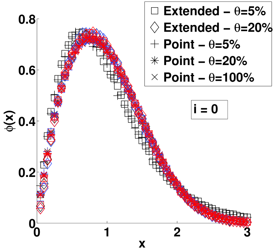
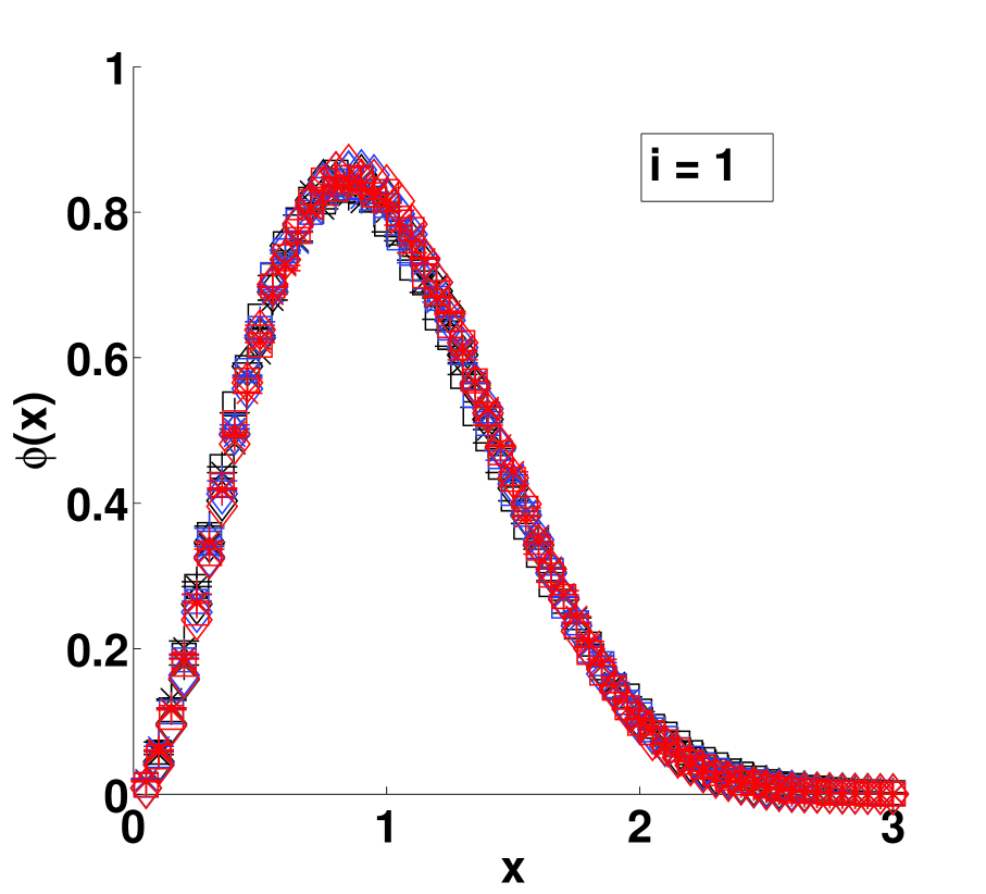
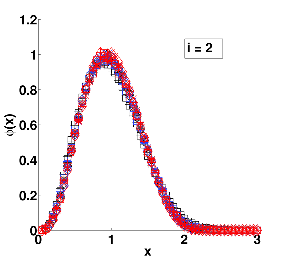
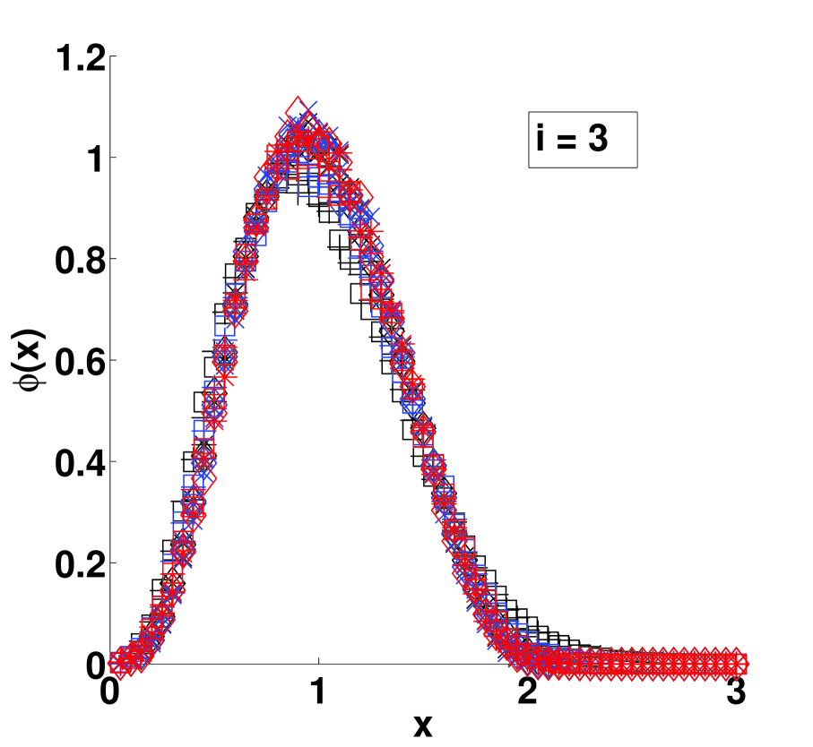
Figure 1: The scaled GSD $\phi$ for extended and point islands with $i=0$, $1$, $2$, $3$ and $\theta=5$%, $20$% and, in the point-island case only, $100$% obtained from MC simulations [$R=10^{7}$ (black), $R=10^{8}$ (blue) and $R=10^{9}$ (red)]. Note that the data for $R=10^{9}$ with $i=3$ and $\theta=100$% are not included.

    

    

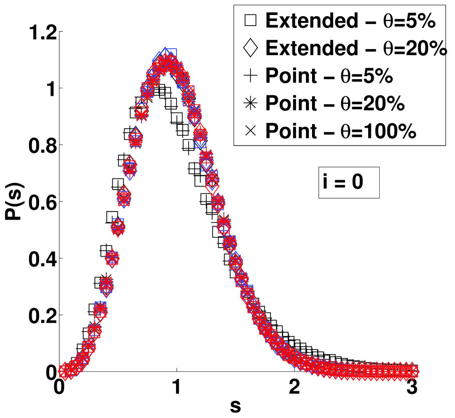
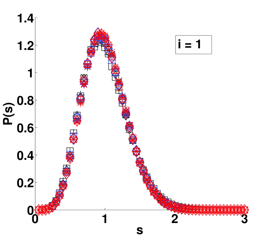
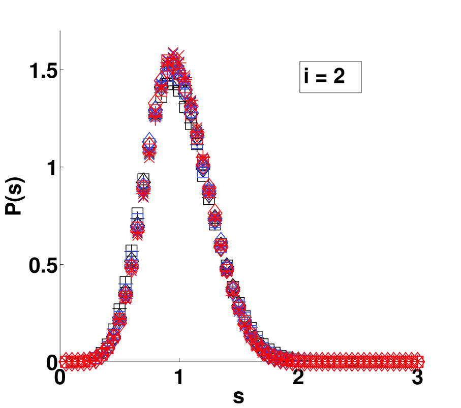
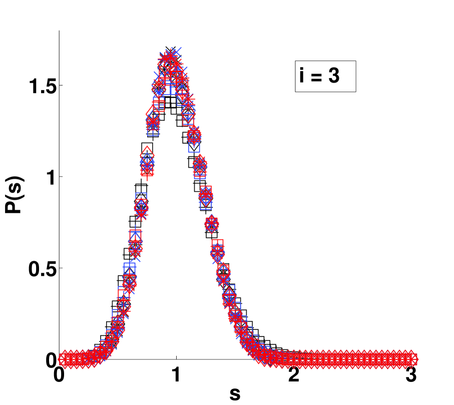
Figure 2: The scaled CZD $P$ for extended and point islands with $i=0$, $1$, $2$, $3$ and $\theta=5$%, $20$% and, in the point-island case only, $100$% obtained from MC simulations [$R=10^{7}$ (black), $R=10^{8}$ (blue) and $R=10^{9}$ (red)].

As is apparent from these results, we are a long way short of the limit where the 1-D substrate becomes saturated with islands. This limit is particularly problematic for point island models, since scaling breaks down as $\theta\rightarrow\infty$ and the CZD becomes singular Ratsch05 . Note that for point islands $\theta$ can be greater than $100$% whilst most of the substrate remains free of point islands, since they occupy a single site regardless of size. However we have been careful to ensure that we are far from this limit when we use simulation data to assess theoretical results below.

III THE MEAN-FIELD DFPE APPROACH FOR THE GAP SIZE DISTRIBUTION

Figure 3 shows some islands on the lattice, numbered according to their chronological age, along with their capture zones $C_{3}$, $C_{4}$ and $C_{5}$. Island $I_{3}$ has the capture zone of size $C_{3}=(g_{1}+g_{3})/2$, where $g_{1}$ and $g_{3}$ are the inter-island gaps to the left and right of $I_{3}$ respectively. $C_{3}$ represents the average growth rate of $I_{3}$, since any monomers deposited into $C_{3}$ are more likely to diffuse to $I_{3}$ than its neighbours $I_{1}$ and $I_{5}$.

Figure 3: The islands numbered $I_{1}-I_{5}$ on the one dimensional substrate. The gaps between the islands are labelled $g_{1}$, $g_{3}$, $g_{5}$ and $g_{4}$, and the capture zones of islands $I_{3}$, $I_{5}$, $I_{4}$ are labelled $C_{3}$, $C_{5}$ and $C_{4}$ respectively.

Referring to Figure 3, let us ask how the inter-island gap $g_{3}$ was created. It was formed by the nucleation of the youngest island in the picture, $I_{5}$, which occurred in the gap of size $(g_{3}+g_{5})$ between islands $I_{3}$ and $I_{4}$. Generalising, we will suppose that any randomly chosen gap with size $x$ (scaled to the average) in the system will have arisen by the fragmentation of a larger gap formed by combining the gap size of $x$ with a neighbouring gap of size $y$. In general we do not have the benefit of the chronological ages to guide us, so we make a mean field (MF) approximation for the size of the neighbouring gap, namely $y=1$. Denoting the probability of fragmenting a gap into proportions $a$ and $(1-a)$ by $f(a)$, we find the following distributional fixed point equation (DFPE) for the probability distribution function $\phi(x)$ of gaps $x\in[0,\infty)$:

$$x\stackrel{{\scriptstyle\triangle}}{{=}}a(1+x).$$ (3)

This convenient notation (exploited below) states that the distribution of the variates on the left is equal to that on the right Seba07 . Note that we have arrived at the same DFPE that Seba employed in his car-parking problem Seba07 , as discussed in Section I above. As in [PW, ], the DFPE leads to the Integral Equation (IE) for $\phi(x)$,

$$\phi(x)=\int_{0}^{\min(x,1)}\phi\left(\frac{x}{a}-1\right)\frac{f(a)}{a}da,$$ (4)

where the derivation of (4) can be found in Appendix A. Equation (3) states that the statistical distribution of gaps is unchanged by the fragmentation of all the gaps incremented in scaled size by one. Note that we neglect long-range chronological effects here, of the type apparent in Figure 3 for the creation of gap $g_{4}$ which arose from the nucleation of island $I_{4}$ and the fragmentation of gap $(g_{3}+g_{5}+g_{4})$. We will return to this point below.

In the aggregation regime, the probability $f(a)$ of fragmenting a gap into proportions $a$ and $(1-a)$ is found from the steady-state monomer density profile BM96 :

$$f(a)=\frac{a^{\alpha}(1-a)^{\alpha}}{B(\alpha+1,\alpha+1)}=\frac{(2\alpha+1)!}{(\alpha!)^{2}}a^{\alpha}(1-a)^{\alpha}.$$ (5)

Here $B(m,n)=\Gamma(m)\Gamma(n)/\Gamma(m+n)$ is the Beta function and $\alpha\in\mathbb{N}$ reflects the dominant nucleation mechanism. For nucleation triggered by deposition of monomers, $\alpha=i$ for $i=1,2,3\ldots$, whereas for nucleation resulting from the diffusion of mature monomers $\alpha=i+1$, $i=0,1,2,\ldots$ OGLM12 . At the asymptotic limit of large $R=D/F$ where $\theta=Ft$, the diffusion mechanism will dominate that of deposition. However, in practice, one cannot get to this limit in simulations or experiments (nor can we get to $t\rightarrow\infty$). Therefore, it is still valid to consider the behaviour whether one mechanism or the other dominates because this provides a good bracket to understand our MC data.

Figure 4: The evolution of gap size distribution under iteration of equation (4) with $i=1$. The solid lines are for $\alpha=i+1$ in equation (5), and the broken lines for $\alpha=i$, where the broken lines are shifted along the abscissa for clarity.

In Figure 4, by using an iteration scheme of the form

$$\phi_{n+1}(x)=F(\phi_{n}(x)),$$

where

$$F(\phi)=\int_{0}^{\min(x,1)}\phi\left(\frac{x}{a}-1\right)\frac{f(a)}{a}\ da,$$

we show the convergence of iterates of equation (4) starting from a rectangular distribution, with $f(a)$ given by equation (5). The limit satisfies the DFPE (3), and so is the form that we wish to compare to the scale-invariant GSD found in the MC simulations.

    

    

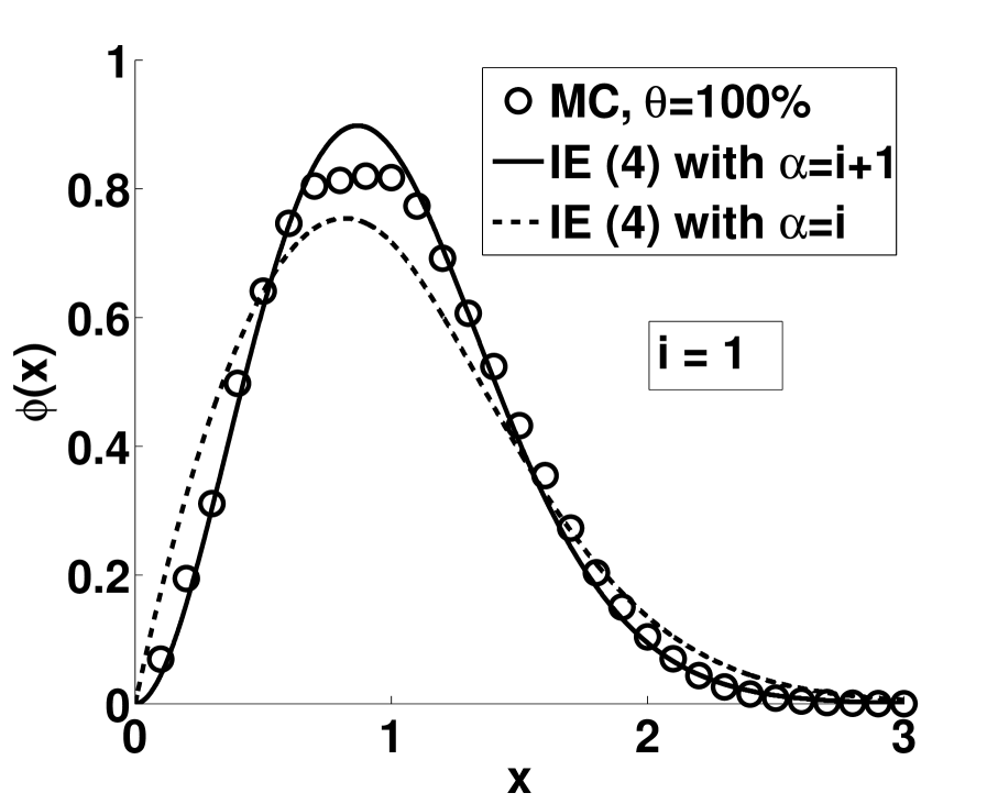
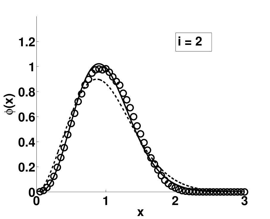
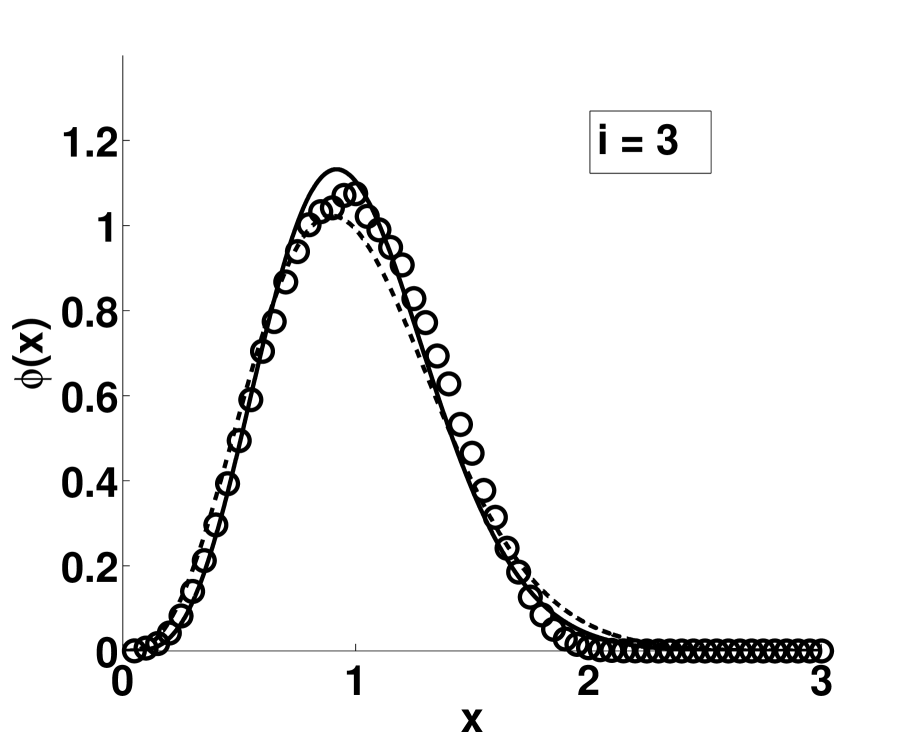
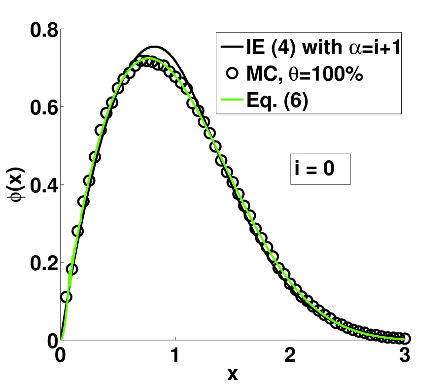
Figure 5: The GSDs compared to histograms of MC data OGLM12 , i.e. $R=8\times 10^{6}$, for various critical island size $i$, taken at nominal coverage $\theta=100$% . The solid curves are the converged solutions to equation (4) with $\alpha=i+1$ with $i=0,1,2,3$, and the broken lines are for $\alpha=i$ with $i=1,2,3$.

In Figure 5 we compare the numerically computed fixed points of equation (4), which we denote by $\phi_{\alpha}(x)$, with the GSDs of our MC simulations OGLM12 for various critical island size $i$. The comparison is rather good. For $i=1,2,3$, we see that the observed GSD lies between that of the $\alpha=i$ and $\alpha=i+1$ distributional fixed point solutions. This can be expected since we have found elsewhere that island nucleation is driven by both deposition events and purely diffusional fluctuations in monomer density OGLM12 . For spontaneous nucleation where $i=0$, only the $\alpha=i+1=1$ model is physically reasonable, since there is no possibility of a monomer depositing close to a pre-existing critical island of size $i$ in this case.

It is interesting to ask how the solutions to the DFPE equation (4) compare to those of the forward-propagated fragmentation theory equations, for which the asymptotic behaviours are known BM96 ; GLOM11 . Equation (4) can be rewritten as

$$\phi(x)=\int_{\max(0,x-1)}^{\infty}\phi(s)f\left(\frac{x}{s+1}\right)\frac{1}{s+1}\,ds,$$

from which it immediately follows using (5) that

$$\phi_{\alpha}(x)\sim kx^{\alpha}\mbox{ as }x\rightarrow 0,$$

for some constant $k$. This is the same small-size asymptotic behaviour found in the fragmentation theory approach GLOM11 ; OGLM12 . We could not obtain the large-size asymptotics for $\phi_{\alpha}(x)$ analytically. However, numerical analysis of the solutions in Figure 5 shows that they differ from those obtained by the fragmentation equation approach that we believe to be correct. The reason for this can be traced to the derivation of the DFPE (3), where not only do we adopt a MF approach for nearest neighbour gap sizes, but we also neglect longer-range correlations which are expected to be more prominent for larger gaps created early in the growth process. An example of this effect is, from Figure 3, is the creation of $g_{3}$ which arose from the nucleation $I_{3}$ and the fragmentation of gap of size ($g_{1}+g_{3}+g_{5}$). This particular type of nucleation event is not included in the DFPE (3), which assumes that gaps arise from the fragmentation of only two parents. Nevertheless, the results in Figure 5 show that this approach captures much of the essential physics for the GSDs.

For the $i=0$ case, it is possible to use the fragmentation approach combined with Treat’s results GLOM11 ; OGLM12 ; Treat to obtain the GSD function

$$\phi(x)=\frac{3x^{2}}{\Gamma(\frac{2}{3})\mu^{3}}\int_{(x/\mu)^{3}}^{\infty}u^{-4/3}e^{-u}\ du,$$ (6)

where

$$\mu=\frac{4}{3}\Gamma\left(\frac{2}{3}\right).$$

In Figure 5, we also plot Treat’s $\phi(z)$ from (6) to show how well our MF DFPE solutions work for $i=0$.

IV NON MEAN-FIELD DFPE APPROACHES FOR THE GAP SIZE DISTRIBUTION

IV.1 Unbiased DFPE

In deriving equations (3) and (4) in the previous section, we invoke a MF approximation for the size of the neighbouring gap, putting $y=1$. We could instead find the fixed point of the following DFPE that does not make a MF assumption:

$$x\stackrel{{\scriptstyle\triangle}}{{=}}a(x_{1}+x_{2}),$$ (7)

where the gaps $x_{1}$ and $x_{2}$ are, independently, drawn from the same distribution as $x$. As before $a$ is drawn from the probability distribution $f(a)$ of equation (5). Then instead of (4) we have the following IE for the GSD $\phi(x)$:

$$\phi(x)=\int_{0}^{1}\int_{0}^{x/a}\phi\left(\frac{x}{a}-x_{1}\right)\phi(x_{1})\frac{f(a)}{a}\ dx_{1}\ da,$$ (8)

The derivation is similar to that for the IE (4) shown in Appendix A. The convergence of iterates of (8) are shown in Figure 6.

    

    

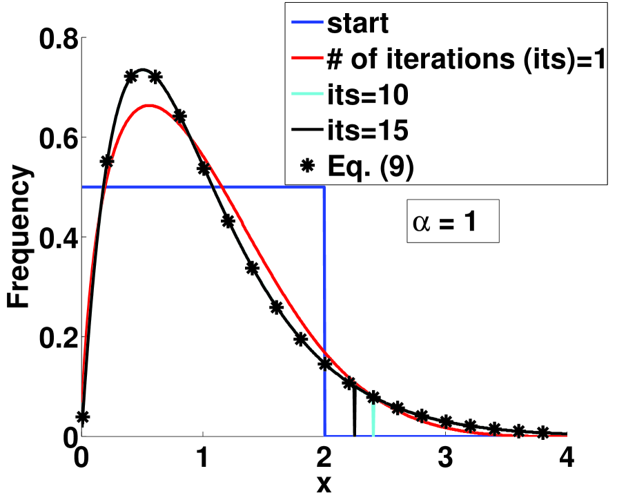
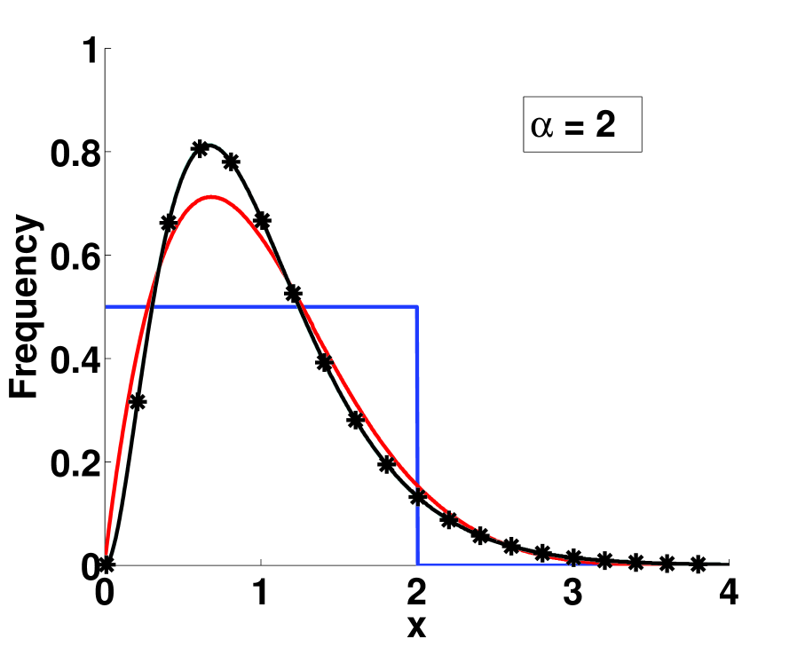
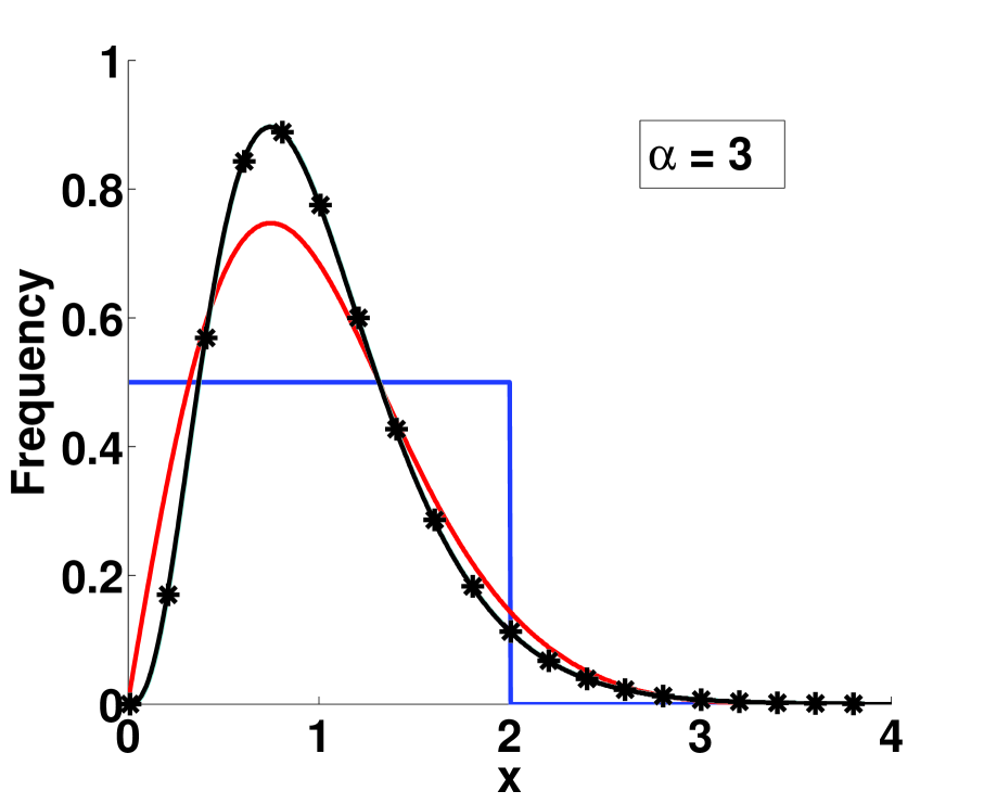
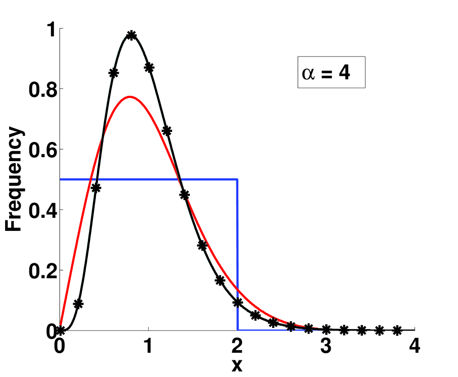
Figure 6: The evolution of gap size distribution under iteration of (8) with $\alpha=1$, $2$, $3$, $4$.

Equation (7) with $f(a)$ as in (5) is considered by Dufresne Duf96 , where it is shown that the fixed point is given by a gamma distribution. Explicitly the fixed point probability distribution is

$$\Gamma(\alpha+1,\nu,x)=\frac{x^{\alpha}\exp(-x/\nu)}{\Gamma(\alpha+1)\nu^{\alpha+1}}.$$

The mean of the above gamma distribution is $(\alpha+1)\nu$ and so, by setting $\nu=1/(\alpha+1)$, we rescale $x$ to unity to obtain

$$\phi_{\alpha}(x)=\frac{(\alpha+1)^{\alpha+1}}{\Gamma(\alpha+1)}x^{\alpha}e^{-(\alpha+1)x}.$$ (9)

Note that if we assume (9), then for small $x$ we obtain $\phi(x)\sim kx^{\alpha}$ for some constant $k$. In Figure 6, this gamma distribution is shown by the stars. It is apparent that the iterations converge to the form (9) and, as we see, it is not surprising to confirm the result obtained by Dufresne Duf96 .

IV.2 Fragmentation bias for the non-MF DFPE

The IE model presented in Eqn. (8) for the GSD is not appropriate for the island nucleation process, since we know from MC simulations OGLM12 that larger gaps are fragmented by nucleation events more often than smaller ones. We account for this effect in the following way. Referring to the non-MF DFPE Eqn. (7), we still wish to draw $x_{1}$ from $\phi(x_{1})$ in an unbiased way. However, $x_{2}$ is not unaffected by the value of $x_{1}$, and should not be drawn simply from $\phi(x_{2})$ as we did in Eqn. (8). Instead we draw it from a skewed distribution $(x_{1}+x_{2})^{2\alpha+1}.\phi(x_{2})$, reflecting the fact that a parent gap of size $x_{1}+x_{2}$ is fragmented with probability $(x_{1}+x_{2})^{2\alpha+1}$ from the integration of monomer density raised to the power $\alpha$ in the gap OGLM12 ; GLOM11 ; BM96 . With this, we derive the following, correctly biased non-MF IE:

$$\phi(x) =\int_{0}^{1}\int_{0}^{x/a}\phi\left(\frac{x}{a}-x_{1}\right)\phi(x_{1})f(a)$$

$$\times\frac{x^{2\alpha+1}}{a^{2\alpha+2}}\ da\ dx_{1}.$$ (10)

We now compare the fixed point probability distribution of equation (IV.2) with those from the MF approximation (4) and from (8) above; see Figure 7. Note that the effect of the bias is to skew the distribution away from that of equation (8), which over-represents small gaps, towards that of the MF approximation (see also Figure 5). The reason for this can be found in the biased form $(x_{1}+x_{2})^{2\alpha+1}.\phi(x_{2})$ which becomes more sharply peaked for larger $\alpha$, so its replacement by a single value in the MF equations is increasingly justified as $\alpha$ is increased. This behaviour is apparent in the results shown in Figure 7, and indeed even for $\alpha=1$ (corresponding to $i=0$) it is a very good approximation. Therefore this fragmentation bias vindicates the use of the MF approximation for the GSD, which allows us to proceed with some confidence to consider the CZD from the same MF perspective.

    

    

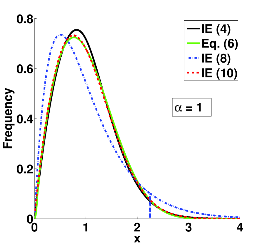
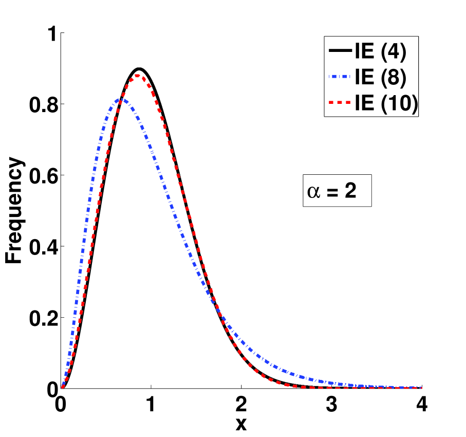
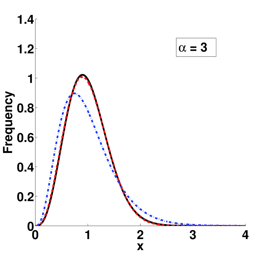
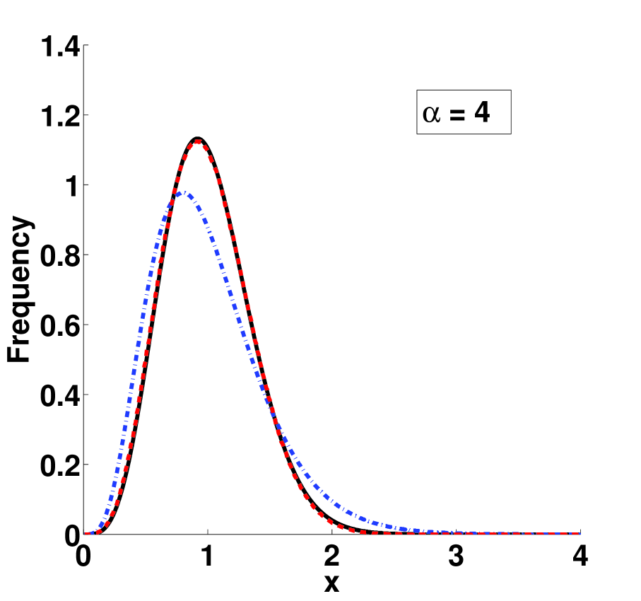
Figure 7: Comparison of the integral equations (4), (8) and (IV.2) and, for the $\alpha=1$ ($i=0$) case, Treat’s solution (6) for the various gap size models with $\alpha=1$, $2$, $3$, $4$.

V THE MEAN-FIELD DFPE FOR THE CAPTURE ZONE DISTRIBUTION

We turn now to consider the evolution of the capture zones in the system. One possible approach is to assume that neighbouring gaps are not correlated in size, so that the capture zone distributions (CZDs) can be calculated from convolutions of the related GSDs BM96 ; GLOM11 ; OGLM12 . However, here we prefer to progress in the same spirit as above, and use the MF approach to construct a DFPE for the capture zones, since this approach might be transferable to higher dimension substrates comment . Referring back to Figure 3, we see that the capture zone $C_{5}$ was created by the nucleation of island $I_{5}$. Prior to this, the zones $C_{3}$ and $C_{4}$ were larger, so that the creation of $C_{5}$ can be viewed as the fragmentation of part of $C_{3}$ (the part to the right of island $I_{3}$) and part of $C_{4}$ (to the left of $I_{4}$). In general we do not know how much of the neighbouring capture zones to take, nor indeed how large these zones are. However, we can again invoke a MF approximation for these nearest neighbour correlations to find the following DFPE for a general capture zone $c$:

$$c\stackrel{{\scriptstyle\triangle}}{{=}}\frac{1}{2}(a_{1}+a_{2})(1+c).$$ (11)

The proportions $a_{1}$ and $a_{2}$ are independently drawn from $f(a)$ of equation (5). An equivalent IE, like that of equation (4), can readily be identified for equation (11).

In Figure 8 we compare the CZDs obtained as fixed points of equation (11) with those from the MC simulations OGLM12 . Again we find excellent agreement, particularly for $i=0$ and $i=1$. We also plot the GWS (1) as a convenient analytical form. We see that the solution of equation (11) fits the data at least as well as, and in the case of $i=0$ much better than, the GWS. Whilst the validity of the GWS has been questioned as mentioned above in Section I, it is a useful benchmark for comparisons to MC data GPE11 ; OR11 .

    

    

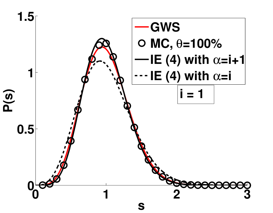
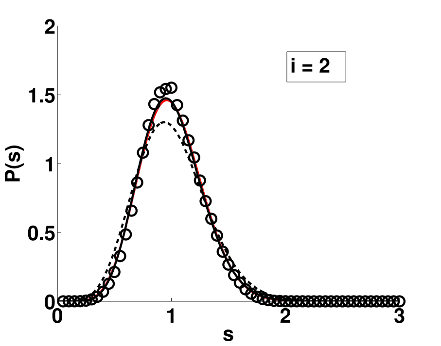
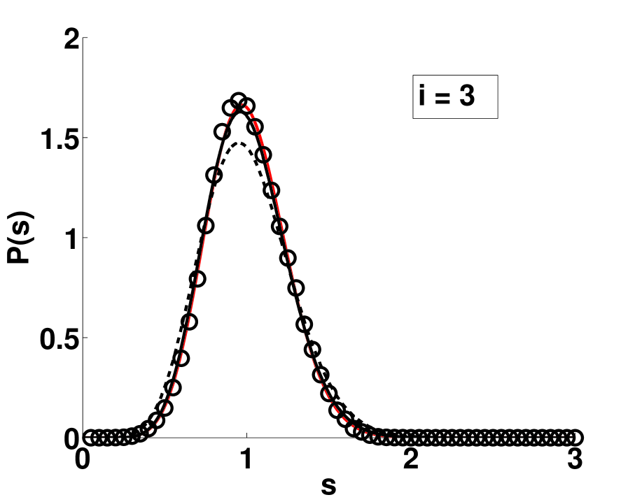
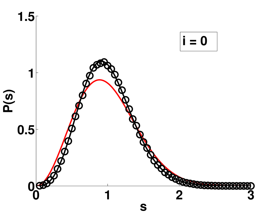
Figure 8: The CZDs compared to histograms of MC data OGLM12 for various critical island size $i$, taken at nominal coverage $\theta=100$%. The solid curves are the solutions to equation (11) for $\alpha=i+1$ with $i=0,1,2,3$, and the broken lines are for $\alpha=i$ with $i=1,2,3$.

We can easily quantify the performance of the solutions using the moments $S_{m}$ of the CZDs. Typically, when the GSDs, CZDs and/or ISDs are measured, the interest is the shape of the distribution and whether there is good data collapse to scaling forms which reveal nucleation and growth mechanisms. A distribution can be identified by a number of features such as the mean (first moment), the variance (second moment), the skewness (third moment) and the kurtosis (fourth moment) etc. In other words, the moments of a distribution can help to characterise its nature even if the full distribution is unknown, for example in a limited set of experimental data. Following [LJC10, ], from equation (11) we find the following recursive relationship:

$$S_{m}=\left(\frac{1}{2}\right)^{m}\sum_{k=0}^{m}\frac{m!}{k!(m-k)!}B_{m-k}B_{k}\sum_{p=0}^{m}\frac{m!}{p!(m-p)!}S_{p},$$ (12)

where

$$B_{m}=\frac{B(m+\alpha+1,\alpha+1)}{B(\alpha+1,\alpha+1)},$$

and $B(m,n)$ is the Beta function as in equation (5).

The moments of the GWS, Eqn. (1), are given by

$$G_{m}=\frac{\Gamma(i+3/2)^{m-1}\Gamma(i+(m+3)/2)}{(i+1)!^{m}}.$$ (13)

In Table 1 we compare the moments calculated from equations (12) and (13) alongside those taken from our MC simulations OGLM12 for $i=0,1,2,3$. These confirm the superiority of the DFPEs, notably for $\alpha=i+1$ implying a greater significance for nucleation driven by monomer diffusion.

$m$	$G_{m}$	$S_{m}$	$S_{m}$	MC
$i=0$
$2$	$1.178$	-	$1.138$	$1.134\pm 0.001$
$3$	$1.571$	-	$1.439$	$1.425\pm 0.001$
$4$	$2.313$	-	$1.989$	$1.949\pm 0.001$
$i=1$
$2$	$1.105$	$1.138$	$1.098$	$1.098\pm 0.001$
$3$	$1.325$	$1.439$	$1.305$	$1.307\pm 0.001$
$4$	$1.708$	$1.989$	$1.665$	$1.666\pm 0.001$
$i=2$
$2$	$1.074$	$1.098$	$1.076$	$1.066\pm 0.001$
$3$	$1.227$	$1.305$	$1.234$	$1.202\pm 0.001$
$4$	$1.483$	$1.665$	$1.500$	$1.425\pm 0.001$
$i=3$
$2$	$1.057$	$1.076$	$1.062$	$1.056\pm 0.001$
$3$	$1.175$	$1.234$	$1.190$	$1.169\pm 0.001$
$4$	$1.366$	$1.500$	$1.401$	$1.352\pm 0.001$

Table 1: Moments of the CZDs for $i=0$, $1$, $2$ and $3$ from the DFPE (12) with $\alpha_{n}=i+1$ or $\alpha_{n}=i$ (if appropriate), and from the MC simulations taken at $\theta=100$%.

VI SUMMARY AND CONCLUSIONS

In summary, we have presented distributional fixed point equations (DFPEs) and their equivalent, integral equations (IEs) for the nucleation of point islands in one dimension. The approach develops a new retrospective view of how the inter-island gaps and capture zones have developed from the fragmentation of larger entities.

To help validate our approach, we have carried out Monte Carlo (MC) simulations of the one-dimensional (1-D) point-island model for island nucleation and growth for $i=0,1,2,3$ and values of $R$ ranging from $10^{7}$ to $10^{9}$. We find that with higher values of $R$ there is good scale-invariance for the gap size distributions (GSDs) and capture zone distributions (CZDs) at coverages ($\theta\leq 20$%), where the scaling form depends on critical island size $i$. Significantly, we also find little to distinguish these distributions from those of simulations with more realistic extended islands, so that whilst our subsequent DFPE development is focused on point islands, it can equally apply to the extended island case, at least for low substrate coverage.

We first developed a mean field (MF) approach to the nucleation of gaps between islands on the substrate, arguing for the simple DFPE of Eqn. (3) and its associate IE of Eqn. (4). We found good comparisons between the converged solutions and the MC data, suggesting that the model has a reasonable physical basis. Exploring the idea further, we next considered the non-MF DFPE of Eqn. (7). Without using any selection bias for the parents we showed that solutions to the associated IE Eqn. (8) are gamma distributions Duf96 . However, including the bias towards fragmenting large parents arising from the fragmentation probability $f(a)$ in Eqn. (5), we found that the solutions are drawn back to those of the initial MF version, justifying this approximation. Interestingly, even for $i=0$ we found that the MF solution works well and is reasonably close to the exact fragmentation theory solution for this case Treat .

We also considered the DFPE (11) and IE in the form of (4) for the CZD, following in the same MF spirit. This allowed a closed form for the CZD to be developed, unlike previous approaches BM96 ; GLOM11 ; OGLM12 ; GPE11 where the CZD is explicitly derived from convolution of the GSD. The solutions to our equations compare well to MC simulation data, performing at least as well as the Generalised Wigner Surmise (GWS) PE07 , and notably better for the case of $i=0$. The recursive form of DFPE also allowed calculation of moments of the distributions, values which might be useful in the future for assessing limited experimental data.

Our presentation of DFPEs and associated IEs for island nucleation in 1-D provides a fresh perspective on why scaling emerges in this non-equilibrium growth system. Furthermore, we hope that a similar approach might be possible in higher dimensions too. Whilst the utility of inter-island gaps is perhaps limited to the 1-D case, capture zones still underpin island growth rates in higher dimensions BM96 ; MR00 ; EB02 ; Li10 , so that it might be possible in future work to find an equivalent closed-form DFPE for the CZD on higher dimensional substrates.

Appendix A Derivation of the integral equation (4)

Following the analysis PW ; Seba07 , we obtain an IE which is equivalent to the DFPE (3)

Proposition A.1

For the gap size distribution, $\phi(x)$, the following integral equation

$$\phi(x)=\int_{0}^{\min(x,1)}\phi\left(\frac{x}{a}-1\right)\frac{f(a)}{a}da,$$

is derived from the distributional fixed point equation (3).

We give a proof of this proposition. Let $\Phi$ be the cumulative distribution function (CDF) that corresponds to the density function $\phi$. Then $\Phi(x)=0$ for all $x\leq 0$ and we have

$$\Phi(x) =Prob[x_{1}\leq x]$$

$$=Prob[a(1+x_{1})\leq x]$$

$$=E[\ Prob[a(1+x_{1})\leq x\ |\ a]\ ]$$

$$=\int_{0}^{1}Prob[a(1+x_{1})\leq x]f(a)da$$

$$=\int_{0}^{1}Prob[x_{1}\leq x/a-1]f(a)da$$

$$=\int_{0}^{1}\Phi(x/a-1)H(x/a-1)f(a)da,$$

where $H(\cdot)$ is the Heaviside function since $\Phi(x_{1})=Prob[x_{1}\leq a]$ and since $\Phi(x)=0$ if $x\leq 0$. Hence the CDF satisfies

$$\Phi(x)=\int_{0}^{\min(x,1)}\Phi\left(\frac{x}{a}-1\right)f(a)da.$$ (14)

The change variables to $w=x/a-1$ yields

$$\Phi(x)=x\int_{\max(0,x-1)}^{\infty}\Phi(w)f\left(\frac{x}{w+1}\right)\frac{1}{(w+1)^{2}}\ dw.$$

Given the form (5), the differentiability of $f$ means that we can use the Leibniz rule to establish that $\Phi^{\prime}(x)=\phi(x)$ exists for each of the cases $x>1$ and $x<1$. Returning to equation (14), we obtain, for $x<1$,

$$\phi(x)=\Phi^{\prime}(x) =\Phi(0)f(x)+\int_{0}^{x}\Phi^{\prime}\left(\frac{x}{a}-1\right)\frac{f(a)}{a}\ da$$

$$=\int_{0}^{x}\phi\left(\frac{x}{a}-1\right)\frac{f(a)}{a}\ da,$$

and, for $x>1$,

$$\phi(x)=\Phi^{\prime}(x)=\int_{0}^{1}\phi\left(\frac{x}{a}-1\right)\frac{f(a)}{a}\ da.$$

Taking left-sided and right-sided limits, we deduce that

$$\phi(1)=\lim_{x\rightarrow 1}\phi(x)=\int_{0}^{1}\phi\left(\frac{1}{a}-1\right)\frac{f(a)}{a}\ da,$$

and the stated result follows.

- (1) J. G. Amar and F. Family F, Phys. Rev. Lett. 74, 2066 (1995).
- (2) P. A. Mulheran, Europhys. Lett. 65, 379 (2004).
- (3) J. A. Venables, Philos. Mag. 27, 693 (1973).
- (4) M. C. Bartelt and J. W. Evans, Phys. Rev. B 46, 12675 (1992).
- (5) J. G. Amar, F. Family F and P. -M. Lam, Phys. Rev. B 50, 8781 (1994).
- (6) G. S. Bales and D. C. Chrzan, Phys. Rev. B 50, 6057 (1994).
- (7) J. A. Blackman and A. Wilding, Europhys. Lett. 16, 115 (1991).
- (8) C. Ratsch, A. Zangwill, P. Smilauer, and D.D. Vvedensky, Phys. Rev. Lett. 72, 3194 (1994).
- (9) P. A. Mulheran and J. A. Blackman Philo. Mag. Lett. (1995); P.A. Mulheran and J.A. Blackman, Phys. Rev. B 53, 10261 (1996).
- (10) M. C. Bartelt and J. W. Evans, Phys. Rev. B 54, R17359 (1996).
- (11) P. A. Mulheran and D. A. Robbie, Europhys. Lett. 49, 617 (2000).
- (12) J. G. Amar, M. N. Popescu and F. Family, Phys. Rev. Lett. 86, 3092 (2001).
- (13) J. W. Evans and M. C. Bartelt, Phys. Rev. B 66, 235410 (2002).
- (14) A. Pimpinelli and T. L. Einstein, Phys. Rev. Lett. 99, 226102 (2007).
- (15) T. J. Oliveira and F. D. A. Aarao Reis, Phys. Rev. B 83, 201405 (2011).
- (16) M. Li, Y. Han and J. W. Evans, Phys. Rev. Lett. 104, 149601 (2010).
- (17) F. Shi, Y. Shim and J.G. Amar, Phys. Rev. E 79, 011602 (2009).
- (18) J. A. Blackman and P. A. Mulheran, Phys. Rev. B 54, 11681 (1996).
- (19) M. Grinfeld, W. Lamb, P. A. Mulheran and K. P. O’Neill, J. Phys. A 45, 015002 (2012).
- (20) D. L. Gonzalez, A. Pimpinelli and T. L. Einstein, Phys. Rev. E 84, 011601 (2011).
- (21) K. P. O’Neill, M. Grinfeld, W. Lamb and P. A. Mulheran, Phys. Rev. E 85, 021601 (2012).
- (22) A. Pimpinelli and T. L. Einstein, Response to comment on “Capture-zone scaling in island nucleation: universal fluctuation behaviour”, Phys. Rev. Lett 104 (2010), 149602-1.
- (23) P. Seba, Acta Physica Polonica A 112, 681 (2007).
- (24) C. Ratsch, Y. Landa and R. Vardavas, The asymptotic scaling limit of point island models for epitaxial growth, Surf. Sci. 578 (2005), 196–202.
- (25) M. D. Penrose and A. R. Wade, Adv. Appl Prob. 6, 691 (2004).
- (26) R. P. Treat, On the similarity solution of the fragmentation equation, J. Phys. A 30 (1997), 2519–2543.
- (27) D. Dufresne, On the stochastic equation and a property of gamma distributions, Bernoulli 2 (1996), 287-291.
- (28) The advantage of the MF approach we adopt here is that it leads to a closed form for the capture zones in Equation (11), whereas the convolution of the GSD does not.
- (29) M. Lallouache, A. Jedidi and A. Chakraborti, arXiv:1004.5109.