Stabilization of an arbitrary profile
for an ensemble of half-spin systems

Abstract

We consider the feedback stabilization of a variable profile for an ensemble of non interacting half spins described by the Bloch equations. We propose an explicit feedback law that stabilizes asymptotically the system around a given arbitrary target profile. The convergence proof is done when the target profile is entirely in the south hemisphere or in the north hemisphere of the Bloch sphere. The convergence holds for initial conditions in a $H^{1}$ neighborhood of this target profile. This convergence is shown for the weak $H^{1}$ topology. The proof relies on an adaptation of the LaSalle invariance principle to infinite dimensional systems. Numerical simulations illustrate the efficiency of these feedback laws, even for initial conditions far from the target profile.

, ,

1 Introduction

Ensemble controllability as introduced in Li and Khaneja (2009) is an interesting control theoretic notion well adapted to nuclear magnetic resonance (NMR) systems (see, e.g., Li and Khaneja (2006) and the reference herein). In Beauchard et al. (2010) some controllability issues of such NMR systems are investigated using open-loop controls involving Dirac-combs. In Beauchard et al. (2011) such open-loop Dirac-combs are combined with Lyapunov stabilizing feedback to ensure closed-loop convergence towards a target profile that is one of the two steady-states, the south and north poles of the Bloch sphere. In this note, we extend this Lyapunov design to arbitrary target profiles and prove its local convergence for weak $H^{1}$ topology when the target profile lies entirely in the south hemisphere or in the north hemisphere.

We consider an ensemble of non interacting half-spins in a static field $(0,0,B_{0})^{t}$ in $\mathbb{R}^{3}$, subject to a transverse radio frequency field $(\tilde{u}_{1}(t),\tilde{u}_{2}(t),0)^{t}$ in $\mathbb{R}^{3}$ (the control input). The ensemble of half-spins is described by the magnetization vector $M\in\mathbb{R}^{3}$ depending on time $t$ but also on the Larmor frequency $\omega=-\gamma B_{0}$ ($\gamma$ is the gyromagnetic ratio). It obeys to the Bloch equation:

$$\frac{\partial M}{\partial t}(t,\omega)=(\tilde{u}_{1}(t)e_{1}+\tilde{u}_{2}(t)e_{2}+\omega e_{3})\wedge M(t,\omega),$$ (1)

where $-\infty<\omega_{*}<\omega^{*}<+\infty$, $\omega\in(\omega_{*},\omega^{*})$, $(e_{1},e_{2},e_{3})$ is the canonical basis of $\mathbb{R}^{3}$, $\wedge$ denotes the wedge product on $\mathbb{R}^{3}$. The equation (1) is an infinite dimensional bilinear control system. The state is the $\omega$-profile $M$, where, for every $\omega\in(\omega_{*},\omega^{*})$, $M(t,\omega)\in\mathbb{S}^{2}$ (the unit sphere of $\mathbb{R}^{3}$). The two control inputs $\tilde{u}_{1}$ and $\tilde{u}_{2}$ are real valued.

We propose here a first answer to the local stabilization of an arbitrary profile: given an arbitrary target profile $M_{f}:(\omega_{*},\omega^{*})\rightarrow{\mathbb{S}}^{2}$, define an explicit control law $(\tilde{u}_{1}(t,M),\tilde{u}_{2}(t,M))$, a neighborhood $U$ of $M_{f}$ (in some space of functions to be determined), a diverging sequence of times $(t_{n})_{n\in\mathbb{N}}$, such that, for every initial condition $M^{0}\in U$, the solution of the closed loop system is uniquely defined and satisfies

$$\lim\limits_{n\rightarrow+\infty}\|M(t_{n},.)-M_{f}(.)\|_{L^{\infty}(\omega_{*},\omega^{*})}=0.$$

In this note, the Lyapunov feedback proposed in Beauchard et al. (2011) is adapted to provide a constructive answer to this question. Section 2 is devoted to control design and closed-loop simulations. In section 3 we state and prove the main convergence result, theorem 1.

2 Lyapunov $H^{1}$ approach

2.1 Some preliminaries

Let us recall the concept of a solution for (1) when the control input $u$ contains Dirac distributions. When $\tilde{u}_{1},\tilde{u}_{2}\in L^{1}_{loc}(\mathbb{R})$, then, for every initial condition $M_{0}\in L^{2}((\omega_{*},\omega^{*}),\mathbb{R}^{3})$, the equation (1) has a unique weak solution $M\in C^{0}([0,+\infty),L^{2}((\omega_{*},\omega^{*}),\mathbb{R}^{3}))$. Denote by $\delta(t-a)$ the Dirac distribution located at $t=a$. When $\tilde{u}_{1}=\alpha\delta(t-a)+u_{1}^{\sharp}$ and $\tilde{u}_{2}=u_{2}^{\sharp}$ where $u_{j}^{\sharp}\in L^{1}_{loc}(\mathbb{R})$, $\alpha>0$ and $a\in(0,+\infty)$, then the solution is the classical solution on $[0,a)$ and $(a,+\infty)$, it is discontinuous at the time $t=a$, with an explicit discontinuity given by an instantaneous rotation of angle $\alpha$ around the axis $\mathbb{R}e_{1}$

$$M(a^{+},\omega)=\left(\begin{array}[]{ccc}1&0&0\\ 0&\cos(\alpha)&-\sin(\alpha)\\ 0&\sin(\alpha)&\cos(\alpha)\end{array}\right)M(a^{-},\omega).$$

The symbol $\|.\|$ (resp. $\langle.,.\rangle$) denotes the Euclidian norm (resp. scalar product) on $\mathbb{R}^{3}$ and the associated operator norm on $\mathcal{M}_{3}(\mathbb{R})$.

2.2 Transformation into a driftless system

As in Beauchard et al. (2011) we consider a control with an “impulse-train” structure

$$\tilde{u}_{1}=u_{1}+\sum_{k=1}^{+\infty}\pi~{}\delta(t-kT),\quad\tilde{u}_{2}=(-1)^{\epsilon(t)}u_{2}$$ (2)

where $\epsilon(t):=E(t/T)$, for some period $T>0$ and $E(\gamma)$ denotes the integer part of the real number $\gamma$. The new controls $u_{1},u_{2}$ belong to $L^{1}_{loc}(\mathbb{R})$. Considering the change of variable

$$M_{1}(t,\omega):=P(t)M(t,\omega)\text{ where }P(t):=\left(\begin{array}[]{ccc}1&0&0\\ 0&\epsilon(t)&0\\ 0&0&\epsilon(t)\end{array}\right)$$ (3)

one gets the following dynamics

$$\frac{\partial M_{1}}{\partial t}(t,\omega)=[u_{1}(t)e_{1}+u_{2}(t)e_{2}+\epsilon(t)\omega]\wedge M_{1}(t,\omega).$$ (4)

The application of impulses at $t=kT$, by changing the sense of rotation of the null input solution, is expected to reduce the dispersion in the closed loop system. Since $M(t,\omega)=M_{1}(t,\omega)$ for every $t\in[2kT,(2k+1)T]$, any convergence result on $M_{1}(t)$ when $t\rightarrow+\infty$ provides a convergence result on $M$.

The first step of the control design consists in putting the system (4) in driftless form. The new function

$$M_{2}(t,\omega):=\exp[\sigma(t)\omega S]M_{1}(t,\omega)$$

where

$$\sigma(t):=\int_{0}^{t}\epsilon(s)ds,\quad S:=\left(\begin{array}[]{ccc}0&1&0\\ -1&0&0\\ 0&0&0\end{array}\right),$$ (5)

solves

$$\frac{\partial M_{2}}{\partial t}(t,\omega)=\sum_{i=1}^{2}u_{i}(t)\Big{[}\exp(\sigma(t)\omega S)e_{i}\Big{]}\wedge M_{2}(t,\omega).$$ (6)

Since $\sigma(2kT)=0,\forall k\in\mathbb{N}$, any convergence on $M_{2}(t)$ when $t\rightarrow+\infty$ provides a convergence on $M_{1}(2kT)$ when $k\rightarrow+\infty$.

2.3 Transformation of the target profile

The second step of the control design consists in transforming a convergence to a variable profile $M_{f}$ into a convergence to the constant profile $-e_{3}$, for which we developed tools in the previous work Beauchard et al. (2011). It relies on the following proposition.

Proposition 1.

There exists $C>0$ such that, for all $M_{f}\in H^{1}((\omega_{*},\omega^{*}),{\mathbb{S}}^{2})$, there exists $R\in H^{1}((\omega_{*},\omega^{*}),SO_{3}(\mathbb{R}))$ satisfying

$$R(\omega)M_{f}(\omega)=-e_{3},\quad\forall\omega\in[\omega_{*},\omega^{*}],$$ (7)

$$\|R\|_{H^{1}}\leqslant C\|M_{f}\|_{H^{1}}.$$ (8)

Proof: Let $M_{f}\in H^{1}((\omega_{*},\omega^{*}),{\mathbb{S}}^{2})$ and set $f(\omega):=M_{f}^{\prime}(\omega)\wedge M_{f}(\omega)$. Denote by $A(\omega)$ the skew-symmetric operator defined by $\mathbb{R}^{3}\ni M\mapsto f(\omega)\wedge M\in\mathbb{R}^{3}$. Consider the Cauchy problem

$$\frac{d}{d\omega}R=RA(\omega)\text{ on }[\omega_{*},\omega^{*}]\text{ with }R(\omega_{*})=R_{*}$$

where $R_{*}$ is any rotation sending $M_{f}(\omega_{*})$ to $-e_{3}$: $R_{*}M_{f}(\omega_{*})=-e_{3}$. Since $\omega\mapsto A(\omega)$ is $L^{2}$ the solution $R$ is well defined, unique and belongs to $H^{1}((\omega_{*},\omega^{*}),{\mathbb{S}}^{2})$. Direct computations show that $\frac{d}{d\omega}(RM_{f})=0$. Thus $R(\omega)M_{f}(\omega)\equiv-e_{3}$. Moreover, $\|R(\omega)\|=1$ and $\|R^{\prime}(\omega)\|=\|A(\omega)\|=\|M_{f}^{\prime}(\omega)\|$ for all $\omega\in[\omega_{*},\omega^{*}]$, which proves (8). $\Box$.

Let us consider a target profile $M_{f}\in H^{1}((\omega_{*},\omega^{*}),{\mathbb{S}}^{2})$. Take $R\in H^{1}((\omega_{*},\omega^{*}),SO_{3}(\mathbb{R}))$ given by the above proposition. To any solution $M_{2}$ of (6), we associate the function

$$N(t,\omega):=R(\omega)M_{2}(t,\omega),\forall\omega\in[-\omega_{*},\omega^{*}].$$ (9)

This function solves the equation

$$\frac{\partial N}{\partial t}(t,\omega)=\sum_{i=1}^{2}u_{i}(t)\Big{[}F(t,\omega)e_{i}\Big{]}\wedge N(t,\omega)$$ (10)

where

$$F(t,\omega):=R(\omega)\exp(\sigma(t)\omega S).$$ (11)

The convergence of $N(t,\omega)$ to $-e_{3}$ as $t\rightarrow+\infty$ is equivalent to the convergence of $M_{2}(t,\omega)$ to $M_{f}(\omega)$ as $t\rightarrow+\infty$.

2.4 Lyapunov feedback

Let us consider the following Lyapunov-like functional

$$~{}\mathcal{L}(N):=\frac{\|N+e_{3}\|_{H^{1}}^{2}}{2}\\ =\int\limits_{\omega_{*}}^{\omega^{*}}\Big{(}\frac{1}{2}\Big{\|}\frac{\partial N}{\partial\omega}\Big{\|}^{2}+1+\langle N,e_{3}\rangle\Big{)}d\omega.$$ (12)

The function $\mathcal{L}$ is defined for any $N\in H^{1}((\omega_{*},\omega^{*}),{\mathbb{S}}^{2})$ and takes its minimal value on this space at the point $N=-e_{3}$ with $\mathcal{L}(-e_{3})=0$. For any solution of (10), some computations show that

$$\frac{d\mathcal{L}}{dt}[N(t)]=\sum_{i=1}^{2}u_{i}(t)H_{i}[t,N(t)]$$

where, for $i=1,2$ one has

$$H_{i}[t,N]:=\int_{\omega_{*}}^{\omega^{*}}\bigg{[}\left\langle\frac{dN}{d\omega}(\omega),\Big{(}\frac{\partial F}{\partial\omega}(t,\omega)e_{i}\Big{)}\wedge N(\omega)\right\rangle\\ +\left\langle e_{3},\Big{(}F(t,\omega)e_{1}\Big{)}\wedge N(\omega)\right\rangle\bigg{]}d\omega.$$

Hence, with the feedback laws

$$u_{i}(t,N):=-H_{i}[t,N],\forall i\in\{1,2\},$$ (13)

it follows that

$$\frac{d\mathcal{L}}{dt}[N(t)]=-u_{1}(t,N)^{2}-u_{2}(t,N)^{2}\leqslant 0.$$ (14)

As in Beauchard et al. (2011), we have the following result.

Proposition 2.

For every initial condition $N_{0}\in H^{1}((\omega_{*},\omega^{*}),{\mathbb{S}}^{2})$, the closed loop system (10), (13) has a unique solution $N\in C^{1}\left([0,\infty),H^{1}\left((\omega_{*},\omega^{*}),\mathbb{R}^{3}\right)\right)$ such that $N(0)=N_{0}$.

2.5 Closed-loop simulations

We assume here $\omega_{*}=0$, $\omega^{*}=1$ and we solve numerically the $T$-periodic system (1) with the feedback law $(\tilde{u}_{1},\tilde{u}_{2})$ given by (2), (13). The closed-loop simulation is performed for $t\in[0,T_{f}]$, $T_{f}=20T$ and $T=2\pi/(\omega^{*}-\omega_{*})$. The $\omega$-profile $[\omega_{*},\omega^{*}]\ni\omega\mapsto(x(t,\omega),y(t,\omega),z(t,\omega))$ is discretized $\{1,\ldots,N+1\}\ni k\mapsto(x_{k}(t),y_{k}(t),z_{k}(t))$ with a regular mesh of step $\epsilon_{N}=\frac{\omega^{*}-\omega_{*}}{N}$ with $N=100$. In other words, one has a set of discrete values $\{\omega_{i},i=1,\ldots,N+1\}$, where $\omega_{i}=\omega_{*}+(i-1)\epsilon_{N}$.

We have checked that the closed-loop simulations are almost identical for $N=100$ and $N=200$. In the feedback law (16), the integral versus $\omega$ is computed assuming that $(x,y,z)$ and $(x^{\prime},y^{\prime},z^{\prime})$ are constant over $](k-\tfrac{1}{2})\epsilon_{N},(k+\tfrac{1}{2})\epsilon_{N}[$, their values being $(x_{k},y_{k},z_{k})$ and $\left(\tfrac{x_{k+1}-x_{k-1}}{2\epsilon_{N}},\tfrac{y_{k+1}-y_{k-1}}{2\epsilon_{N}},\frac{z_{k+1}-z_{k-1}}{2\epsilon_{N}}\right)$. The obtained differential system is of dimension $3(N+1)$. It is integrated via an explicit Euler scheme with a step size $h=T/1000$. We have tested that $h=T/2000$ yields almost the same numerical solution at $t=T_{f}=20T$. After each time-step the new values of $(x_{k},y_{k},z_{k})$ are normalized to remain in ${\mathbb{S}}^{2}$. The initial $\omega$-profile $M_{0}(\omega)$ of $(x,y,z)\in{\mathbb{S}}^{2}$ is given by $x_{0}=0,y_{0}=-\sqrt{1-z_{0}^{2}}$, where $z_{0}=-\cos(\frac{\pi}{8})+0.05\left(1-\cos(\frac{\pi}{8})\cos(\omega\frac{\pi}{2})\right)$. The desired final profile $M_{f}(\omega)$ is given by $x_{f}=-\sqrt{1-z_{f}^{2}},y_{f}=0$, where $z_{f}=-\cos(\frac{\pi}{16})+0.1\left(1-\cos(\frac{\pi}{16})\sin(\omega\frac{\pi}{4})\right)$.

The map $R(\omega)$ is constructed for the discrete set $\{\omega_{i},i=1,\ldots,N+1\}$, in the following way. For $i=1$, one takes $r_{3}(\omega_{1})=M_{0}(\omega_{1})$. Now choose a vector $\theta$ among the vectors of the canonical basis in a way that $\langle\theta,M_{f}(\omega_{1})\rangle$ is the minimum value. Construct $r_{2}(\omega_{1})=\frac{1}{\|\theta\wedge r_{3}(\omega_{1})\|}\left(\theta\wedge r_{3}(\omega_{1})\right)$. Then one may take $r_{1}(\omega_{2})=r_{2}(\omega_{2})\wedge r_{3}(\omega_{2})$. Now, for $i=2,3,\ldots,N+1$ one chooses $r_{3}(\omega_{i})=M_{0}(\omega_{i})$, $\theta=-r_{1}(\omega_{i-1})$, $r_{2}(\omega_{i})=\frac{1}{\|\theta\wedge r_{3}(\omega_{i})\|}\left(\theta\wedge r_{3}(\omega_{i})\right)$ and $r_{1}(\omega_{i})=r_{2}(\omega_{i})\wedge r_{3}(\omega_{i})$, and so on. The orthogonal matrix $\bar{R}(\omega)$ formed by the column vectors $r_{1}$, $r_{2}$, $r_{3}$ is then transposed to obtain $R(\omega)$.

Figures 1 and 2 summarize the main convergence issues for these choices of initial profile $M_{0}$ and of the desired final profile $M_{f}$. The convergence speed is rapid at the beginning and tends to decrease at the end. We start with ${\mathcal{L}}(0)\approx 0.1929$. We get ${\mathcal{L}}(20T)\approx 0.0032$. This numerically observed convergence is confirmed by Theorem 1 here below.

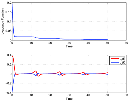
Figure 1: Lyapunov function $\mathcal{L}(t)$ defined by (12) and the closed-loop control $({u}_{1},{u}_{2})$ defined by (13)

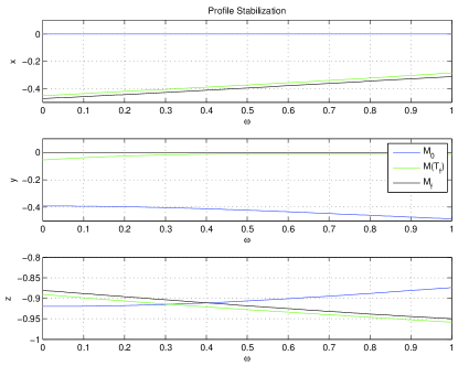
Figure 2: Initial ($t=0$) and final ($t=T_{f}$) $\omega$-profiles for $x$, $y$ and $z$ solutions of the closed-loop system 1 with the feedback (2), (13).

3 Main Result

3.1 Local stabilization

Theorem 1.

For every $M_{f}\in H^{1}((\omega_{*},\omega^{*}),{\mathbb{S}}^{2})$ with

$$\langle M_{f}(\omega),e_{3}\rangle\neq 0,\forall\omega\in[\omega_{*},\omega^{*}],$$ (15)

there exists $\delta_{1}>0$ such that, for every $N_{0}\in H^{1}((\omega_{*},\omega^{*}),{\mathbb{S}}^{2})$ with $\|N_{0}+e_{3}\|_{H^{1}}\leq\delta_{1}$, the solution of the closed loop system (10), (13) with initial condition $N(0,\omega)=N_{0}(\omega)$ satisfies $N(t)\rightharpoonup-e_{3}$ weakly in $H^{1}(\omega_{*},\omega^{*})$ when $t\rightarrow+\infty$.

The above theorem has the following corollary.

Corollary 1.

For every $M_{f}\in H^{1}((\omega_{*},\omega^{*}),{\mathbb{S}}^{2})$ with (15), there exists $\delta_{2}>0$ such that, for every $M_{0}\in H^{1}((\omega_{*},\omega^{*}),{\mathbb{S}}^{2})$ with $\|M_{0}-M_{f}\|_{H^{1}}<\delta_{2}$, the solution of the system (1) with the initial condition $M(0,\omega)=M_{0}(\omega)$ and the feedback law given by (2), (13) satisfies $M((2kT)^{+})\rightharpoonup M_{f}$ weakly in $H^{1}$ when $k\rightarrow+\infty$. In particular,

$$\lim\limits_{k\rightarrow+\infty}\|M((2kT)^{+},.)-M_{f}\|_{L^{\infty}(\omega_{*},\omega^{*})}=0.$$

The remaining part of this section is devoted to the proof of Theorem 1

3.2 LaSalle invariant set

The first step of our proof consists in checking that, locally, the invariant set is reduced to $\{-e_{3}\}$.

Proposition 3.

For every $M_{f}\in H^{1}((\omega_{*},\omega^{*}),{\mathbb{S}}^{2})$ with (15), there exists $\delta>0$ such that, for every $N_{0}\in H^{1}((\omega_{*},\omega^{*}),{\mathbb{S}}^{2})$ with $\|N_{0}+e_{3}\|<\delta$, the map $t\mapsto\mathcal{L}[N(t)]$ is constant on $[0,+\infty)$ if and only if $N_{0}=-e_{3}$.

Proof: Let us assume that $t\mapsto\mathcal{L}[N(t)]$ is constant. Then $u_{1}=u_{2}=0$ and $N(t,\omega)\equiv N_{0}(\omega)$ (see (14) and (10)). Thus, for every $j\in\{1,2\}$ and $t\in[0,+\infty)$

$$\begin{array}[]{rl}0=&\int_{\omega_{*}}^{\omega^{*}}\left[\left\langle N_{0}^{\prime}(\omega),\Big{(}\frac{\partial F}{\partial\omega}(t,\omega)e_{j}\Big{)}\wedge N_{0}(\omega)\right\rangle\right.\\ &\left.+\left\langle e_{3},\Big{(}F(t,\omega)e_{j}\Big{)}\wedge N_{0}(\omega)\right\rangle\right]d\omega.\end{array}$$ (16)

For $t\in[0,T]$, $\sigma(t)=t$ so $F(t,\omega)=\sum_{k=0}^{\infty}\frac{t^{k}\omega^{k}}{k!}R(\omega)S^{k}$ and $\frac{\partial F}{\partial\omega}(t,\omega)=\sum\limits_{k=0}^{\infty}\frac{t^{k}\omega^{k}}{k!}R^{\prime}(\omega)S^{k}+\sum\limits_{k=1}^{\infty}\frac{t^{k}\omega^{k-1}}{(k-1)!}R(\omega)S^{k}$. Developing (16) in power series expansions of $t$ and using (5), we obtain, for every $j\in\{1,2\}$ and $k\geqslant 1$,

$$\begin{array}[]{c}\int\limits_{\omega_{*}}^{\omega^{*}}\left\langle N_{0}^{\prime}(\omega),\left[\left(\frac{\omega^{k}}{k!}R^{\prime}(\omega)+\frac{\omega^{k-1}}{(k-1)!}R(\omega)\right)e_{j}\right]\wedge N_{0}(\omega)\right\rangle\\ +\left\langle e_{3},\Big{(}\frac{\omega^{k}}{k!}R(\omega)e_{j}\Big{)}\wedge N_{0}(\omega)\right\rangle d\omega=0.\end{array}$$

By linearity, the following equality holds, for every $Q\in\mathbb{R}[X]$ and $j\in\{1,2\}$

$$\begin{array}[]{c}\int\limits_{\omega_{*}}^{\omega^{*}}\left\langle N_{0}^{\prime}(\omega),\Big{[}\left(Q(\omega)R^{\prime}(\omega)+Q^{\prime}(\omega)R(\omega)\right)e_{j}\Big{]}\wedge N_{0}(\omega)\right\rangle\\ +\left\langle e_{3},\Big{[}Q(\omega)R(\omega)e_{j}\Big{]}\wedge N_{0}(\omega)\right\rangle d\omega=0.\end{array}$$ (17)

Thanks to the density of polynomial functions in $H^{1}((\omega_{*},\omega^{*}),\mathbb{C})$, the previous equality holds for every $Q\in H^{1}((\omega_{*},\omega^{*}),\mathbb{R})$. Let us recall the relations $\langle X,Y\wedge Z\rangle=\langle Y,Z\wedge X\rangle$ and $\langle MX,Y\rangle=\langle X,M^{\top}Y\rangle$, $\forall X,Y,Z\in\mathbb{R}^{3}$ and $M\in\mathcal{M}_{3}(\mathbb{R})$, where $M^{\top}$ denotes the transposed matrix of $M$. Then, the equality (17) may also we written

$$\begin{array}[]{c}\int\limits_{\omega_{*}}^{\omega^{*}}\left\langle Q(\omega)e_{j},R^{\prime}(\omega)^{\top}[N_{0}(\omega)\wedge N_{0}^{\prime}(\omega)]\right\rangle\\ +\left\langle Q^{\prime}(\omega)e_{j},R(\omega)^{\top}[N_{0}(\omega)\wedge N_{0}^{\prime}(\omega)]\right\rangle\\ +\left\langle Q(\omega)e_{j},R(\omega)^{\top}[N_{0}(\omega)\wedge e_{3}]\right\rangle d\omega=0.\end{array}$$ (18)

for every $Q\in H^{1}((\omega_{*},\omega^{*}),\mathbb{R})$ and $j\in\{1,2\}$. By linearity, we deduce that

$$\begin{array}[]{c}\int\limits_{\omega_{*}}^{\omega^{*}}\left\langle\mathcal{Q}(\omega),R^{\prime}(\omega)^{\top}[N_{0}(\omega)\wedge N_{0}^{\prime}(\omega)]+R(\omega)^{\top}[N_{0}(\omega)\wedge e_{3}]\right\rangle\\ +\left\langle\mathcal{Q}^{\prime}(\omega),R(\omega)^{\top}[N_{0}(\omega)\wedge N_{0}^{\prime}(\omega)]\right\rangle d\omega=0\end{array}$$ (19)

for every $\mathcal{Q}\in H^{1}((\omega_{*},\omega^{*}),\mathbb{V})$ where $\mathbb{V}:=\text{Span}(e_{1},e_{2})$. Let $\mathbb{P}:\mathbb{R}^{3}\rightarrow\mathbb{V}$ be the orthogonal projection on $\mathbb{V}$. The previous equality is equivalent to

$$\left\{\begin{array}[]{l}\mathbb{P}R(\omega)^{\top}[N_{0}(\omega)\wedge e_{3}-N_{0}(\omega)\wedge N_{0}^{\prime\prime}(\omega)]=0\text{ in }H^{-1}\\ R(\omega)^{\top}[N_{0}(\omega)\wedge N_{0}^{\prime}(\omega)]=0\text{ at }\omega=\omega_{*}\text{ and }\omega^{*}.\end{array}\right.$$ (20)

Here, $H^{-1}$ denotes the dual space of $H^{1}_{0}(\omega_{*},\omega^{*})$ for the $L^{2}$-scalar product; the first equation has to be understood in the distribution sens. Thanks to $\|N_{0}(\omega)\|\equiv 1$, we have $\|R(\omega)^{\top}[N_{0}(\omega)\wedge N_{0}^{\prime}(\omega)]\|\equiv\|N_{0}^{\prime}(\omega)\|$. Thus, the second line of (20) is equivalent to $N_{0}^{\prime}=0$ at $\omega_{*}$ and $\omega^{*}$. Notice that $\mathbb{P}R(\omega)^{\top}|_{\mathbb{V}}$ is bijective on $\mathbb{V}$ for every $\omega\in[\omega_{*},\omega^{*}]$. Indeed, thanks to (7) and (15), we have

$$\begin{array}[]{ll}\text{Range}[\mathbb{P}R(\omega)^{\top}|_{\mathbb{V}}]^{\perp}&=\text{Ker}[\mathbb{P}R(\omega)|_{\mathbb{V}}]\\ &=\{v\in\mathbb{V};R(\omega)\in\mathbb{R}e_{3}\}\\ &=\mathbb{V}\cap\mathbb{R}M_{f}(\omega)=\{0\}.\end{array}$$

Moreover, $(\mathbb{P}R(\omega)^{\top}|_{\mathbb{V}})^{-1}\in H^{1}$, thus (20) gives

$$\left\{\begin{array}[]{l}-N_{0}^{\prime\prime}\wedge e_{3}+N_{0}\wedge e_{3}=g\text{ in }H^{-1}((\omega_{*},\omega^{*}),\mathbb{V}),\\ N_{0}^{\prime}\wedge e_{3}=0\text{ at }\omega_{*},\omega^{*},\end{array}\right.$$ (21)

where

$$g(\omega):=-(\mathbb{P}R(\omega)^{\top}|_{\mathbb{V}})^{-1}\mathbb{P}R(\omega)^{\top}[N_{0}^{\prime\prime}(\omega)\wedge(N_{0}(\omega)+e_{3})].$$

Therefore, there exists $C_{1}=C_{1}(\omega_{*},\omega^{*})>0$ such that

$$\|N_{0}(\omega)\wedge e_{3}\|_{H^{1}}\leqslant C_{1}\|g\|_{H^{-1}}.$$ (22)

Thanks to (8), there exists $C_{2}=C_{2}(\omega_{*},\omega^{*},\|M_{f}\|_{H^{1}})>0$ such that

$$\|g\|_{H^{-1}}\leqslant C_{2}\|N_{0}+e_{3}\|_{H^{1}}^{2}.$$

When $N_{0}$ is close enough to $-e_{3}$ in $H^{1}$, then $\|N_{0}\wedge e_{3}\|_{H^{1}}$ and $\|N_{0}+e_{3}\|_{H^{1}}$ are equivalent norms and then (22) gives

$$\|N_{0}(\omega)\wedge e_{3}\|_{H^{1}}\leqslant C_{3}\|N_{0}(\omega)\wedge e_{3}\|_{H^{1}}^{2}$$

for some constant $C_{3}=C_{3}(\omega_{*},\omega^{*},\|M_{f}\|_{H^{1}})>0$. This implies $N_{0}\wedge e_{3}=0$, i.e. $N_{0}=-e_{3}$. $\hfill\Box$

Remark 1.

For $M_{f}\equiv e_{1}$, any constant function $N_{0}$ with values in $\text{Span}(e_{2},e_{3})$ belongs to the invariant set (see (20)). Thus, an assumption of the type (15) is required for our strategy to work.

3.3 Convergence proof

For the proof of Theorem 1, we need the following result.

Proposition 4.

Take $M_{f}\in H^{1}((\omega_{*},\omega^{*}),{\mathbb{S}}^{2})$ and $R\in H^{1}((\omega_{*},\omega^{*}),SO(3))$ as in Proposition 1. Let $(N_{n}^{0})_{n\in\mathbb{N}}$ a sequence of $H^{1}((\omega_{*},\omega^{*}),{\mathbb{S}}^{2})$ and $N_{\infty}^{0}\in H^{1}((\omega_{*},\omega^{*}),{\mathbb{S}}^{2})$ such that $N_{n}^{0}\rightharpoonup N_{\infty}^{0}$ weakly in $H^{1}$ and $N_{n}^{0}\rightarrow N_{\infty}^{0}$ strongly in $L^{2}$. Let $\alpha\in[0,2T]$ and $(\tau_{n})_{n\in\mathbb{N}}$ be a sequence of $[0,2T)$ such that $\tau_{n}\rightarrow\alpha$. Let $N_{n}$ (resp. $N_{\infty}$) be the solutions of the closed loop system (10), (13) associated to the initial condition $N_{n}(\tau_{n})=N_{n}^{0}$ (resp. $N_{\infty}(\alpha)=N_{\infty}^{0}$). Then, we have $N_{n}(t)\rightharpoonup N_{\infty}(t)$ weakly in $H^{1}$, $\forall t>\alpha$, and $u_{j}[t,N_{n}(t)]\rightarrow u_{j}[t,N_{\infty}(t)]$, $\forall t>\alpha,\forall j\in\{1,2\}$.

Proof: The sequence $(N_{n}^{0})_{n\in\mathbb{N}}$ is bounded in $H^{1}$ and $\mathcal{L}[N_{n}(t)]\leqslant\mathcal{L}[N_{n}^{0}]$, for every $t\in[\tau_{n},+\infty)$ and $n\in\mathbb{N}$ so there exists $\mathcal{M}_{0}>0$ such that $\|N_{n}(t)\|_{H^{1}}\leqslant\mathcal{M}_{0}$, for every $t\in[\tau_{n},+\infty)$ and $n\in\mathbb{N}$. The function $t\in\mathbb{R}\mapsto F(t,.)\in H^{1}((\omega_{*},\omega^{*}),\mathcal{M}_{3}(\mathbb{R}))$ defined by (11) is continuous and $2T$-periodic, thus, there exists $\mathcal{M}_{1}>0$ such that $\|F(t,.)\|_{H^{1}}\leqslant\mathcal{M}_{1}$, for every $t\in\mathbb{R}$. Thanks to (13), we have $|u_{j}[t,N_{n}(t)]|\leqslant 2\mathcal{M}_{1}\mathcal{M}_{0}$, for every $n\in\mathbb{N}$ and $t\in[\tau_{n},+\infty)$. We deduce from (10) that $\Big{\|}\frac{\partial N_{n}}{\partial t}(t)\Big{\|}_{L^{2}}\leqslant 4\mathcal{M}_{1}\mathcal{M}_{0}$ for every $t\in[\tau_{n},+\infty)$ and $n\in\mathbb{N}$. The end of the proof is as in Beauchard et al. (2011). $\Box$

Proof of Theorem 1: The proof is as in Beauchard et al. (2011). One may replace Barbalat’s lemma by the Lebesgue reciprocal theorem, in the following way. Thanks to (14), $t\mapsto u_{i}[t,N(t)]$ belongs to $L^{2}(0,+\infty)$, thus, for any diverging sequence of times $k_{n}$, the sequence $(t\in(0,+\infty)\mapsto u_{i}[2k_{n}T+t,N(2k_{n}T+t)])_{n\in\mathbb{N}}$ converges to zero in $L^{2}(0,+\infty)$. Therefore, there exists a subset $\mathcal{N}\subset(0,+\infty)$ with zero Lebesgue measure such that $u_{j}[t,N(2k_{n}T+t)\rightarrow 0$ for every $t\in(0,+\infty)-\mathcal{N}$ and $j\in\{1,2\}$. $\Box$

4 Concluding remark

Open-loop ”impulse-train” control are combined with Lyapunov feedback to steer an initial profile $[\omega_{*},\omega^{*}]\ni\omega\mapsto M(0,\omega)$ of the Bloch-sphere system (1) towards an arbitrary target profile $[\omega_{*},\omega^{*}]\ni\omega\mapsto M_{f}(\omega)$. Convergence is proved to be local for any target profile belonging either to the south or to the north hemisphere. We guess that our convergence proof could be extended to the case where $M_{f}$ intersects transversely the equator and thus where $M_{f}$ is not confined in only one hemisphere.

KB and PR were partially supported by the “Agence Nationale de la Recherche” (ANR), Projet Blanc C-QUID number BLAN-3-139579 and Project Blanc EMAQS number ANR-2011-BS01-017-01. PSPS is Partially supported by CNPq – Conselho Nacional de Desenvolvimento Cientifico e Tecnologico, and FAPESP-Fundação de Amparo a Pesquisa do Estado de São Paulo.

References

• Beauchard et al. (2010) Beauchard, K., Coron, J.-M., Rouchon, P., 2010. Controllability issues for continuous spectrum systems and ensemble controllability of Bloch equations. Communications in Mathematical Physics 296, 525–557.
• Beauchard et al. (2011) Beauchard, K., Pereira da Silva, P. S., Rouchon, P., 2011. Stabilization for an ensemble of half-spin systems. Automatica 48, 68–76, 2012
• Li and Khaneja (2006) Li, J., Khaneja, N., 2006. Control of inhomogeneous quantum ensembles. Phys. Rev. A. 73, 030302.
• Li and Khaneja (2009) Li, J., Khaneja, N., 2009. Ensemble control of Bloch equations. IEEE Trans. Automatic Control 54 (3), 528–536.