Turbulence and structure formation
in complex plasmas and fluids

Abstract

The formation and evolution of nonlinear and turbulent dynamical structures in two-dimensional complex plasmas and fluids is explored by means of generalised (drift) fluid simulations. Recent numerical results on turbulence in dusty magnetised plasmas, strongly coupled fluids, semi-classical (“quantum”) plasmas and in rotating quantum fluids are reviewed and discussed.

This is the preprint version of:
AIP Conf. Proc. 1421 (2012), pp. 21-30; doi:http://dx.doi.org/10.1063/1.3679582 (10 pages): INTERNATIONAL TOPICAL CONFERENCE ON PLASMA SCIENCE: Strongly Coupled Ultra-Cold and Quantum Plasmas. Date: 12-14 September 2011. Location: Lisbon, Portugal.

I INTRODUCTION

Complex plasmas are characterised by strong coupling or complex interactions among the constituing particles (electrons, one or more ion species, and possibly neutral atoms and molecules), in particular in space and laboratory plasmas which are cool, dense, and/or may contain a significant amount of impurities, like massive dust particles Bonitz .

Strongly coupled plasmas are specifically characterized by a larger than unity coupling coefficient, defined as the ratio between Coulomb energy and kinetic energy, and for example occur in laser-produced plasmas or in compact astrophysical objects, which in addition to strong coupling may for extreme parameters also manifest quantum effects. Dusty plasmas occur in interplanetary and interstellar space, in the edge of fusion experiments, and are studied by dedicated laboratory experiments Fortov . An other example for complex plasmas of topical interest are ultra-cold neutral plasmas Killian07 ; Rolston08 , obtained in the laboratory by laser ionization of ultra-cold matter like Bose-Einstein condensates.

The physics of complex plasmas has received considerable attention over recent years. However, the theory and simulation of nonlinear dynamics and turbulent structures in magnetised complex plasmas so far remains rather unexplored - despite the fact that static or dynamic magnetic fields are ubiquitously present in many space and laboratory plasmas and lead to an abundance of additional dynamical features.

Then again, turbulence, vortices and flows in magnetised ideal (high temperature) plasmas have always been a topic of considerable interest for fusion plasma physics in general, and in particular for the fusion related previous work of the author of this contribution KendlIUP . In this contribution we are going to explore the formation and evolution of nonlinear and turbulent dynamical structures in magnetised complex plasmas by means of generalised drift fluid simulations.

It should be stated clearly that hydrodynamic models for plasma turbulence, and specifically in complex plasmas, most often can only be considered as a first approximation to the problem. The importance of kinetic effects is rather a rule than an exception, and for magnetised plasmas a 5-d gyrokinetic model can in many cases be regarded as more appropriate, in particular if the collisionality is low, particle trapping becomes important, or other kinetic effects enter into the picture. If the relevant mode frequencies are not much lower than the ion gyrofrequency then also the gyrokinetic model would have to be replaced by a full Vlasov-Maxwell or N-particle model. These are in general computationally very intensive and often not affordable for many realistic problem scales. With noteable exceptions: recent ultra-cold neutral plasma experients, for example, consist usually only of a number of particles in the order of $10^{6}$ which is just manageable by advanced particle codes. For quantum condensate matter the numerical solution of the Gross-Pitaeveskii equation (GPE) (based on the nonlinear Schroedinger equation) is standard and delivers the full quantum physics involved. Such more realistic models, if available, should not be given up without need on cost of simplified fluid models.

Then again, simplified hydrodynamic models can be quite instructive in terms of didactical aspects and may lend a more intuitive approach to the problem. It is worthwile to investigate, in which minimal models certain effects still qualitatively appear (even if the results may be quantitatively differing from the fundamental models). And moreover, for some situations more fundamental models than the fluid picture may even not be available (yet), or, as noted above, too expensive to be solved numerically. The bottom line is that fluid models may be instructive, but the user should be aware about their limitations.

Along this motivation, the Hasegawa-Wakatani (HW) model Hasegawa83 for drift wave turbulence in magnetised plasmas is still often refered to for didactical purposes, even since more sophisticates (gyrokinetic or gyrofluid) models have become generally available. HW is the minimal model allowing for fundamental insights into the drift instability mechanism, nonlinear vortex development, and emergence of zonal flows out of drift wave turbulence. The numerical solution of the 2-d HW equations is cheap and feasible even on a contemporary laptop. We here want to use modified versions of the HW equations for a first a proach to turbulence in complex magnetised plasmas.

II 2-DIMENSIONAL TURBULENCE MODEL

The HW model for resistive drift wave turbulence Hasegawa83 accounts for nonlinear instability driven by a gradient $\nabla n_{0}(x)$ in plasma density and resistive parallel coupling between fluctuations of density $n$ and electrostatic potential $\phi$. The resulting turbulent state of ExB vortices in the $(x,y)$ drift plane perpendicular to the magnetic field can form low-frequency $k_{y}=0$ zonal flow structures with a finite wave number $k_{x}$.

The model is usually derived from isothermal electrostatic two-fluid equations for electrons and ions. Under drift approximation the perpendicular momentum equations deliver the low-frequency fluid drift velocities, notably the ExB drift, diamagnetic drift and polarisation drift. In first order the ExB drift velocity enters into the nonlinear advection term of the density (continuum) equations, and the polarisation drifts enters through its finite divergence.

Here we want to sketch out another approach and briefly motivate the derivation of the HW equations from gyrokinetic theory. The gyrokinetic equation is an evolution equation for the 5-d distribution function $f({\bf x},v_{||},v_{\perp},t)$ with respect to guiding center coordinates in a magnetised plasma. Modern gyrokinetic theory Brizard07 is based on first stating the problem in Hamiltonian formalism and Lie transforming the corresponding Euler-Lagrange equations to eliminate the gyroangle coordinate under the assumption that the gyromotion is fast compared to all other relevant time scales ($\omega\ll\Omega_{i}$). The moment expansion into (gyro)fluid equations based on this procedure involving a gyrokinetic Hamiltonian ideally conserves energy.

Drift ordering further enters via smallness of the drift scale $\rho_{s}\ll L_{\perp}$ compared to background gradient lengths and an ordering $k_{\perp}\ll k_{||}$ with respect to orientation perpendicular and along the magnetic field. A minimal form of a gyrokinetic equation may be constructed by neglecting finite Larmor radius (FLR) effects, neglecting parallel dynamics, assuming a homogeneous magnetic field, and keeping only ExB dynamics in the convection, to obtain $\partial_{t}f+{\bf v}_{ExB}\cdot\nabla f=0$.

Integration over velocity space is trivial when the most simple (fluid) model for the distribution function $f=nF_{0}$ as a product between macroscopic density $n$ and a Maxwellian $F_{0}$ is assumed. This results in advection equations $\partial_{t}n_{s}+{\bf v}_{ExB}\cdot\nabla n_{s}=0$ for the densities $n_{s}$ of species $s=(e,i)$. These are coupled by the polarisation equation $n_{e}e-n_{i}e=(n_{0}m_{i}/B^{2})\nabla_{\perp}^{2}\phi=\Omega$, relating the densities to the vorticity $\Omega$.

The ion density equation is usually replaced by a vorticity equation, which is obtained by subtracting the density equations. For the parallel dynamics again the simplest possible model is assumed, relating the electron current for cold ions electrostatically to the density and potential via Ohm’s law: $J_{||}=(1/\eta_{||})[(T_{e}/n_{e}e)\nabla_{||}n_{e}-\nabla_{||}\phi]$.

The resulting quasi-two-dimensional equations are normalised as

$$\delta_{0}e\phi/T_{e}\rightarrow\phi,\quad\delta_{0}n_{e}/n_{0}\rightarrow n+N(x),\quad tc_{s}/L_{\perp}\rightarrow t,\quad x/L_{\perp}\rightarrow x,$$ (1)

with $\delta_{0}=\rho_{s}/L_{\perp}$, $c_{s}^{2}=T_{e}/m_{i}$, and $\rho_{s}^{2}=m_{i}T_{e}/(eB)^{2}$. The density has been split into a fluctuating component $n$ and a constant background $N(x)$. The dissipative coupling through the current is parametrised by $D=k_{||}^{2}(L_{\perp}/c_{s})/(T_{e}/n_{o}e^{2}\eta_{||})$. The resulting set of equations is the HW standard model for resistive drift wave turbulence:

$$\partial_{t}n\;+\;[\phi,n] = -[\phi,N]+D(\phi-n)$$ (2)

$$\partial_{t}\Omega+[\phi,\Omega] = D(\phi-n)$$ (3)

$$\mbox{with}\quad\nabla_{\perp}^{2}\phi = \Omega.$$ (4)

The general properties of the HW model have been extensively discussed elsewhere (e.g. in Refs. Koniges92 ; Biskamp94 ; Pedersen96 ; Zeiler96 ; Hu97 ; Camargo98 ; Korsholm03 ; Priego05 ; Numata07 ; Tynan07 ; Kendl11 ). The HW model supports unstable drift waves and saturated turbulence by tapping the free energy in the background density gradient $N(x)$ through resisive coupling via $D$.

The hydrodynamic limit of the two-dimensional Euler equation is recovered for $D=0$ and $N=const$, while the adiabatic limit $D\gg 1$ asymptotically corresponds to the Hasegawa-Mima-Charney-Obukhov equation. The Hasegawa-Mima (HM) system Hasegawa77 in itself is stable and may be used to study decaying turbulence, or it could be artificially driven. HM is isomorphic to the Charney-Obukhov equations for rotating 2-d fluids (like planetary atmospheres) including Rossby wave dynamics Horton94 .

A characteristic property of these two-dimensional fluid systems is the possibility for formation of large-scale zonal flow structures that are coupled to the turbulent spectrum Diamond05 , which is a manifestation of the dual cascade nature of 2-d turbulence.

The importance of this set of equations for plasma physics has been underlined by the European Physical Society in awarding the 2011 Hannes Alfvén prize to Hasegawa, Mima and Diamond. Which is of course a bit ironic, as the HW/HM models explicitly neglect Alfvén dynamics.

We numerically solve equations (2) and (3) with an explicit 3rd order Karniadakis time stepping scheme Karniadakis , and the Poisson brackets $[a,b]=(\partial_{x}a)(\partial_{y}b)-(\partial_{y}a)(\partial_{x}b)$ are evaluated with the energy and enstrophy conserving Arakawa method Arakawa . The numerical method is equivalent to the one introduced in Refs. Naulin03 ; Scott05NJP . Hyperviscuous operators $\nu^{4}\nabla^{4}$, with $\nu^{4}=-2\cdot 10^{-4}$, are added for numerical stability to the right hand side of both equations (2) and (3), acting on $n$ and $\Omega$, respectively. We solve eq. (4) in $k$ space by evaluation of $\phi_{k}=-\Omega_{k}/k_{\perp}^{2}$ employing the FFTW3 transform. The equations are discretised on a 2-d rectangular ($x$, $y$) grid with various (in general not quadratic) box dimensions. Boundary conditions are periodic in $y$ and either periodic or Dirichlet in $x$. An example for a typical vorticity field $\Omega(x,y)$ in fully developed drift wave turbulence is shown figure 1.

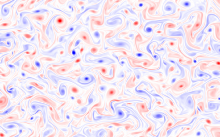
Figure 1: Vorticity $\Omega(x,y)$ in fully developed Hasegawa-Wakatani drift wave turbulence. Negative values are colored in blue, positive values in red. The physical domain is $64\rho_{s}\times 128\rho_{s}$ with a resolution of $n_{x}=512$ and $n_{y}=1024$. The figure is here rotated by 90 degrees for better display. The vortices can often be identified to appear in dipolar pairs.

III 2-D TURBULENCE IN COMPLEX PLASMAS

The motivation for the present contribution originated from discussions during a visit of Padma K. Shukla to University of Innsbruck in 2010. It became clear that a number of problems regarding waves and instabilities in complex plasmas, that Shukla and many other authors had recently addressed by means of linear theory or in 1-d, could often straightforwardly be generalised to a 2-d nonlinear HW like system of fluid equations and put into a form which is directly treatable by our numerical scheme. Shukla had in particular suggested to investigate turbulence in 2-d models for quantum magnetoplasmas, dusty plasmas and strongly coupled fluids. In the following we review the initial results of our simulations.

III.1 Drift wave turbulence in the presence of a dust density gradient

Shukla and Varma Shukla93 have proposed in 1993 a model to study the effect of static, immobile dust grains on waves and instabilities in plasmas. It had been shown that the presence of a static dust density gradient results in modes with a frequency proportional to the dust density gradient scale.

This model has now been cast into a 2-d HW like form that allows the study of drift wave turbulence in the presence of a density gradient of immobile charged dust particles:

$$\partial_{t}n\;+\;[\phi,n] = -(b+a)\;\partial_{y}\phi+D(\phi-n),$$ (5)

$$\partial_{t}\Omega+[\phi,\Omega] = -a\;\partial_{y}\phi-\gamma\;\Omega+D(\phi-n),$$ (6)

where $a=(\epsilon\rho_{d}Z_{d}c/B_{0}n_{i0})\partial_{x}n_{d0}$ with $\epsilon=(+1,-1)$ for (negative, positive) dust, $\rho_{d}=c_{d}/\Omega_{ci}$, where $c_{d}=(\alpha k_{B}T_{e}/m_{i})^{1/2}$ is the modified ion-sound speed Shukla92 with $\alpha=n_{i0}/n_{e0}>1$. The dust related viscosity is given by $\gamma$. The constant plasma density gradient (derived from $N(x)$) is here parametrised by $b=L_{\perp}/L_{n}$, which in our present normalisation is unity. This set of modified HW equations has been derived and numerically solved by Shukla and Kendl in ref. Kendl11-dust . The quasi-linear drift wave instability through an ExB vortex growing out of an initial Gaussian sensity perturbation has been studied for typical resistive drift wave parameters and various dust gradient scales $a$. It has been found that the presence of a co-aligned density gradient of positively charged dust ($a>0$) strongly enhances the resistive drift wave instability, while a counter-aligned dust gradient leads to a damping of the drift waves. The same effect has been seen on fully developed turbulence: co-aligned gradients result in larger fluctuation amplitudes and more pronounced small-scale structures at high $k$, whereas counter-alignment damps the turbulence into quasi-linear modes Kendl11-dust .

The model so far has been restricted on immobile dust grains and did not consider dust charging effects. A comprehensive 2-d multi-species gyrofluid code for a more general modelling of dusty plasma turbulence is presently being developed by the author.

III.2 Generalised (viscoelastic) hydrodynamics

Strongly coupled fluids are often modelled in “generalised hydrodynamics” by including a viscoleastic relaxation time $\tau$ as lowest order manifestation of kinetic coupling effects in the (incompressible) Navier-Stokes equation:

$$(1+\tau\;\partial_{t})\;d_{t}\;\Omega=\sigma\nabla_{\perp}^{2}\Omega$$ (7)

For numerical treatment with our existing solvers we split this equation in two dimensions into the coupled set

$$\partial_{t}\Omega+[\phi,\Omega] = -(1/\tau)(\Omega-\Psi)$$ (8)

$$\partial_{t}\Psi+[\phi,\Omega] = \sigma\nabla_{\perp}^{2}\Omega$$ (9)

so that for $\tau\rightarrow 0$ the Navier-Stokes equation is asymptotically recovered. We have studied vortex stability, propagation and decay with this system. Remarkably, we have found for comparable parameters qualitatively nearly identical results as in a recent study Ashwin11 that employed a “first principles” molecular dynamics code to simulate coherent vortices in strongly coupled liquids.

A personal favourite is the nonlinear evolution of a vortex with just the right relation between initial amplitude and radius (i.e. half-width of a Gaussian). It is well known from classical hydrodynamics that a strong vortex can develop into a rotating tripole and further perform along various routes until decay Fuentes96 .

For certain parameters, the tripole can split up into a dipole pair and a single monopolar vortex. For some parameters the single may just hastily exit the system and leave the pair, which is further waltzing around each other alone.

For other initial parameters, the three can perform a complicated kind of polka, where the separated monopole circles around the rotating dipole in some distance, approaches the pair again to exchange partners, and the freely relased vortex is now circling around the new pair… and so on to viscosity.

A novel aspect regarding this dance, which we now studied with the above set of equations, is the combined effect of viscosity $\sigma$ and viscoelastic relaxation time $\tau$ on this triple polka. We find that by adding high viscosity (e.g. $\sigma=0.1$) the initial vortex may rather (again depending on initial amplitude and scale) disperse outwards and not further develop any nonlinear structures. Adding finite $\tau$ (here in the range between 1 and 10) can compensate for the dispersive action of $\sigma$, and the dipolar or tripolar vortex structures of the inviscid case can be recovered.

III.3 De Broglie screening effect in semi-classical plasmas

Recently, Shukla and Kendl have derived and numerically solved a semi-classical generalisation of the HW equations for dense degenerate Fermi plasmas including quantum pressure corrections Kendl11-QHW . The model is based on the quantum magneto-hydrodynamic model Haas05 ; Brodin07 . The dispersion relation of drift waves in magnetised quantum hydrodynamic plasmas has before been studied by a number of authors in similar linear models, e.g. refs. Shokri99 ; Ali07 .

The semi-classical HW equations in an inhomogeneous magnetic field are Kendl11-QHW :

$$\partial_{t}\Omega+[\phi,\Omega] = D(\phi-\Lambda n)-\kappa(\Lambda^{\!\ast}n)$$ (10)

$$\partial_{t}n\;+\;[\phi,n] = D(\phi-\Lambda n)+\kappa(\phi-\Lambda^{\!\ast}n)$$ (11)

where the curvature operator is defined as

$$\kappa(f)=-c\nabla\times\left({{\bf B}/B^{2}}\right)\cdot\nabla f=-c\nabla\times\left[({\bf B}\times\nabla f)/B^{2}\right].$$

The quantum corrections effect enters through $\Lambda=1-\beta^{2}\nabla^{2}$ and $\Lambda^{\!\ast}=1+\beta^{2}\nabla^{2}$, with $\beta=\lambda_{q}/\rho_{s}$, where $\lambda_{q}=\hbar/\sqrt{4m_{e}T_{F}}$ is the electron de Broglie length and $\rho_{s}$ the drift scale, both here defined at Fermi temperature.

The novel feature of this system is that we find a finite de Broglie length (FBL) screening effect on density fluctuations, which is analogous to the well-known FLR gyro screening and Debye screening of plasma turbulence.

An important caveat concerns the range of validity of the quantum hydrodynamic model. The fluid-like equations including the quantum pressure are derived from the nonlinear Schroedinger equations by means of an eikonal ansatz, replacing the quantum mechanical wave function by an amplitude $n\sim|\Psi|^{2}$, which follows a continuity equation, and a phase function $S$, which dynamically evolves in space and time like a fluid velocity in Euler’s equation. It is important to remember that the eikonal ansatz is valid only in the long wave length regime where all wave lengths $2\pi/k\gg\lambda_{q}$ are required to be much larger than the de Broglie length. This is analogous to the relation between electromagnetic wave optics and geometric ray optics. While this remark may perhaps seem obvious to most readers, it has to be noted that some authors applying quantum plasma hydrodynamic models do unfortunately not seem to be aware of these restrictions.

For quasi-linear drift waves the relevant wave lengths are in the order of a few drift scales $\rho_{s}$, with most unstable modes usually found around $0.1<\rho_{s}k<1$. Choosing the parameter $\beta=\lambda_{q}/\rho_{s}$ well below unity is therefore a safe bet for linear theory. In fully developed turbulence the cascade however in principle reaches down to viscous scales. We do not have a good model of where to properly insert a viscous or Reynolds cut-off in dense quantum plasma turbulence. Cutting the spectrum off by hyperviscosity at scales related to $\rho_{s}/4$ seems tolerable in our experience. In any case we require a small quantum parameter $\beta\ll 1$ for consistency.

In our recent quantum effect studies on resistive drift wave turbulence Kendl11-QHW and interchange modes Kendl11-QIC we have used $\beta=0.5$ as a (perhaps already somewhat questionable) upper limit which is barely consistent with the model validity. The main message here is that our results are highly interesting from an academic point of view, regarding the newly discovered FBL screening effect. From a practical perspective, the quantum parameter in a valid range $\beta\ll 1$ gives only minor corrections to the classical results. When compared to gyrofluids, this limit would somewhat correspond to a Taylor approximation of the gyro-averaging operators – which also is either practically insignificant for most purposes if used in the correct limit, or otherwise simply gives a wrong result.

The validity of quantum hydrodynamics starts to cease at scales just where it is beginning to become interesting. In particular, the important phenomenon of vortex quantisation is not self-consistently treatable at all with the hydrodynamic equations (other than being artifically modelled as specific point or disc vortices).

III.4 Quantum Charney-Obukhov turbulence

The same notes of caution apply to the last quasi-2-d turbulent system, which we here present and have recently addressed numerically. As mentioned in the introduction, there is a well-known isomorphism between the Hasegawa-Mima and Charney-Obukhov models. The latter describes rotating fluids in the presence of a gradient in rotation frequency, which is applicable as a basic model for atmospherical dynamics, and as solution includes Rossby waves and the secondary formation of jet streams. Recent experiments on strongly rotating Bose-Einstein condensates provided a motivation to apply the quantum hydrodynamic approach including strong rotation. A quantum Charney-Obukhov equation has recently been suggested and linearly analysed in ref. Tercas10 :

$$\partial(\nabla^{2}\psi-\phi)-\left[\psi,\phi+\nabla^{2}\psi-\ln N\right]=0$$ (12)

where $\psi=\Lambda\phi$ with $\Lambda=1-\beta^{2}\nabla^{2}$. This equation can be treated with our numerical scheme by explicitly evaluating $\partial W=[\Lambda\phi,\phi+\nabla^{2}\Lambda\phi-\ln N]$, and inverting $W_{k}=(1+k^{2}+(1/2)\beta^{2}k^{4})\phi_{k}$ in Fourier space. We have numerically solved this system by using a Gaussian background rotation $N(r)$ to model a rotating condensate in a trap and initially superimposing a shear flow perturbation at half radius. The shear flow is found to be breaking up into several vortex-like modes rotating around the center of the condensate (see figure 2), and then is rather rapidly decaying, when the shear flow perturbation is not continously driven.

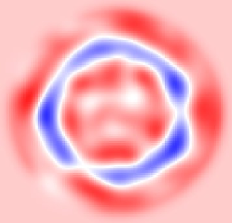
Figure 2: A shear flow perturbation is superimposed on a circular rotating quantum fluid in a 2-d numerical solution of the (actually semi-classical) quantum Charney-Obukhov model. Here the perturbed stream function $\phi(x,y)$ is shown, which develops a modal structure and (depending on parameters, here $\beta=0.8$) either rapidly decays or transiently forms a chain of rotating vortices. Note the absence of vortex quantisation in this simplified model. The color coding is blue for positive (corresponding to the initial perturbation) and red for negative values of $\phi$. Stream lines of the fluid flow are on isocontours of the stream function.

To the best of our knowledge, such a nonlinear 2-d quantum hydrodynamical model of rapidly rotating Bose-Einstein condensates has not been simulated before. But again, in the valid range the small quantum factor $\beta$ does not produce any significant effects. The behaviour of the system is found to be very similar to a classical rotating fluid.

What of course is completely absent in this model is vortex quantisation. And as this is just the whole crux of quantum turbulence, the hydrodynamic approach on BECs can in the personal opinion of the author be regarded as rather useless. Nothing new is learned, much is lost. There seems to be no good reason for not rather solving the GPE (which is really rather standard now) to model BECs.

IV CONCLUSIONS

We have numerically studied the formation and evolution of nonlinear and turbulent dynamical structures in two-dimensional complex plasmas and fluids. Generalised (drift) fluid simulations have been developed on the basis of the Hasegawa-Wakatani model and the 2-d Navier-Stokes vorticity equation.

Recently published results on turbulence in dusty magnetised plasmas and semi-classical (“quantum”) plasmas have been reviewed.

New results on 2-d generalised hydrodynamics including viscoelastic relaxation effects were presented. The first nonlinear quantum hydrodynamic simulation of a rotating Bose-Einstein condensate has been presented. The limits of validity of the quantum hydrodynamic model with respect to turbulence was critically discussed.

References

- (1) M. Bonitz, Introduction to Complex Plasmas (Springer Series on Atomic, Optical, and Plasma Physics). Springer Berlin Heidelberg, 2010.
- (2) V.E. Fortov, G.E. Morfill, Complex and Dusty Plasmas: From Laboratory to Space. CRC Press, 2009.
- (3) T.C. Killian, Science 316, 705-708 (2007).
- (4) S.L. Rolston, Physics 1, 2 (2008).
- (5) A. Kendl, Plasma turbulence in complex magnetic field structures. Innsbruck University Press, 2007.
- (6) A. Hasegawa, M. Wakatani, Phys. Rev. Lett. 50, 682 (1983).
- (7) A.J. Brizard, T.S. Hahm, Rev. Mod. Phys, 79, 421 (2007).
- (8) A.E. Koniges, J.A. Crotinger, P.H, Diamond, Phys. Fluids B 4, 2785 (1992),
- (9) D. Biskamp, S.J. Camargo, B.D. Scott, Phys. Lett. A 186, 239 (1994).
- (10) S.J. Camargo, D. Biskamp, B.D. Scott, Phys. Plasmas 2, 48 (1995)
- (11) T.S. Pedersen, P.K. Michelsen, J.J. Rasmussen, Phys. Plasmas 3, 2939 (1996).
- (12) A. Zeiler, D. Biskamp, J.F. Drake, Phys. Plasmas 3, 3947 (1996).
- (13) G.Z. Hu, J.A. Krommes, J.C. Bowman, Phys. Plasmas 4, 2116 (1997).
- (14) S.B. Korsholm, P.K. Michelsen PK, V. Naulin, Phys. Plasmas 6, 2401 (1999).
- (15) M. Priego, O.E. Garcia, V. Naulin, J.J. Rasmussen, Phys. Plasmas 12, 062312 (2005).
- (16) R. Numata, R. Ball, R.L. Dewar, Phys. Plasmas 14, 102312 (2007).
- (17) C. Holland, G. Tynan, J. James, et al. Plasma Phys. Control. Fusion 49, A109 (2007).
- (18) A. Kendl, Phys. Plasmas 18, 072303 (2011).
- (19) A. Hasegawa, K. Mima, Phys. Rev. Lett. 39, 205 (1977).
- (20) W. Horton, A. Hasegawa, Chaos 4, 227 (1994).
- (21) P.H. Diamond, S.-I. Itoh, K. Itoh, T.S. Hahm, Plasma Phys. Control. Fusion 47, R35 (2005).
- (22) G.E. Karniadakis, M. Israeli, S.A. Orszag, J. Comput. Phys. 97, 414 (1991).
- (23) A. Arakawa, J. Comput. Phys. 1, 119 (1966).
- (24) V. Naulin, A. Nielsen, SIAM J. Sci Comput. 25, 104 (2003).
- (25) B.D. Scott, New J. Phys. 7, 92 (2005).
- (26) P.K. Shukla, R.K. Varma, Phys. Fluids 5, 236 (1993).
- (27) P.K. Shukla and V.P. Silin, Phys. Scr. 45, 508 (1992).
- (28) A. Kendl, P.K. Shukla, submitted to Phys. Rev. E (2011).
- (29) J. Ashwin, R. Ganesh, Phys. Rev. Lett. 106, 135001 (2011).
- (30) O.U. Velasco Fuentes, G.J.F. van Heijst, N.P.M. van Lipzig, Journal of Fluid Mechanics 307, 11-41 (1996).
- (31) A. Kendl, P.K. Shukla, Phys. Lett. A 375, 3138 (2011).
- (32) F. Haas, Phys. Plasmas 12, 062117 (2005).
- (33) G. Brodin and M. Marklund, Phys. Plasmas 14, 112107 (2007); New J. Phys. 9, 227 (2007); M. Marklund and G. Brodin, Phys. Rev. Lett. 98, 025001 (2007).
- (34) B. Shokri and A. Rukhadze, Phys. Plasmas 6, 4467 (1999).
- (35) S. Ali et al., Eur. Phys. Lett. 78, 45001 (2007).
- (36) A. Kendl, submitted to Phys. Rev. E (2011).
- (37) H. Tercas, J.P.A. Martins, J.T. Mendonca, New J. Phys. 12, 093001 (2010).