Tailoring population inversion in Landau-Zener-Stückelberg interferometry of flux qubits

Abstract

We distinguish different mechanisms for population inversion in flux qubits driven by dc+ac magnetic fields. We show that for driving amplitudes such that there are Landau-Zener-Stückelberg interferences, it is possible to have population inversion solely mediated by the environmental bath. Furthermore, we find that the degree of population inversion can be controlled by tailoring a resonant frequency $\Omega_{p}$ in the environmental bath. To observe these effects experiments should be performed for long driving times after full relaxation.

Population inversion, where the most highly populated state is an excited state, is among the most interesting phenomena in maser and laser physics lasers . The usual mechanism to get population inversion (PI) requires driven quantum systems with three or more energy levels lasers ; lukens ; nori2007 ; astafiev . Interesting systems to study PI are ‘artificial atoms’ made with mesoscopic Josephson devices revqubits ; nori2011 . Among them, a well known circuit is the flux qubit (FQ) qbit_mooij ; chiorescu . When driven by a dc+ac magnetic flux, it has transitions between energy levels at avoided crossings. A rich structure of Landau-Zener-Stückelberg (LZS) interferences shevchenko combined with multi-photon resonances oliver ; valenzuela ; izmalkov is observed. LZS interference patterns have also been measured in charge qubits cqubits , Rydberg atoms yoakum , ultracold molecular gases mark , optical lattices kling and single electron spins huang . In FQ, diamond-like patterns were found for large ac amplitudes, from which the energy level spectrum has been reconstructed valenzuela . Population inversion was observed in the ‘second diamond’, i. e. for ac amplitudes that excite to the third and four energy levels through Landau-Zener transitions. PI was also measured in another flux qubit device driven at large frequencies sun . Here we will show that an even more notable effect is awaiting to be observed in these systems if the ac driving pulses are applied for longer time scales: PI could be observable even for ac amplitudes where only the two lowest levels of the FQ participate. In the following we will explain, through realistic time-dependent numerical simulations, (i) how this type of PI can occur, (ii) why it has not been observed experimentally yet and (iii) how the occurrence and the degree of PI can be tailored by changing the structure of the environmental bath.

The FQ consists of a superconducting ring with three Josephson junctions qbit_mooij enclosing a magnetic flux $\Phi=f\Phi_{0}$ ($\Phi_{0}=h/2e$) with phase differences $\varphi_{1}$, $\varphi_{2}$ and $\varphi_{3}=-\varphi_{1}+\varphi_{2}-2\pi f$. Two of the junctions have coupling energy, $E_{J}$, and capacitance, $C$, and the other has $E_{J,3}=\alpha E_{J}$ and $C_{3}=\alpha C$. The hamiltonian is: qbit_mooij

$${\cal H}=-2E_{C}\left(\frac{\partial^{2}}{\partial\varphi_{t}^{2}}+\frac{1}{1+2\alpha}\frac{\partial^{2}}{\partial\varphi_{l}^{2}}\right)+E_{J}V(\varphi_{t},\varphi_{l})\;,$$ (1)

with $\varphi_{t}=(\varphi_{1}+\varphi_{2})/2$, $\varphi_{l}=(\varphi_{1}-\varphi_{2})/2$, $E_{C}=e^{2}/2C$ and $V(\varphi_{t},\varphi_{l})=2+\alpha-2\cos\varphi_{t}\cos\varphi_{l}-\alpha\cos(2\pi f+2\varphi_{l})$. The FQ has several discrete levels with eigenenergies $E_{i}$ and eigenstates $|\Psi_{i}\rangle$ which depend on $f$, $\alpha$ and $\eta=\sqrt{8E_{C}/E_{J}}$. Typical experiments have $\alpha\sim 0.6-0.9$ and $\eta\sim 0.1-0.6$ chiorescu ; oliver ; valenzuela . For $\alpha\geq 1/2$ and $|f-1/2|\ll 1$, the potential $V(\varphi_{t},\varphi_{l})$ has the shape of a double-well with two minima along the $\varphi_{l}$ direction. In this regime the system can be operated as a quantum bit qbit_mooij ; chiorescu and approximated by a two-level system (TLS) qbit_mooij ; ferron . When driven by a magnetic flux $f(t)=f_{dc}+f_{ac}\sin(\omega t)$, the hamiltonian is time periodic ${\cal H}(t)={\cal H}(t+\tau)$, with $\tau=2\pi/\omega$. In the Floquet formalism, which allows to treat periodic forces of arbitrary strength and frequency floquet ; fds , the solutions of the Schrödinger equation are of the form $|\Psi_{\beta}(t)\rangle=e^{i\varepsilon_{\beta}t/\hbar}|\Phi_{\beta}(t)\rangle$, where the Floquet states $|\Phi_{\beta}(t)\rangle$ satisfy $|\Phi_{\beta}(t)\rangle$=$|\Phi_{\beta}(t+\tau)\rangle=\sum_{k}|\Phi_{\beta}^{k}\rangle e^{-ik\omega t}$, and are eigenstates of the equation $[{\cal H}(t)-i\hbar\partial/\partial t]|\Phi_{\beta}(t)\rangle=\varepsilon_{\beta}|\Phi_{\beta}(t)\rangle$, with $\varepsilon_{\beta}$ the associated quasi-energy.

Experimentally, the system is affected by the electromagnetic environment that introduces decoherence and relaxation processes. A standard theoretical model is to linearly couple the system to a bath of harmonic oscillators hanggi ; milenas ; grifonih ; caspar with a spectral density $J(\omega)$ and equilibrated at temperature $T$. For the FQ, the dominating source of decoherence is flux noise, in which case the bath degrees of freedom couple with the system variable $\varphi_{l}$ (see caspar ). For weak coupling (Born approximation) and fast bath relaxation (Markov approximation), a Floquet-Born-Markov master equation for the reduced density matrix $\hat{\rho}$ in the Floquet basis, $\rho_{\alpha\beta}(t)=\langle\Phi_{\alpha}(t)|\hat{\rho}(t)|\Phi_{\beta}(t)\rangle$, can be obtained hanggi :

$$\frac{d\rho_{\alpha\beta}(t)}{dt}=-\frac{i}{\hbar}(\varepsilon_{\alpha}-\varepsilon_{\beta})\rho_{\alpha\beta}(t)+\sum_{\alpha^{\prime}\beta^{\prime}}{\it L}_{\alpha^{\prime}\beta^{\prime}\alpha\beta}(t)\;\rho_{\alpha^{\prime}\beta^{\prime}}(t)\;.$$ (2)

The ${\it L}_{\alpha^{\prime}\beta^{\prime}\alpha\beta}(t)$ are approximated by their average over one period $\tau$ hanggi since the time scale $t_{r}$ for full relaxation satisfies $t_{r}\gg\tau$, obtaining ${\it L}_{\alpha^{\prime}\beta^{\prime}\alpha\beta}=R_{\alpha^{\prime}\beta^{\prime}\alpha\beta}+R_{\beta^{\prime}\alpha^{\prime}\beta\alpha}^{*}-\sum_{\eta}\left(\delta_{\beta\beta^{\prime}}R_{\alpha^{\prime}\alpha\eta\eta}+\delta_{\alpha\alpha^{\prime}}R_{\beta^{\prime}\beta\eta\eta}^{*}\right)$. The rates $R_{\alpha^{\prime}\beta^{\prime}\alpha\beta}=\sum_{n}g_{\alpha\alpha^{\prime}}^{n}\Gamma_{\alpha\alpha^{\prime}}^{n}\Gamma_{\beta^{\prime}\beta}^{-n}$ are sums of $n$-photon exchange terms, with $g_{\alpha\alpha^{\prime}}^{n}=J(\frac{\varepsilon_{\alpha\alpha^{\prime}}^{n}}{\hbar})\left(\coth(\frac{\varepsilon_{\alpha\alpha^{\prime}}^{n}}{2k_{B}T})-1\right)$, $\varepsilon_{\alpha\alpha^{\prime}}^{n}=\varepsilon_{\alpha}-\varepsilon_{\alpha^{\prime}}+n\hbar\omega$, and $\Gamma_{\alpha\alpha^{\prime}}^{n}=\sum_{k}\langle\Phi_{\alpha}^{k}|\varphi_{l}|\Phi_{\alpha^{\prime}}^{k+n}\rangle$. This formalism has been extensively employed to study relaxation and decoherence for time dependent periodic evolutions in double-well potentials and in TLS hanggi ; milenas ; grifonih . Here we use it to model the ac driven FQ for the full hamiltonian of Eq. (1), beyond the TLS approximation. We calculate the Floquet states $|\Phi_{\beta}^{k}\rangle$ and quasienergies $\varepsilon_{\beta}$ fds , and then we integrate numerically Eq. (2), obtaining $\rho_{\alpha\beta}(t)$ as a function of $t$.

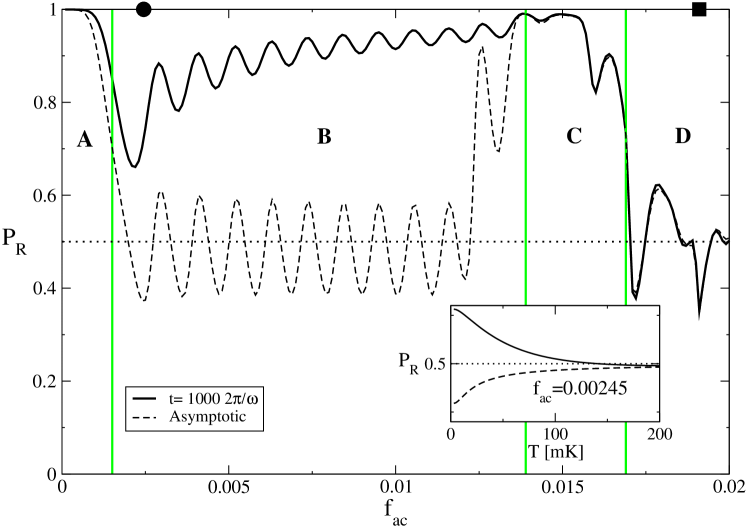
Figure 1: Population $P_{R}$ as a function of the driving amplitude $f_{ac}$. Continuous line: $P_{R}(t=1000\tau\sim t_{\rm exp})$. Dashed line: asymptotic average population $\overline{P}_{R}$. Inset: $P_{R}$ vs. $T$ for a driving amplitude $f_{ac}=0.00245$. The calculations were performed for $f_{dc}=0.50151$, $\omega=0.003E_{J}/\hbar$ and an ohmic bath with $\gamma=0.001$ at $T=20\rm{mK}$ (for $E_{J}/h\approx 300{\rm GHz}$). Vertical lines separate regimes A, B, C, D described in the text. Black circle: $f_{ac}$ corresponding to the inset, Fig.2(a) and Fig.3. Black square: $f_{ac}$ corresponding to Fig.2(b).

We start by considering a FQ coupled to a bath with an ohmic spectral density $J(\omega)=\gamma\omega$. We take $\gamma=0.001$, corresponding to weak dissipation as in valenzuela , and the bath at $T=0.0014E_{J}/k_{B}$ ($\sim 20{\rm mK}$ for $E_{J}/h\sim 300{\rm GHz}$). The FQ device parameters are $\alpha=0.8$ and $\eta=0.25$. The static field is taken as $f_{dc}=0.50151$, and for the driving microwave field we choose $\omega=0.003E_{J}/\hbar\sim 900\rm{MHz}$ and different amplitudes $f_{ac}$. The initial condition is the ground state $|\Psi_{0}\rangle$ of the static hamiltonian $H_{0}\equiv{\cal H}(f_{dc})$.

Experimentally, the probability of having a state of positive or negative persistent current in the FQ is measured chiorescu . The probability of a positive current measurement (“right” side of the double-well potential) can be calculated as $P_{R}(t)={\rm Tr}(\hat{\Pi}_{R}\hat{\rho}(t))$, with $\hat{\Pi}_{R}$ the operator that projects wave functions on the $\varphi_{l}>0$ subspace fds . For a static field $f_{dc}\gtrsim 1/2$, the ground state has $P_{R}\approx 1$. In Fig.1 we show, as a function of $f_{ac}$, $P_{R}(t)$ after a driving time $t=1000\tau$, which is similar to the time scale $t_{\rm exp}$ of the experiments valenzuela . We also plot the asymptotic ${\overline{P}_{R}}\equiv{\rm lim}_{t\rightarrow\infty}\langle P_{R}(t)\rangle_{\tau}$, averaged over one period $\tau$. We find different regimes: (A) For small $f_{ac}$, $P_{R}\sim 1$, since the system is slightly perturbed from the ground state. (B) When further increasing $f_{ac}$, new regimes are found whenever the extreme driving amplitudes $f_{dc}\pm f_{ac}$ reach an avoided crossing in the energy level spectrum $\{E_{i}(f))\}$. Since the slopes $\frac{-dE_{i}}{df}$ are proportional to the average loop current of the FQ, at avoided crossings there is interference between “positive” and “negative” loop current states, which results in LZS oscillations shevchenko in the dependence of $P_{R}$ with $f_{ac}$. The first case is found when the avoided crossing at $f=1/2$ between the ground state level $E_{0}$ and the first excited level $E_{1}$ is reached, and the transfer of population to the $E_{1}$ level lowers $P_{R}$. The FQ of oliver ; valenzuela has a decoherence time $t_{\phi}\sim 20{\rm ns}>\tau$ and a large ‘interwell‘ relaxation time $t_{r}\sim 100\mu{\rm s}$. Due to this time scale separation ($t_{\phi}<t_{\rm exp}\ll t_{r}$), a TLS model with classical noise, valid for $t<t_{r}$, can explain the experimentally observed LZS oscillations of $P_{R}$ vs. $f_{ac}$, where the minima correlate with the zeros of Bessel functions $J_{n}(af_{ac}/\omega)$ ($a$ a normalization constant) oliver ; shevchenko . The results of Fig.1 for $t=1000\tau\sim t_{\rm exp}$ are in agreement with this finding. However, the finite time $P_{R}(t_{\rm exp})$ is very different from the asymptotic ${\overline{P}_{R}}$, that even shows population inversion, ${\overline{P}_{R}}<1/2$. (C) At higher values of $f_{ac}$ the avoided level crossing between $E_{1}$ and $E_{2}$ is reached and the ground level $E_{0}$ is repopulated due to fast $E_{2}\rightarrow E_{0}$ ‘intrawell’ transitions (the corresponding states have the same sign of the average loop current). Thus, $P_{R}$ increases close to $1$ (‘cooling’ effect, see valenzuela ). When more than two levels are involved, ‘intrawell’ relaxation in a time scale $t_{i}$ is possible. In the experiments, $t_{i}\sim 50{\rm ns}\ll t_{r}$ valenzuela . This explains that $P_{R}(t_{\rm exp})\approx{\overline{P}_{R}}$, since intrawell processes dominate relaxation to the asymptotic state and $t_{i}<t_{\rm exp}$. (D) For $f_{ac}$ such that the symmetrically located (with respect to $f=1/2$) avoided crossing between $E_{1}$ and $E_{2}$ is reached, there are new LZS oscillations. Furthermore the levels $E_{0}$ and $E_{3}$ are also involved in the dynamics (since the avoided crossings between $E_{2}\leftrightarrow E_{3}$ and $E_{0}\leftrightarrow E_{1}$ are traversed by the driving) and a more complex dependence of $P_{R}$ with $f_{ac}$ emerges. In this case, we find population inversion, which is also observed experimentally in valenzuela . A multilevel extension of the semiclassical model of oliver can describe this behavior as well wen .

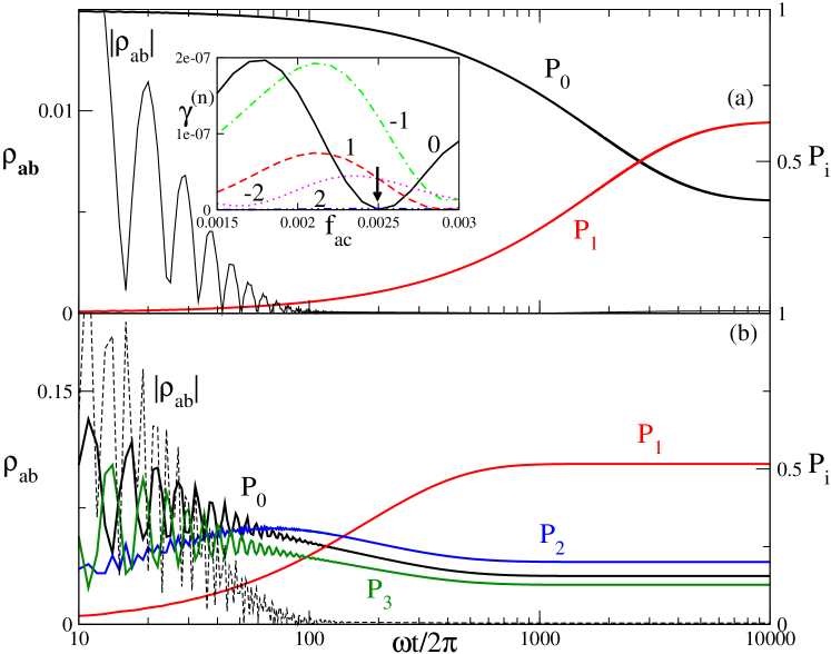
Figure 2: (color online) Off-diagonal (in Floquet basis) density matrix element $\rho_{ab}$ (left axis) and level population $P_{i}$ (right axis) as a function of time (log) for $f_{dc}=0.50151$, $\omega=0.003E_{J}/\hbar$, $\gamma=0.001$. (a) $f_{ac}=0.00245$ and (b) $f_{ac}=0.0191$. Inset: $n$-photon relaxation terms $\gamma^{(n)}$ (the corresponding $n$ value is indicated on the top of each curve) in the neighborhood of $f_{ac}=0.00245$ (indicated by the arrow).

In Fig.2 we show the explicit time dependence of $\rho_{\alpha\beta}(t)$ for two values of $f_{ac}$ in regimes (B) and (D) respectively. The off-diagonal elements $\rho_{\alpha\beta}$ decay exponentially to zero in a time scale $t_{\phi}$ [see Fig.2(a) and (b), left axis]. In the Floquet basis, after full decoherence, the relaxation process is determined by the evolution of the diagonal $\rho_{\alpha\alpha}(t)$ for $t>t_{\phi}$ comment . Thus the asymptotic regime can be obtained from the non-trivial solution of $\sum_{\beta}L_{\beta\beta,\alpha\alpha}\,\rho_{\beta\beta}=0$ after imposing $\frac{d\rho_{\alpha\alpha}}{dt}=0$ in Eq.(2). In this way, we calculated the ${\overline{P}_{R}}$ shown in Fig.1 as a function of $f_{ac}$. In order to understand the emergence of population inversion in the asymptotic limit, we evaluate the population of the eigenstates of $H_{0}$, $P_{i}(t)=\langle\Psi_{i}|\hat{\rho}(t)|\Psi_{i}\rangle$. We distinguish two mechanisms of PI:

(i) Third-level-mediated population inversion: For large $f_{ac}$ [regime (D) in Fig.1], the populations $P_{i}$ relax to the asymptotic regime in a short time scale similar to $t_{i}\gtrsim t_{\phi}$. In Fig.2(b) we see that the populations $P_{2},P_{3}$ start increasing, and later they decrease transferring population to $P_{1}$. This leads to population inversion, $P_{1}>P_{0}$, mediated by $E_{2}$ and $E_{3}$, which is the usual mechanism for this effect. In our case the higher levels are reached through LZS transitionsvalenzuela ; wen instead of resonant transitions.

(ii) Bath-mediated population inversion:

In Fig.2(a) we show results for a value of $f_{ac}=0.00245$ such that only LZS interference between the two lowest energy levels occurs [regime (B) in Fig.1]. Thus one can restrict to two Floquet states $\alpha=a,b$. We find that the decay time $t_{\phi}$ of the off-diagonal $\rho_{ab}$ is similar to the previous case but the level populations relax to their asymptotic value in a very large time scale $t_{r}\gg t_{\phi}$. Only for $t\gtrsim t_{r}$ population inversion can arise. The large $t_{r}$ explains the difference between ${\overline{P}_{R}}$ and the finite time $P_{R}(t\sim t_{\rm exp})$ in Fig.1. To understand the underlying mechanism we decompose the relaxation rate $\gamma_{r}={t_{r}}^{-1}$ as $\gamma_{r}=2(R_{aabb}+R_{bbaa})=\gamma^{(0)}+\sum_{n\not=0}\gamma^{(n)}$, with $\gamma^{(n)}=2(g_{ab}^{n}|\Gamma_{ab}^{n}|^{2}+g_{ba}^{n}|\Gamma_{ba}^{n}|^{2})$ the terms that describe virtual n-photon transitions to bath oscillator states grifonih . In the inset of Fig.2(a) we show that when there is PI the term $\gamma^{(n=-1)}$ is the largest while $\gamma^{(n=0)}\approx 0$. This indicates that the dominant mechanisms leading to PI is a transition to a virtual level at energy $E_{0}+\hbar\omega>E_{1}$ (one photon absorption, $n=-1$), followed by a relaxation to $E_{1}$. Previous works have found PI, under various approximations, but for the asymptotic regime of TLS popin2l ; hartmann ; stace2005 ; yu2010a . However the time-dependent dynamics with different time scales has been overlooked. In fact, the relevant point from our findings is that the asymptotic regime is difficult to reach in the experiment, since PI needs long times ($t\gtrsim t_{r}\gg t_{\phi}$) to emerge when mediated by the bath. Moreover, the difference between $P_{R}(t_{\rm exp})$ and the asymptotic $\overline{P}_{R}$, is enhanced when decreasing temperature (see inset of Fig.1)

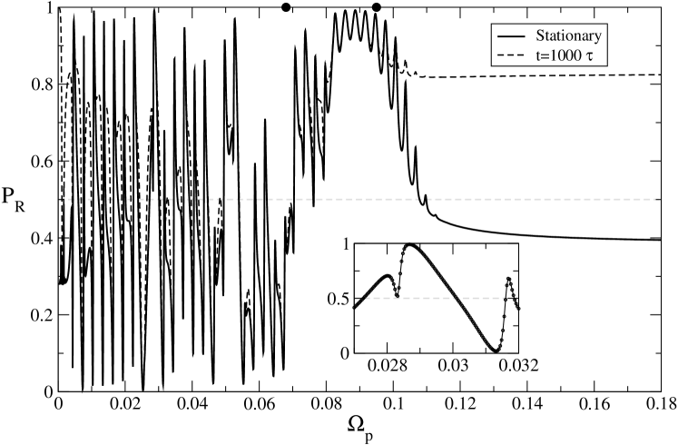
Figure 3: Population $P_{R}$ as a function of the frequency $\Omega_{p}$ (in units of $E_{J}/\hbar$) for $T=20{\rm mK}$, $f_{dc}=0.50151$, $f_{ac}=0.00245$, $\omega=0.003E_{J}/\hbar$, $\gamma=0.001$ and $\kappa=0.001$. Continuous line shows the asymptotic $\overline{P}_{R}$ and dashed line corresponds to $P_{R}(t=1000\tau\sim t_{\rm exp})$. The circles indicate the values of $\Delta_{+}$ and $\Delta_{-}$. The inset shows $\overline{P}_{R}$ as a function of $\Omega_{p}$ around the $n=9$ resonance. See text for details.

An interesting consequence of the ‘bath-mediated’ mechanism is that it enables - by changing the spectral structure of the bath - to modify the asymptotic state of the FQ. In particular, a realistic modeling of the environmental bath for FQ includes a read-out dc SQUID inductively coupled to the FQ qbit_mooij ; caspar ; chiorescu2 . For this case, the bath spectral density becomes $J_{sb}(\omega)={\gamma\omega\Omega_{p}^{4}}/[(\Omega_{p}^{2}-\omega^{2})^{2}+(2\pi\kappa\omega\Omega_{p})^{2}]$, with $\Omega_{p}$ the resonant frequency of the SQUID detector, and $2\pi\kappa\Omega_{p}$ the width of the resonance at $\omega=\Omega_{p}$ caspar . In Fig.3 we show ${\overline{P}_{R}}$ as a function of $\Omega_{p}$ for the same $f_{ac}$ of Fig.2(a), but after solving Eq.(2) with $J_{sb}(\omega)$. We identify three regimes in the overall behavior of ${\overline{P}_{R}}$ vs $\Omega_{p}$ that we describe below. Defining $\Delta(f)=E_{1}(f)-E_{0}(f)$, $\Delta_{+}=\Delta(f_{dc}+f_{ac})$ and $\Delta_{-}=\Delta(f_{dc}-f_{ac})$ we get: (1) Multiphoton resonances with the bath. For $\Omega_{p}<\Delta_{-}$ the population ${\overline{P}_{R}}$ has a strong dependence on $\Omega_{p}$, displaying resonances for $\Omega_{p}\approx n\omega+\varepsilon_{b}-\varepsilon_{a}$ (with $\varepsilon_{b},\varepsilon_{a}$ the quasienergies of the Floquet states mostly weighted in the two lowest $H_{0}$ eigenstates). These resonances correspond to the maxima at $\Omega_{p}$ of the $J_{sb}(\varepsilon_{a}-\varepsilon_{b}+n\hbar\omega)$, and have been previously discussed for $n=1$ within a perturbative approach milenas . Near these resonances it is possible to fully control the population ${\overline{P}_{R}}$, going from ${\overline{P}_{R}}\sim 1$ to complete population inversion ${\overline{P}_{R}}\sim 0$, with small changes of $\Omega_{p}$. In the inset of Fig.3 we show in detail the case near the $n=9$ resonance. (2) Bath mediated population inversion. In the opposite limit, $\Omega_{p}>\Delta_{+}$, the behavior is similar to the one discussed previously in Fig.2(a), since for large $\Omega_{p}$, the spectral density $J_{sb}(\omega)\rightarrow\gamma\omega$ (3) Bath mediated cooling. In the intermediate regime, $\Delta_{-}\lesssim\Omega_{p}\lesssim\Delta_{+}$, transitions to an effective energy level milenas ; chiorescu2 at $E_{0}+\Omega_{p}<E_{1}$ predominate. From this effective level it is possible to decay and repopulate the ground state, obtaining ${\overline{P}_{R}}\sim 1$. The resonances at $\Omega_{p}\approx n\omega+\varepsilon_{b}-\varepsilon_{a}$ are still observed. A full picture of the effect of a structured bath can be observed in Fig.4, which shows a map of the asymptotic population ${\overline{P}_{R}}$ as a function of $\Omega_{p}$ and $f_{ac}$. The onset of third level mediated PI at higher $f_{ac}$ (corresponding to the second ’diamond’ of valenzuela ) is also observed. Notice that this type of PI is almost independent of $\Omega_{p}$, while the bath-mediated mechanism is active for $\Omega_{p}>\Delta_{+}$.

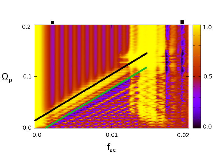
Figure 4: (color online) Contour map of the asymptotic population $\overline{P}_{R}$ as a function of the driving amplitude $f_{ac}$ and the resonance frequency $\Omega_{p}$ (in units of $E_{J}/\hbar$) for $T=20{\rm mK}$, $f_{dc}=0.50151$, $\omega=0.003E_{J}/\hbar$, $\gamma=0.001$ and $\kappa=0.001$. The black and green lines represent the positions of $\Delta_{+}$ and $\Delta_{-}$. Black circle: $f_{ac}$ corresponding to Fig.2(a) and Fig.3; black square: $f_{ac}$ corresponding to Fig.2(b).

In conclusion, by performing a realistic modeling of the FQ we are able to analyse different scenarios for population inversion in strongly driven quantum systems, understanding the parameter regimes for their occurrence. One puzzling situation is that the bath-mediated PI discussed here has not been observed in valenzuela . The large time scale separation $t_{r}\gg t_{\phi}$ in the device of valenzuela suggests that the PI could be beyond the experimental time window comment3 . Indeed, our results explain that to observe this effect the experiments should be carried out for long driving times, after full relaxation with the bath degrees of freedom ($t\gtrsim t_{r}$). A remarkable point we found is the dependence of the LZS oscillations on the frequency $\Omega_{p}$ of the SQUID detector. The FQ fabricated with Nb junctions as in oliver ; valenzuela have typically a small gap and thus they are in the regime $\Omega_{p}>\Delta_{+}$, where bath-mediated PI can take place. The FQ fabricated with Al junctions, as in chiorescu ; chiorescu2 , have a large gap and thus they are expected to be in the regime $\Omega_{p}<\Delta_{-}$. Amplitude spectroscopy measurements carried out in these later systems could give different ‘diamond’ patterns as a function of $f_{dc},f_{ac}$ with resonances and LZS interference effects from the oscillator levels at $E_{i}+n\hbar\Omega_{p}$. In principle, the frequency $\Omega_{p}$ can be controlled by varying in the SQUID detector the driving current or the shunt capacitor chiorescu2 , or by adding a tunable resonator to the circuit deppe . In these cases there is room to fully tailor the population $P_{R}$. Furthermore, the discussed population inversion scenarios could also apply to other quantum systems in which LZS interference has been measured cqubits ; yoakum ; mark ; kling ; huang .

We acknowledge discussions with Sergio Valenzuela and financial support from CNEA, CONICET (PIP11220080101821 and PIP11220090100051) and ANPCyT (PICT2006-483 and PICT2007-824).

References

- (1) J. Weber, Rev. Mod. Phys. 31, 681 (1959)
- (2) S. Y. Han, R. Rouse, and J. E. Lukens, Phys. Rev. Lett. 76, 3404 (1996).
- (3) J. Q. You et al, Phys. Rev. B 75, 104516 (2007).
- (4) O. Astafiev et al, Nature 449, 588 (2007).
- (5) Y. Makhlin, G. Schön, and A. Shnirman, Rev. Mod. Phys. 73, 357 (2001).
- (6) J. Q. You and F. Nori, Nature 474, 589 (2011).
- (7) T.P.Orlando et al, Phys. Rev. B 60, 15398 (1999).
- (8) I. Chiorescu et al, Science 299, 1869 (2003).
- (9) S.N. Shevchenko, S. Ashhab and Franco Nori, Phys. Rep. 492, 1 (2010).
- (10) W. D. Oliver et al, Science 310, 1653 (2005); D. M. Berns et al, Phys. Rev. Lett. 97, 150502 (2006).
- (11) D. M. Berns et al, Nature 455, 51 (2008); W D. Oliver and S. O. Valenzuela, Quantum Inf. Process 8, 261 (2009).
- (12) A. Izmalkov et al, Phys. Rev. Lett. 101, 017003 (2008).
- (13) Y. Nakamura, Yu. A. Pashkin, and J. S. Tsai, Phys. Rev. Lett. 87, 246601 (2001); M. Sillanpaa et al, Phys. Rev. Lett. 96, 187002 (2006). C. M. Wilson et al, Phys. Rev. Lett. 98, 257003 (2007).
- (14) S. Yoakum et al, Phys. Rev. Lett. 69, 1919 (1992).
- (15) M. Mark et al, Phys. Rev. Lett. 99, 113201 (2007).
- (16) S. Kling et al, Phys. Rev. Lett. 105, 215301 (2010)
- (17) P.Huang et al, Phys. Rev. X 1, 011003 (2011).
- (18) G. Z. Sun et al, Appl. Phys. Lett. 94, 102502 (2009);
- (19) A. Ferrón and D. Dominguez, Phys. Rev. B 81, 104505 (2010).
- (20) J. H. Shirley, Phys. Rev. 138, B979 (1965).
- (21) A. Ferrón, D. Domínguez and M. J. Sánchez, Phys. Rev. B. 82,134522 (2010).
- (22) S. Kohler et al, Phys. Rev. E. 58, 7219 (1998), H.-P. Breuer, W. Huber and F. Petruccione, Phys. Rev. E 61, 4883 (2000); D. W. Hone, R. Ketzmerick and W. Kohn, Phys. Rev. E 79, 051129 (2009).
- (23) M. C. Goorden, M. Thorwart and M. Grifoni, Phys. Rev. Lett. 93, 267005 (2004); Eur. Phys. J. B 45, 405 (2005).
- (24) J. Hausinger and M. Grifoni, Phys. Rev. A 81, 022117 (2010).
- (25) C. H. van der Wal et al, Eur. Phys. J. B 31, 111 (2003); G. Burkard, R. H. Koch, and D. P. DiVincenzo, Phys. Rev. B 69, 064503 (2004).
- (26) X. Wen and Y. Yu, Phys. Rev. B. 79, 094529 (2009).
- (27) This is expected for , which is fulfilled for very weak coupling with the environment, see hanggi .
- (28) Yu. Dakhnovskii and R.D. Coalson, J. Chem. Phys. 103, 2908 (1995); I.A. Goychuk, E.G. Petrov, and V. May, Chem. Phys. Lett. 253, 428 (1996).
- (29) L. Hartmann et al, Phys. Rev. E 61, R4687 (2000).
- (30) T.M. Stace, A. C. Doherty, and S. D. Barrett, Phys. Rev. Lett. 95, 106801 (2005).
- (31) L. Du, M. Wang, Y. Yu., Phys. Rev. B 82, 045128 (2010).
- (32) I. Chiorescu et al., Nature (London) 431, 159 (2004); J. Johansson et al, Phys. Rev. Lett. 96, 127006 (2006)
- (33) Moreover, in valenzuela is much larger than for the parameters used here, where for numerical convenience we have chosen a larger gap and a larger .
- (34) F. Deppe et al, Nature Physics 4, 686(2008); A. Fedorov et al, Phys. Rev. Lett. 105, 060503 (2010).