Zhongkui Li, Xiangdong Liu, Mengyin Fu, Lihua Xie

Abstract: This paper addresses the global consensus problems of a class of nonlinear multi-agent systems with Lipschitz nonlinearity and directed communication graphs, by using a distributed consensus protocol based on the relative states of neighboring agents. A two-step algorithm is presented to construct a protocol, under which a Lipschitz multi-agent system without disturbances can reach global consensus for a strongly connected directed communication graph. Another algorithm is then given to design a protocol which can achieve global consensus with a guaranteed $H_{\infty}$ performance for a Lipschitz multi-agent system subject to external disturbances. The case with a leader-follower communication graph is also discussed. Finally, the effectiveness of the theoretical results is demonstrated through a network of single-link manipulators.

Keywords: Multi-agent system, global consensus, Lipschitz nonlinearity, $H_{\infty}$ control.

1 Introduction

In recent years, consensus control of multi-agent systems has been an emerging topic in the systems and control community and has been extensively studied by numerous researchers from various perspectives, due to its potential applications in such broad areas as satellite formation flying, sensor networks, surveillance and reconnaissance [1, 2]. A theoretical explanation is provided in [3] for the behavior observed in the Vicsek Model [4] by using graph theory. A general framework of the consensus problem for networks of dynamic agents with fixed and switching topologies is addressed in [5]. The conditions given by [3, 5] are further relaxed in [6]. The controlled agreement problem for multi-agent networks is considered from a graph-theoretic perspective in [7]. Distributed $H_{\infty}$ consensus and control problems are investigated in [8, 9] for networks of agents subject to external disturbances. Sampled-data control protocols are proposed to achieve consensus for fixed and switching agent networks in [10, 11]. The consensus problem of networks of second- and high-order integrator agents is studied in [12, 13, 14]. Different static and dynamic consensus protocols are proposed in [15, 16, 17, 18] for multi-agent systems with general linear dynamics. In the aforementioned works, the agent dynamics are restricted to be linear, where in some cases are simple integrators.

Recently, the consensus problems in networks with nonlinear dynamics have been studied in [19, 20, 21, 22, 23]. Specifically, a passivity-based design framework is proposed in [19] to deal with the group coordination problem with undirected communication graphs. [23] studies the global leader-follower consensus of coupled Lur’e systems with certain sector-bound nonlinearity, where the subgraph associated with the followers is required to be undirected. Neural adaptive tracking control of first-order nonlinear systems with unknown dynamics is investigated in [20]. The global consensus problems with and without a leader are addressed in [21, 22] for second-order multi-agent systems with Lipschitz nonlinearity.

In this paper, we extend to consider the global consensus problems of high-order multi-agent systems with Lipschitz nonlinearity and directed communication graphs. A distributed consensus protocol is proposed, based on the relative states of neighboring agents. A two-step algorithm is presented to construct a protocol, under which a Lipschitz multi-agent system without disturbances can reach global consensus for a strongly connected directed communication graph. For the case where the agents are subject to external disturbances, another algorithm is then given to design a protocol which achieves global consensus with a guaranteed $H_{\infty}$ performance for a strongly connected balanced communication graph. It is worth mentioning that in these two algorithms the feedback gain design of the consensus protocol is decoupled from the communication graph. Finally, we further extend the results to the case with a leader-follower communication graph which contains a directed spanning tree with the leader as the root. Compared to [23], the requirement for the communication graph is much relaxed in this paper. Contrary to [21, 22] where the agent dynamics are restricted to be second-order, the results derived in the current paper are applicable to any high-order Lipschitz nonlinear multi-agent system and the global $H_{\infty}$ consensus problem is also studied here.

The rest of this paper is organized as follows. Some basic notation and useful results of the graph theory are reviewed in Section 2. The global consensus problem of multi-agent systems without disturbances is considered in Section 3. The global $H_{\infty}$ consensus problem for agents subject to external disturbances is investigated in Section 4. Extensions to the case with a leader-follower graph are discussed in Section 5. A network of single-link manipulators is utilized in Section 6 to illustrate the analytical results. Conclusions are drawn in Section 7.

2 Concepts and Notation

Let $\mathbf{R}^{n\times n}$ be the set of $n\times n$ real matrices. The superscript $T$ means the transpose for real matrices. $I_{N}$ represents the identity matrix of dimension $N$. Matrices, if not explicitly stated, are assumed to have compatible dimensions. Denote by $\mathbf{1}$ a column vector with all entries equal to one. $\|\cdot\|$ refers to the Euclidean norm for vectors. $\mathrm{diag}(A_{1},\cdots,A_{n})$ represents a block-diagonal matrix with matrices $A_{i},i=1,\cdots,n,$ on its diagonal. The matrix inequality $A>B$ (respectively, $A\geq B$) means that $A-B$ is positive definite (respectively, positive semidefinite). $A\otimes B$ denotes the Kronecker product of matrices $A$ and $B$. Denote by $\mathcal{L}_{2}[0,\infty)$ the space of square integrable functions over $[0,\infty)$.

A directed graph $\mathcal{G}$ is a pair $(\mathcal{V},\mathcal{E})$, where $\mathcal{V}=\{v_{1},\cdots,v_{N}\}$ is a nonempty finite set of nodes and $\mathcal{E}\subseteq\mathcal{V}\times\mathcal{V}$ is a set of edges, in which an edge is represented by an ordered pair of distinct nodes. For an edge $(v_{i},v_{j})$, node $v_{i}$ is called the parent node, node $v_{j}$ the child node, and $v_{i}$ is a neighbor of $v_{j}$. A graph with the property that $(v_{i},v_{j})\in\mathcal{E}$ implies $(v_{j},v_{i})\in\mathcal{E}$ is said to be undirected. A directed path from node $v_{i_{1}}$ to node $v_{i_{l}}$ is a sequence of ordered edges of the form $(v_{i_{k}},v_{i_{k+1}})$, $k=1,\cdots,l-1$. A directed graph contains a directed spanning tree if there exists a node called the root, which has no parent node, such that the node has a directed path to every other node in the graph. A directed graph is strongly connected if there is a directed path from every node to every other node. A directed graph has a directed spanning tree if it is strongly connected, but not vice versa.

The adjacency matrix $\mathcal{A}=[a_{ij}]\in\mathbf{R}^{N\times N}$ associated with the directed graph $\mathcal{G}$ is defined by $a_{ii}=0$, $a_{ij}=1$ if $(v_{j},v_{i})\in\mathcal{E}$ and $a_{ij}=0$ otherwise. A directed graph is balanced if $\sum_{j=1}^{N}a_{ij}=\sum_{j=1}^{N}a_{ij}$ for all $i$. The Laplacian matrix $\mathcal{L}=[\mathcal{L}_{ij}]\in\mathbf{R}^{N\times N}$ is defined as $\mathcal{L}_{ii}=\sum_{j\neq i}a_{ij}$ and $\mathcal{L}_{ij}=-a_{ij}$, $i\neq j$. For an undirected graph, both $\mathcal{A}$ and $\mathcal{L}$ are symmetric.

Lemma 1 [5, 6]. Zero is an eigenvalue of $\mathcal{L}$ with $\mathbf{1}$ as a right eigenvector and all other eigenvalues have positive real parts. Furthermore, zero is a simple eigenvalue of $\mathcal{L}$ if and only if the graph $\mathcal{G}$ has a directed spanning tree.

Lemma 2 [24, 21]. Suppose that $\mathcal{G}$ is strongly connected. Let $r=[r_{1},\cdots,r_{N}]^{T}$ be the positive left eigenvector of $\mathcal{L}$ associated with the zero eigenvalue. Then, $R\mathcal{L}+\mathcal{L}^{T}R\geq 0$, where $R={\mathrm{diag}}(r_{1},\cdots,r_{N})$.

Lemma 3 [21]. For a strongly connected graph $\mathcal{G}$ with Laplacian matrix $\mathcal{L}$, define its generalized algebraic connectivity as $a(\mathcal{L})=\underset{r^{T}x=0,x\neq 0}{\min}\frac{x^{T}(R\mathcal{L}+\mathcal{L}^{T}R)x}{2x^{T}Rx}$, where $r$ and $R$ are defined as in Lemma 2. Then, $a(\mathcal{L})>0$. For balanced graphs, $a(\mathcal{L})=\lambda_{2}(\frac{\mathcal{L}+\mathcal{L}^{T}}{2})$, where $\lambda_{2}(\frac{\mathcal{L}+\mathcal{L}^{T}}{2})$ denotes the smallest nonzero eigenvalue of $\frac{\mathcal{L}+\mathcal{L}^{T}}{2}$.

3 Global Consensus without Disturbances

Consider a group of $N$ identical nonlinear agents, described by

$$\dot{x}_{i}=Ax_{i}+D_{1}f(x_{i})+Bu_{i},\quad i=1,\cdots,N,$$ (1)

where $x_{i}\in\mathbf{R}^{n}$, $u_{i}\in\mathbf{R}^{p}$ are the state and the control input of the $i$-th agent, respectively, $A$, $B$, $D_{1}$, are constant matrices with compatible dimensions, and the nonlinear function $f(x_{i})$ is assumed to satisfy the Lipschitz condition with a Lipschitz constant $\alpha>0$, i.e.,

$$\|f(x)-f(y)\|\leq\alpha\|x-y\|,\quad\forall\,x,y\in\mathbf{R}^{n}.$$ (2)

The communication graph among the $N$ agents is represented by a directed graph $\mathcal{G}$. It is supposed that each agent has access to the relative states with respect to its neighbors. In order to achieve consensus, the following distributed consensus protocol is proposed:

$$u_{i}=cK\sum_{j=1}^{N}a_{ij}(x_{i}-x_{j}),\quad i=1,\cdots,N,$$ (3)

where $c>0\in\mathbf{R}$ denotes the coupling strength, $K\in\mathbf{R}^{p\times n}$ is the feedback gain matrix, and $\mathcal{A}=[a_{ij}]_{N\times N}$ is the adjacency matrix associated with $\mathcal{G}$.

The objective is to design a consensus protocol (3) such that the $N$ agents in (1) can achieve global consensus in the sense of $\lim_{t\rightarrow\infty}\|x_{i}(t)-x_{j}(t)\|=0,$ $\forall\,i,j=1,\cdots,N.$

Let $r=[r_{1},\cdots,r_{N}]^{T}$ be the left eigenvector of $\mathcal{L}$ associated with the zero eigenvalue, satisfying $r^{T}{\bf 1}=1$ and $r_{i}>0$, $i=1,\cdots,N$. Define $e_{i}=x_{i}-\sum_{j=1}^{N}r_{j}x_{j}$ and $e=[e_{1}^{T},\cdots,e_{N}^{T}]^{T}$. Then, we get

$$e=[(I_{N}-{\bf 1}r^{T})\otimes I_{n}]x,$$ (4)

where $x=[x_{1},\cdots,x_{N}]^{T}$. Clearly, $e$ satisfies $(r^{T}\otimes I_{n})e=0$, i.e., $\sum_{j=1}^{N}r_{j}e_{j}=0$.

By the definition of $r$, it is easy to see that $0$ is a simple eigenvalue of $I_{N}-\mathbf{1}r^{T}$ with $\mathbf{1}$ as a right eigenvector, and 1 is the other eigenvalue with multiplicity $N-1$. Then, it follows from (4) that $e=0$ if and only if $x_{1}=\cdots=x_{N}$. Therefore, the consensus problem under the protocol (3) can be reduced to the asymptotical stability of $e$. Using (3) for (1), it can be verified that $e$ satisfies the following dynamics:

$$\dot{e}_{i}=Ae_{i}+D_{1}f(x_{i})-D_{1}\sum_{j=1}^{N}r_{i}f(x_{j})+c\sum_{j=1}^{N}\mathcal{L}_{ij}BKe_{j},\quad i=1,\cdots,N,$$ (5)

where $\mathcal{L}=[\mathcal{L}_{ij}]_{N\times N}$ is the Laplacian matrix associated with $\mathcal{G}$.

Next, an algorithm is presented to select the control parameters in (3).

Algorithm 1. For the agents in (1), a consensus protocol (3) can be constructed as follows:

• Solve the following LMI:

  $$\begin{bmatrix}AP+PA^{T}-\tau BB^{T}+\alpha^{2}D_{1}D_{1}^{T}&P\\ P&-I\end{bmatrix}<0,$$ (6)

  to get a matrix $P>0$ and a scalar $\tau>0$. Then, choose $K=-\frac{1}{2}B^{T}P^{-1}$.

• Select the coupling strength $c\geq\frac{\tau}{a(\mathcal{L})}$, where $a(\mathcal{L})$ is the generalized algebraic connectivity of $\mathcal{G}$, defined as in Lemma 3.

The following presents a sufficient condition for the global consensus of (5).

Theorem 1. Assume that the directed graph $\mathcal{G}$ is strongly connected and there exists a solution to (6). Then, the $N$ agents in (1) can reach global consensus under the protocol (3) constructed by Algorithm 1.

Proof. Consider the Lyapunov function candidate

$$V_{1}=\sum_{i=1}^{N}r_{i}e_{i}^{T}P^{-1}e_{i},$$

where $r=[r_{1},\cdots,r_{N}]^{T}$ is defined as in (4). Clearly $V_{1}$ is positive definite. The time derivative of $V_{1}$ along the trajectory of (5) is given by

$$\dot{V}_{1} =2\sum_{i=1}^{N}r_{i}e_{i}^{T}P^{-1}[Ae_{i}+D_{1}f(x_{i})-D_{1}\sum_{j=1}^{N}r_{i}f(x_{j})+c\sum_{j=1}^{N}\mathcal{L}_{ij}BKe_{j}]$$ (7)

$$=2\sum_{i=1}^{N}r_{i}e_{i}^{T}P^{-1}[Ae_{i}+c\sum_{j=1}^{N}\mathcal{L}_{ij}BKe_{j}]$$

$$\quad+2\sum_{i=1}^{N}r_{i}e_{i}^{T}P^{-1}D_{1}[f(x_{i})-f(\bar{x})+f(\bar{x})-\sum_{j=1}^{N}r_{i}f(x_{j})],$$

where $\bar{x}=\sum_{j=1}^{N}r_{j}x_{j}$.

Using the Lipschitz condition (2) gives

$$2e_{i}^{T}P^{-1}D_{1}(f(x_{i})-f(\bar{x})) \leq 2\alpha\|e_{i}^{T}P^{-1}D_{1}\|\|e_{i}\|$$ (8)

$$\leq e_{i}^{T}(\alpha^{2}P^{-1}D_{1}D_{1}^{T}P^{-1}+I)e_{i}.$$

Since $\sum_{i=1}r_{i}e_{i}=0$, we have

$$\sum_{i=1}r_{i}e_{i}^{T}P^{-1}D_{1}[f(\bar{x})-\frac{1}{N}\sum_{j=1}^{N}f(x_{j})]=0.$$ (9)

Let $\xi_{i}=P^{-1}e_{i}$, $\xi=[\xi_{1}^{T},\cdots,\xi_{N}^{T}]^{T}$. Substituting $K=-B^{T}P^{-1}$ in (7), it follows from (7) by using (8) and (9) that

$$\dot{V}_{1} \leq\sum_{i=1}^{N}r_{i}\xi_{i}^{T}[(AP+PA^{T}+\alpha^{2}D_{1}D_{1}^{T}+P^{2})\xi_{i}+2c\sum_{j=1}^{N}\mathcal{L}_{ij}BKP\xi_{j}]$$ (10)

$$=\xi^{T}[R\otimes(AP+PA^{T}+\alpha^{2}D_{1}D_{1}^{T}+P^{2})-\frac{c}{2}(R\mathcal{L}+\mathcal{L}^{T}R)\otimes(BB^{T})]\xi,$$

where $R={\mathrm{diag}}(r_{1},\cdots,r_{N})$.

Since $(r^{T}\otimes I_{n})e=0$, i.e., $(r^{T}\otimes I_{n})\xi=0$, we can get from Lemma 3 that

$$\xi^{T}[(R\mathcal{L}+\mathcal{L}^{T}R)\otimes I_{n}]\xi\geq 2a(\mathcal{L})\xi^{T}(R\otimes I_{n})\xi,$$ (11)

where $a(\mathcal{L})>0$. In light of (11), it then follows from (10) that

$$\dot{V}_{1} \leq\xi^{T}[I_{N}\otimes(AP+PA^{T}+\alpha^{2}D_{1}D_{1}^{T}+P^{2}-c\,a(\mathcal{L})BB^{T})]\xi.$$ (12)

By steps 1) and 2) in Algorithm 1, we can obtain that

$$AP+PA^{T}+\alpha^{2}D_{1}D_{1}^{T}+P^{2}-c\,a(\mathcal{L})BB^{T}$$ (13)

$$\qquad\qquad\leq AP+PA^{T}+\alpha^{2}D_{1}D_{1}^{T}+P^{2}-\tau BB^{T}<0,$$

where the last inequality follows from (6) by using the Schur complement lemma [25]. Therefore, it follows from (12) that $\dot{V}_{1}<0$, implying that $e(t)\rightarrow 0$, as $t\rightarrow\infty$. That is, the global consensus of network (5) is achieved. $\blacksquare$

Remark 1. Theorem 1 converts the global consensus of the $N$ Lipschitz agents in (1) under the protocol (3) to the feasibility of a low-dimensional linear matrix inequality. The effects of the communication topology on the stability of consensus are characterized by the generalized algebraic connectivity of the corresponding Laplacian matrix $\mathcal{L}$. It is worth mentioning that global consensus problems of multi-agent systems with Lipschitz nonlinearity were also considered in [21, 22]. However, the agent dynamics are restricted to be second-order there. By contrast, The results given in this section are applicable to any high-order Lipschitz nonlinear multi-agent system.

Remark 2. By using Finsler’s Lemma [26], it is not difficult to get that there exist a $P>0$ and a $\tau>0$ such that (6) holds if and only if there exists a $K$ such that $(A+BK)P+P(A+BK)^{T}+\alpha^{2}D_{1}D_{1}^{T}+P^{2}<0$, which with $D_{1}=I$ is dual to the observer design problem for a single Lipschitz system in [27]. Hence, the sufficient condition for the existence of the observer for a Lipschitz system in [27, 28] can be used to check the solvability of the LMI (6).

Remark 3. It is worth noting that Algorithm 1 has a favorable decoupling feature. Specifically, the first step deals only with the agent dynamics in (1) while the second step tackles the communication graph by adjusting the coupling strength $c$. The generalized algebraic connectivity $a(\mathcal{L})$ for a given graph can be obtained by using Lemma 8 in [21]. For a large-scale graph, for which $a(\mathcal{L})$ might be not easy to compute, we can simply choose the coupling strength to be large enough. According to Lemma 3, $a(\mathcal{L})$ can be replaced by $\lambda_{2}(\frac{\mathcal{L}+\mathcal{L}^{T}}{2})$ in step 2), if the directed graph $\mathcal{L}$ is balanced and strongly connected.

4 Global $H_{\infty}$ Consensus with Disturbances

This section continues to consider a network of $N$ identical nonlinear agents subject to external disturbances, described by

$$\dot{x}_{i} =Ax_{i}+D_{1}f(x_{i})+Bu_{i}+D_{2}\omega_{i},\quad i=1,\cdots,N,$$ (14)

where $x_{i}\in\mathbf{R}^{n}$ is the state of the $i$-th agent, $u_{i}\in\mathbf{R}^{p}$ is the control input, $\omega_{i}\in\mathcal{L}_{2}^{m_{1}}[0,\infty)$ is the external disturbance, and $f(x_{i})$ is a nonlinear function satisfying (2). The communication graph $\mathcal{G}$ is assumed to balanced and strongly connected in this section.

The objective in this section is to design a protocol (3) for the agents in (14) to reach global consensus and meanwhile maintain a desirable disturbance rejection performance. To this end, define the performance variable $z_{i}$, $i=1,2,\cdots,N$, as the average of the weighted relative states of the agents:

$$z_{i}=\frac{1}{N}\sum_{j=1}^{N}C(x_{i}-x_{j}),\quad i=1,\cdots,N,$$ (15)

where $z_{i}\in\mathbf{R}^{m_{2}}$ and $C\in\mathbf{R}^{m_{2}\times n}$ is a constant matrix.

With (14), (3), and (15), the closed-loop network dynamics can be obtained as

$$\dot{x}_{i} =Ax_{i}+D_{1}f(x_{i})+c\sum_{j=1}^{N}\mathcal{L}_{ij}BKx_{j}+D_{2}\omega_{i},$$ (16)

$$z_{i} =\frac{1}{N}\sum_{j=1}^{N}C(x_{i}-x_{j}),\qquad i=1,\cdots,N,$$

The global $H_{\infty}$ consensus problem for (14) under the protocol (3) is first defined.

Definition 1. Given a positive scalar $\gamma$, the protocol (3) is said to achieve global consensus with a guaranteed $H_{\infty}$ performance $\gamma$ for the agents in (14), if the following two requirements hold:

• The network (16) with $\omega_{i}=0$ can reach global consensus in the sense of $\lim_{t\rightarrow\infty}\|x_{i}-x_{j}\|=0,$ $\forall\,i,j=1,\cdots,N$.

• Under the zero-initial condition, the performance variable $z$ satisfies

  $$J=\int_{0}^{\infty}[z^{T}(t)z(t)-\gamma^{2}\omega^{T}(t)\omega(t)]dt<0,$$ (17)

  where $z=[z_{1}^{T},\cdots,z_{N}^{T}]^{T},$ $\omega=[\omega_{1}^{T},\cdots,\omega_{N}^{T}]^{T}$.

Next, an algorithm for the protocol (3) is presented.

Algorithm 2. For a given scalar $\gamma>0$ and the agents in (14), a consensus protocol (3) can be constructed as follows:

• Solve the following LMI:

  $$\begin{bmatrix}AQ+QA^{T}-\epsilon BB^{T}+\alpha^{2}D_{1}D_{1}^{T}&Q&QC^{T}&D_{2}\\ Q&-I&0&0\\ CQ&0&-I&0\\ D_{2}^{T}&0&0&-\gamma^{2}I\end{bmatrix}<0$$ (18)

  to get a matrix $Q>0$ and a scalar $\epsilon>0$. Then, choose $K=-\frac{1}{2}B^{T}Q^{-1}$.

• Select the coupling strength $c\geq\frac{\epsilon}{\lambda_{2}(\frac{\mathcal{L}+\mathcal{L}^{T}}{2})}$, where $\lambda_{2}(\frac{\mathcal{L}+\mathcal{L}^{T}}{2})$ denotes the smallest nonzero eigenvalue of $\frac{\mathcal{L}+\mathcal{L}^{T}}{2}$.

Theorem 2. Assume that $\mathcal{G}$ is balanced and strongly connected, and there exists a solution to (18). Then, the protocol (3) constructed by Algorithm 2 can achieve global consensus with a guaranteed $H_{\infty}$ performance $\gamma>0$ for the $N$ agents in (14).

Proof. Let $e_{i}=x_{i}-\frac{1}{N}\sum_{j=1}^{N}x_{j}$, and $e=[e_{1}^{T},\cdots,e_{N}^{T}]^{T}$. As shown in the last section, we know that $e=0$ if and only if $x_{1}=\cdots=x_{N}$. From (16), it is easy to get that $e$ satisfies the following dynamics:

$$\dot{e}_{i} =Ae_{i}+D_{1}f(x_{i})-\frac{1}{N}\sum_{j=1}^{N}D_{1}f(x_{j})$$ (19)

$$\quad+c\sum_{j=1}^{N}\mathcal{L}_{ij}BKe_{j}+\frac{1}{N}\sum_{j=1}^{N}D_{2}(\omega_{i}-\omega_{j}),$$

$$z_{i} =Ce_{i},\quad i=1,\cdots,N.$$

Therefore, the protocol (3) solves the global $H_{\infty}$ consensus problem, if the system (19) is asymptotically stable and satisfies (17).

Consider the Lyapunov function candidate

$$V_{2}=\sum_{i=1}^{N}e_{i}^{T}Q^{-1}e_{i}.$$

By following similar steps to those in Theorem 1, we can obtain the time derivative of $V_{2}$ along the trajectory of (19) as

$$\dot{V}_{2} \leq\sum_{i=1}^{N}e_{i}^{T}[(2Q^{-1}A+I+\alpha^{2}Q^{-1}D_{1}D_{1}^{T}Q^{-1})e_{i}+2c\sum_{j=1}^{N}\mathcal{L}_{ij}Q^{-1}BKe_{j}$$ (20)

$$\quad+\frac{2}{N}\sum_{j=1}^{N}Q^{-1}D_{2}(\omega_{i}-\omega_{j})]$$

$$=\hat{e}^{T}[I_{N}\otimes(AQ+QA^{T}+Q^{2}+\alpha^{2}D_{1}D_{1}^{T})-\frac{c}{2}(\mathcal{L}+\mathcal{L}^{T})\otimes(BB^{T})]\hat{e}$$

$$\quad+2\hat{e}^{T}(\mathcal{M}\otimes D_{2})\omega,$$

where $\hat{e}_{i}=Q^{-1}e_{i}$, $\hat{e}=[\hat{e}_{1}^{T},\cdots,\hat{e}_{N}^{T}]^{T}$, and $\mathcal{M}=I_{N}-\frac{1}{N}\mathbf{1}\mathbf{1}^{T}.$

Next, for any nonzero $\omega$, we have

$$J =\int_{0}^{\infty}[z^{T}(t)z(t)-\gamma^{2}\omega^{T}(t)\omega(t)+\dot{V}_{2}]dt-V_{2}(\infty)+V_{2}(0)$$ (21)

$$\leq\int_{0}^{\infty}\hat{e}^{T}[I_{N}\otimes(AQ+QA^{T}+Q^{2}+\alpha^{2}D_{1}D_{1}^{T})-\frac{c}{2}(\mathcal{L}+\mathcal{L}^{T})\otimes(BB^{T})$$

$$\qquad\qquad+I_{N}\otimes(QC^{T}CQ)+\gamma^{-2}\mathcal{M}^{2}\otimes(D_{2}D_{2}^{T})]\hat{e}\,dt$$

$$\quad-\int_{0}^{\infty}\gamma^{2}[\omega-\gamma^{-2}(\mathcal{M}\otimes D_{2}^{T})\hat{e}]^{T}[\omega-\gamma^{-2}(\mathcal{M}\otimes D_{2}^{T})\hat{e}]dt$$

$$\quad-V_{2}(\infty)+V_{2}(0).$$

By noting that ${\bf 1}$ and ${\bf 1}^{T}$ are the right and left eigenvectors of $\mathcal{L}+\mathcal{L}^{T}$ associated with the zero eigenvalue, respectively, we have

$$\mathcal{M}(\mathcal{L}+\mathcal{L}^{T})=\mathcal{L}+\mathcal{L}^{T}=(\mathcal{L}+\mathcal{L}^{T})\mathcal{M}.$$

Thus there exists a unitary matrix $\hat{U}\in\mathbf{R}^{N\times N}$ such that $\hat{U}^{T}\mathcal{M}\hat{U}$ and $\hat{U}^{T}(\mathcal{L}+\mathcal{L}^{T})\hat{U}$ are both diagonal [29]. Since $\mathcal{L}+\mathcal{L}^{T}$ and $\mathcal{M}$ have the same right and left eigenvectors corresponding to the zero eigenvalue, namely, ${\bf 1}$ and ${\bf 1}^{T}$, we can choose $\hat{U}=\left[\begin{smallmatrix}\frac{\mathbf{1}}{\sqrt{N}}&Y\end{smallmatrix}\right],$ $\hat{U}^{T}=\left[\begin{smallmatrix}\frac{\mathbf{1}^{T}}{\sqrt{N}}\\ W\end{smallmatrix}\right]$, with $Y\in\mathbf{R}^{N\times(N-1)}$, $W\in\mathbf{R}^{(N-1)\times N}$, satisfying

$$\hat{U}^{T}\mathcal{M}\hat{U} =\Pi=\begin{bmatrix}0&0\\ 0&I_{N-1}\end{bmatrix},$$ (22)

$$\frac{1}{2}\hat{U}^{T}(\mathcal{L}+\mathcal{L}^{T})\hat{U} =\Lambda=\mathrm{diag}(0,\lambda_{2},\cdots,\lambda_{N}),$$

where $\lambda_{i}$, $i=2,\cdots,N$, are the nonzero eigenvalues of $\frac{\mathcal{L}+\mathcal{L}^{T}}{2}$. Let $\zeta\triangleq[\zeta_{1}^{T},\cdots,\zeta_{N}^{T}]^{T}=(\hat{U}^{T}\otimes I_{n})\hat{e}$. Clearly, $\zeta_{1}=(\frac{\mathbf{1}^{T}}{\sqrt{N}}\otimes Q^{-1})e=0$. By using (22), we can obtain that

$$\hat{e}^{T}[I_{N}\otimes(AQ+QA^{T}+Q^{2}+\alpha^{2}D_{1}D_{1}^{T})-\frac{c}{2}(\mathcal{L}+\mathcal{L}^{T})\otimes(BB^{T})$$ (23)

$$\quad+I_{N}\otimes(QC^{T}CQ)+\gamma^{-2}\mathcal{M}^{2}\otimes(D_{2}D_{2}^{T})]\hat{e}$$

$$\qquad=\zeta^{T}[I_{N}\otimes(AQ+QA^{T}+Q^{2}+\alpha^{2}D_{1}D_{1}^{T})-c\Lambda\otimes(BB^{T})$$

$$\qquad\quad+I_{N}\otimes(QC^{T}CQ)+\gamma^{-2}\Pi^{2}\otimes(D_{2}D_{2}^{T})]\zeta$$

$$\qquad=\sum_{i=2}^{N}\zeta_{i}^{T}[AQ+QA^{T}+Q^{2}+\alpha^{2}D_{1}D_{1}^{T}-c\lambda_{i}BB^{T}$$

$$\qquad\quad+\gamma^{-2}D_{2}D_{2}^{T}+QC^{T}CQ]\zeta_{i}.$$

In light of steps 1) and 2) in Algorithm 2, we have

$$AQ+QA^{T}+Q^{2}+\alpha^{2}D_{1}D_{1}^{T}-c\lambda_{i}BB^{T}+\gamma^{-2}D_{2}D_{2}^{T}+QC^{T}CQ$$ (24)

$$\qquad\leq AQ+QA^{T}+Q^{2}+\alpha^{2}D_{1}D_{1}^{T}-\epsilon BB^{T}+\gamma^{-2}D_{2}D_{2}^{T}+QC^{T}CQ<0.$$

By comparing Algorithm 2 with Algorithm 1, it follows from Theorem 1 that the first condition in Definition 1 holds. Since $x(0)=0$, it is clear that $V_{2}(0)=0$. Considering (23) and (24), we can obtain from (21) that $J<0$. Therefore, the global $H_{\infty}$ consensus problem is solved. $\blacksquare$

Remark 4. Theorem 2 and Algorithm 2 extend Theorem 1 and Algorithm 1 to evaluate the performance of a multi-agent network subject to external disturbances. The decoupling property of Algorithm 1 as stated in Remark 3 still holds for Algorithm 2.

5 Extensions

In the above sections, the communication graph is assumed to be strongly connected, where the final consensus value reached by the agents is generally not explicitly known. In many practical cases, it is desirable that the agents’ states asymptotically approach a reference state. In this section, we extend to consider the case where a network of $N$ agents in (1) maintains a leader-follower communication graph $\mathcal{G}$. An agent is called a leader if the agent has no neighbor, i.e., it does not receive any information. An agent is called a follower if the agent has at least one neighbor. Without loss of generality, assume that the agent indexed by 1 is the leader and the rest $N-1$ agents are followers. The following distributed consensus protocol is proposed for each follower:

$$u_{i}=cK\sum_{j=1}^{N}a_{ij}(x_{i}-x_{j}),\quad i=2,\cdots,N,$$ (25)

where $c>0$, $K\in\mathbf{R}^{p\times n}$, $a_{ij}$ are the same as defined in (3).

The objective in this section is to solve the leader-follower global consensus problem, i.e., to design a consensus protocol (25) under which the states of the followers asymptotically approach the state of the leader in the sense of $\lim_{t\rightarrow\infty}\|x_{i}(t)-x_{1}(t)\|=0$, $\forall\,i=2,\cdots,N$.

In the sequel, we make the following assumption.

Assumption 1. The communication graph $\mathcal{G}$ contains a directed spanning tree with the leader as the root.

Because the leader has no neighbors, the Laplacian matrix $\mathcal{L}$ associated with $\mathcal{G}$ can be partitioned as

$$\mathcal{L}=\begin{bmatrix}0&0_{1\times(N-1)}\\ \mathcal{L}_{2}&\mathcal{L}_{1}\end{bmatrix},$$ (26)

where $\mathcal{L}_{2}\in\mathbf{R}^{(N-1)\times 1}$ and $\mathcal{L}_{1}\in\mathbf{R}^{(N-1)\times(N-1)}$. Under Assumption 1, it follows from Lemma 1 that all the eigenvalues of $\mathcal{L}_{1}$ have positive real parts.

Lemma 4 [24, 20]. Define

$$q =[q_{2},\cdots,q_{N}]^{T}=\mathcal{L}_{1}^{-1}{\bf 1},$$ (27)

$$G =\mathrm{diag}(1/q_{2},\cdots,1/q_{N}),~{}H=\frac{1}{2}(G\mathcal{L}_{1}+\mathcal{L}_{1}^{T}G).$$

Then, both $G$ and $H$ are positive definite.

Algorithm 3. For the agents in (1) satisfying Assumption 1, a consensus protocol (25) can be constructed as follows:

• Solve the following LMI:

  $$\begin{bmatrix}AS+SA^{T}-\kappa BB^{T}+\alpha^{2}D_{1}D_{1}^{T}&S\\ S&-I\end{bmatrix}<0,$$

  to get a matrix $S>0$ and a scalar $\kappa>0$. Then, choose $K=-\frac{1}{2}B^{T}S^{-1}$.

• Select the coupling strength $c\geq\frac{\kappa}{\lambda_{1}(H)\underset{i=2,\cdots,N}{\min}q_{i}}$, with $\lambda_{1}(H)$ being the the smallest eigenvalue of $H$, where $H$ and $q_{i}$ are defined in (27).

Remark 5. For the case where the subgraph associated with the followers is balanced and strongly connected, $\mathcal{L}_{1}+\mathcal{L}_{1}^{T}>0$ [15]. Then, by letting $G=I$, step 2) can be simplified to $c\geq\frac{\tau}{\lambda_{1}(\frac{\mathcal{L}_{1}+\mathcal{L}_{1}^{T}}{2})}$.

Theorem 3. Suppose that Assumption 1 holds and there exists a solution to (6). Then, the consensus protocol (25) given by Algorithm 3 solves the leader-follower global consensus problem for the $N$ agents described by (1).

Proof. Denote the consensus errors by $\upsilon_{i}=x_{i}-x_{1}$, $i=2,\cdots,N$. Then, we can obtain from (1) and (25) the closed-loop network dynamics as

$$\dot{\upsilon}_{i}=A\upsilon_{i}+D_{1}[f(x_{i})-f(x_{1})]+cBK\sum_{j=1}^{N}a_{ij}(\upsilon_{i}-\upsilon_{j}),\quad i=2,\cdots,N,$$ (28)

Clearly, the leader-follower global consensus problem can be reduced to the asymptotical stability of (28).

Consider the Lyapunov function candidate

$$V_{3}=\sum_{i=2}^{N}q_{i}\upsilon_{i}^{T}S^{-1}\upsilon_{i},$$

where $q_{i}$ is defined as in (27). Clearly $V_{3}$ is positive definite. Following similar steps in proving Theorem 1, the time derivative of $V_{3}$ along the trajectory of (28) is obtained as

$$\dot{V}_{3} =2\sum_{i=2}^{N}q_{i}\upsilon_{i}^{T}S^{-1}[A\upsilon_{i}+D_{1}(f(x_{i})-f(x_{1}))+cBK\sum_{j=1}^{N}a_{ij}(\upsilon_{i}-\upsilon_{j})]$$ (29)

$$\leq\sum_{i=2}^{N}q_{i}\tilde{\upsilon}_{i}^{T}[(AS+SA^{T}+\alpha^{2}D_{1}D_{1}^{T}+S^{2})\tilde{\upsilon}_{i}-cBB^{T}\sum_{j=1}^{N}a_{ij}(\tilde{\upsilon}_{i}-\tilde{\upsilon}_{j})]$$

$$=\tilde{\upsilon}^{T}[G\otimes(AS+SA^{T}+\alpha^{2}D_{1}D_{1}^{T}+S^{2})-cH\otimes(BB^{T})]\tilde{\upsilon}$$

$$=\tilde{\upsilon}^{T}[G\otimes(AS+SA^{T}+\alpha^{2}D_{1}D_{1}^{T}+S^{2}-\tau BB^{T})]\tilde{\upsilon}$$

$$\quad+\tilde{\upsilon}^{T}[(\tau G-cH)\otimes(BB^{T})]\tilde{\upsilon},$$

where $\tilde{\upsilon}_{i}=S^{-1}\upsilon_{i}$, $\tilde{\upsilon}=[\tilde{\upsilon}_{2}^{T},\cdots,\tilde{\upsilon}_{N}^{T}]^{T}$, $G$, $H$ are defined in (27), and we have used (8) to get the first inequality.

Since $G$ and $H$ are positive definite, we can get that $\tau G-cH<0$ if $\tau G<c\lambda_{1}(H)I$, which is true in light of step 2) in Algorithm 3. Thus, $(\tau G-cH)\otimes(BB^{T})\leq 0$. Then, it follows from (13) and (29) that $\dot{V}_{3}<0$, implying that (28) is asymptotically stable. This completes the proof. $\blacksquare$

The global $H_{\infty}$ consensus for the agents in (14) with a leader-follower communication graph can be discussed similarly, thereby is omitted here for brevity.

6 Simulation Examples

In this section, a simulation example is provided to validate the effectiveness of the theoretical results.

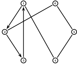
Figure 1: The communication graph.

Consider a network of six single-link manipulators with revolute joints actuated by a DC motor. The dynamics of the $i$-th manipulator is described by (14), with [28, 30]

$$x_{i} =\begin{bmatrix}x_{i1}\\ x_{i2}\\ x_{i3}\\ x_{i4}\end{bmatrix},\quad A=\begin{bmatrix}0&1&0&0\\ -48.6&-1.26&48.6&0\\ 0&0&0&10\\ 1.95&0&-1.95&0\end{bmatrix},\quad B=\begin{bmatrix}0\\ 21.6\\ 0\\ 0\end{bmatrix},$$

$$D_{1} =I,\quad D_{2}=\begin{bmatrix}0&1&0.4&0\end{bmatrix}^{T},\quad C=\begin{bmatrix}1&0&0&0\end{bmatrix},$$

$$f(x_{i}) =\begin{bmatrix}0&0&0&-0.333\mathrm{sin}(x_{i1})\end{bmatrix}^{T}.$$

Clearly, $f(x_{i})$ here satisfies (2) with a Lipschitz constant $\alpha=0.333$. The external disturbance here is $\omega=[w,-w,1.5w,3w,-0.6w,2w]^{T}$, where $w(t)$ is a one-period square wave starting at $t=0$ with width 2 and height 1.

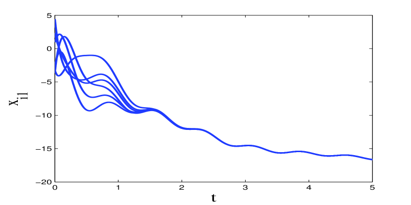
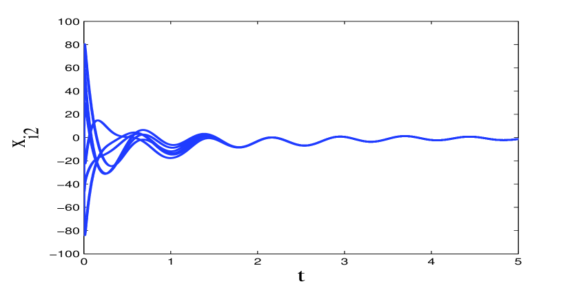
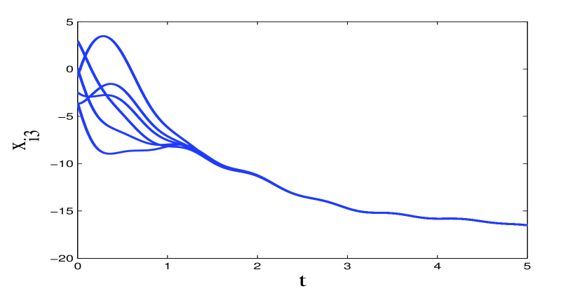
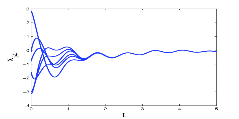
Figure 2: The six manipulators reach global consensus.

Choose the $H_{\infty}$ performance index $\gamma=2$. Solving the LMI (18) by using the LMI toolbox of Matlab gives a feasible solution:

$$P=\begin{bmatrix}0.4060&-0.9667&0.3547&-0.0842\\ -0.9667&67.6536&0.0162&-0.0024\\ 0.3547&0.0162&0.4941&-0.0496\\ -0.0842&-0.0024&-0.0496&0.0367\end{bmatrix},\quad\epsilon=29.6636.$$

Thus, by Algorithm 2, the feedback gain matrix of (3) is chosen as

$$K=\begin{bmatrix}-2.4920&-0.1957&1.4115&-3.8216\end{bmatrix}.$$

For illustration, let the communication graph $\mathcal{G}$ be given as in Fig. 1. It is easy to verify that $\mathcal{G}$ is balanced and strongly connected. The corresponding Laplacian matrix is

$$\mathcal{L}=\begin{bmatrix}2&0&-1&-1&0&0\\ -1&2&0&0&0&-1\\ 0&-1&1&0&0&0\\ -1&0&0&2&-1&0\\ 0&0&0&-1&2&-1\\ 0&-1&0&0&-1&2\end{bmatrix}.$$

The smallest nonzero eigenvalue of $\frac{\mathcal{L}+\mathcal{L}^{T}}{2}$ is equal to 0.8139. By Theorem 2 and Algorithm 2, the protocol (3) with $K$ chosen as above achieves global consensus with a $H_{\infty}$ performance $\gamma=2$, if the coupling strength $c\geq 36.4462$. For the case without disturbances, the state trajectories of the six manipulators under the protocol (3) with $K$ given as above and $c=37$ are depicted in Fig. 2, from which it can be observed that the global consensus is indeed achieved. With the zero-initial condition and external disturbances $\omega$, the trajectories of the performance variables $z_{i}$, $i=1,\cdots,6$, are shown in Fig. 3.

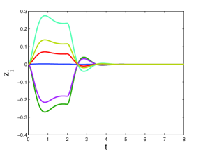
Figure 3: The performance variables $z_{i}$, $i=1,\cdots,6$.

7 Conclusion

This paper has considered the global consensus problems of a class of nonlinear multi-agent systems with Lipschitz nonlinearity and directed communication graphs. A two-step algorithm has been presented to construct a relative-state consensus protocol, under which a Lipschitz multi-agent system without disturbances can reach global consensus for a strongly connected directed communication graph. Another algorithm has been then given to design a protocol which can achieve global consensus with a guaranteed $H_{\infty}$ performance for a Lipschitz multi-agent system subject to external disturbances. An interesting topic for future research is to investigate the cooperative control problems of other types of nonlinear multi-agent systems.

References

• [1] R. Olfati-Saber, J. Fax, and R. Murray, “Consensus and cooperation in networked multi-agent systems,” Proceedings of the IEEE, vol. 95, no. 1, pp. 215–233, 2007.
• [2] W. Ren, R. Beard, and E. Atkins, “Information consensus in multivehicle cooperative control,” IEEE Control Systems Magazine, vol. 27, no. 2, pp. 71–82, 2007.
• [3] A. Jadbabaie, J. Lin, and A. Morse, “Coordination of groups of mobile autonomous agents using nearest neighbor rules,” IEEE Transactions on Automatic Control, vol. 48, no. 6, pp. 988–1001, 2003.
• [4] T. Vicsek, A. Czirók, E. Ben-Jacob, I. Cohen, and O. Shochet, “Novel type of phase transition in a system of self-driven particles,” Physical Review Letters, vol. 75, no. 6, pp. 1226–1229, 1995.
• [5] R. Olfati-Saber and R. Murray, “Consensus problems in networks of agents with switching topology and time-delays,” IEEE Transactions on Automatic Control, vol. 49, no. 9, pp. 1520–1533, 2004.
• [6] W. Ren and R. Beard, “Consensus seeking in multiagent systems under dynamically changing interaction topologies,” IEEE Transactions on Automatic Control, vol. 50, no. 5, pp. 655–661, 2005.
• [7] A. Rahmani, M. Ji, M. Mesbahi, and M. Egerstedt, “Controllability of multi-agent systems from a graph-theoretic perspective,” SIAM Journal on Control and Optimization, vol. 48, no. 1, pp. 162–186, 2009.
• [8] P. Lin and Y. Jia, “Distributed robust ${H}_{\infty}$ consensus control in directed networks of agents with time-delay,” Systems and Control Letters, vol. 57, no. 8, pp. 643–653, 2008.
• [9] Z. Li, Z. Duan, and G. Chen, “On $H_{\infty}$ and $H_{2}$ performance regions of multi-agent systems,” Automatica, vol. 47, no. 4, pp. 797–803, 2011.
• [10] Y. Cao and W. Ren, “Sampled-data discrete-time coordination algorithms for double-integrator dynamics under dynamic directed interaction,” International Journal of Control, vol. 83, no. 3, pp. 506–515, 2010.
• [11] Y. Gao, L. Wang, G. Xie, and B. Wu, “Consensus of multi-agent systems based on sampled-data control,” International Journal of Control, vol. 82, no. 12, pp. 2193–2205, 2009.
• [12] W. Ren, “On consensus algorithms for double-integrator dynamics,” IEEE Transactions on Automatic Control, vol. 53, no. 6, pp. 1503–1509, 2008.
• [13] P. Lin and Y. Jia, “Further results on decentralised coordination in networks of agents with second-order dynamics,” IET Control Theory and Applications, vol. 3, no. 7, pp. 957–970, 2009.
• [14] W. Ren, K. Moore, and Y. Chen, “High-order and model reference consensus algorithms in cooperative control of multivehicle systems,” ASME Journal of Dynamic Systems, Measurement, and Control, vol. 129, no. 5, pp. 678–688, 2007.
• [15] Z. Li, Z. Duan, G. Chen, and L. Huang, “Consensus of multiagent systems and synchronization of complex networks: A unified viewpoint,” IEEE Transactions on Circuits and Systems I: Regular Papers, vol. 57, no. 1, pp. 213–224, 2010.
• [16] Z. Li, Z. Duan, and G. Chen, “Dynamic consensus of linear multi-agent systems,” IET Control Theory and Applications, vol. 5, no. 1, pp. 19–28, 2011.
• [17] L. Scardovi and R. Sepulchre, “Synchronization in networks of identical linear systems,” Automatica, vol. 45, no. 11, pp. 2557–2562, 2009.
• [18] J. Seo, H. Shim, and J. Back, “Consensus of high-order linear systems using dynamic output feedback compensator: Low gain approach,” Automatica, vol. 45, no. 11, pp. 2659–2664, 2009.
• [19] M. Arcak, “Passivity as a design tool for group coordination,” IEEE Transactions on Automatic Control, vol. 52, no. 8, pp. 1380–1390, 2007.
• [20] A. Das and F. Lewis, “Distributed adaptive control for synchronization of unknown nonlinear networked systems,” Automatica, vol. 46, no. 12, pp. 2014–2021, 2010.
• [21] W. Yu, G. Chen, M. Cao, and J. Kurths, “Second-order consensus for multiagent systems with directed topologies and nonlinear dynamics,” IEEE Transactions on Systems, Man, and Cybernetics, Part B: Cybernetics, vol. 40, no. 3, pp. 881–891, 2010.
• [22] Q. Song, J. Cao, and W. Yu, “Second-order leader-following consensus of nonlinear multi-agent systems via pinning control,” Systems and Control Letters, vol. 59, no. 9, pp. 553–562, 2010.
• [23] Z. Li, Z. Duan, and G. Chen, “Global synchronised regions of linearly coupled lur’e systems,” Internatinal Journal of Control, vol. 84, no. 2, pp. 216–227, 2011.
• [24] Z. Qu, Cooperative Control of Dynamical Systems: Applications to Autonomous Vehicles. London, UK: Spinger-Verlag, 2009.
• [25] S. Boyd, L. El Ghaoui, E. Feron, and V. Balakrishnan, Linear Matrix Inequalities in System and Control Theory. Philadelphia, PA: SIAM, 1994.
• [26] T. Iwasaki and R. Skelton, “All controllers for the general $H_{\infty}$ control problem: LMI existence conditions and state space formulas,” Automatica, vol. 30, no. 8, pp. 1307–1317, 1994.
• [27] R. Rajamani, “Observers for Lipschitz nonlinear systems,” IEEE Transactions on Automatic Control, vol. 43, no. 3, pp. 397–401, 1998.
• [28] R. Rajamani and Y. Cho, “Existence and design of observers for nonlinear systems: relation to distance to unobservability,” International Journal of Control, vol. 69, no. 5, pp. 717–731, 1998.
• [29] R. Horn and C. Johnson, Matrix Analysis. New York, NY: Cambridge University Press, 1990.
• [30] F. Zhu and Z. Han, “A note on observers for Lipschitz nonlinear systems,” IEEE Transactions on Automatic Control, vol. 47, no. 10, pp. 1751–1754, 2002.