Resolving the terrestrial planet forming regions of HD113766 and HD172555 with MIDI
Abstract
We present new MIDI interferometric and VISIR spectroscopic observations of HD113766 and HD172555. Additionally we present VISIR 11m and 18m imaging observations of HD113766. These sources represent the youngest (16Myr and 12Myr old respectively) debris disc hosts with emission on 10AU scales. We find that the disc of HD113766 is partially resolved on baselines of 42–102m, with variations in resolution with baseline length consistent with a Gaussian model for the disc with FWHM of 1.2–1.6AU (9–12mas). This is consistent with the VISIR observations which place an upper limit of 014 (17AU) on the emission, with no evidence for extended emission at larger distances. For HD172555 the MIDI observations are consistent with complete resolution of the disc emission on all baselines of lengths 56–93m, putting the dust at a distance of 1AU (35mas). When combined with limits from TReCS imaging the dust at 10m is constrained to lie somewhere in the region 1–8AU. Observations at 18m reveal extended disc emission which could originate from the outer edge of a broad disc, the inner parts of which are also detected but not resolved at 10m, or from a spatially distinct component. These observations provide the most accurate direct measurements of the location of dust at 1–8AU that might originate from the collisions expected during terrestrial planet formation. These observations provide valuable constraints for models of the composition of discs at this epoch and provide a foundation for future studies to examine in more detail the morphology of debris discs.
keywords:
circumstellar matter – infrared: stars.1 Introduction
Since first being identified using data from the IRAS satellite, the debris disc phenomenon has been the subject of intense study. Spitzer surveys have confirmed that such discs, thought to be the debris material left over at the end of the planet formation process, are present around 15% of nearby stars (see e.g. Wyatt 2008 and references therein). The spectral energy distribution (SED) of the dust emission in most debris discs peaks at 60m, implying that the dust is cool (80K), and resides in Kuiper belt-like regions (10AU) in the systems. However, some systems have hot dust on scales 10AU. The current tally of known hot debris discs is 20 across spectral types A–M (13 catalogued in Wyatt et al. 2007a, b, and 7 recently discovered with AKARI; Fujiwara et al. 2009). This tally includes systems with multiple components where the hottest component lies at 10AU, such as Tel (Smith et al., 2009a) and Leo (Stock et al., 2010). For some multiple dust component systems (e.g. Corvi, Smith et al. 2009b and references therein) it is suggested that the hot dust component may be fed by a parent planetesimal belt coincident with the cooler dust belt. For systems without a known cold dust component, alternative models for the origin of the hot dust must be sought.
| Science targets | ||||||||
| Source | Spectral type | Age | RA | Dec | at 10m | at 10m | Stellar angular size | Predicted disc size |
| HD | Gyr | mJy | mJy | mas | mas | |||
| 113766 | F3V | 16a | 13 06 35.8 | -46 02 02.01 | 94 | 2359 | 0.0480.003 | 13, 31–69c |
| 172555 | A5V | 12b | 18 45 26.9 | -64 52 16.53 | 721 | 973 | 0.270.01 | 198d |
| Standard stars | ||||||||
| Source | Spectral type | RA | Dec | at 10m | Angular size | Instrument | ||
| HD | mJy | mas | ||||||
| 111915 | K3.5III | 12 53 06.91 | -48 56 35.93 | 13797 | VISIR | |||
| 110253 | K2III | 12 41 09.67 | -44 06 04.27 | 1065 | 0.870.02 | MIDI | ||
| 112213 | M0III | 12 55 19.43 | -42 54 56.50 | 14542 | 3.160.02 | MIDI | ||
| 116870 | K5III | 13 26 43.17 | -12 42 27.60 | 10416 | 2.580.01 | MIDI | ||
| 152186 | K1III | 16 55 34.43 | -60 40 38.77 | 785 | 1.000.02 | MIDI | ||
| 156277 | K2III | 17 21 59.48 | -67 46 14.30 | 7004 | 2.000.01 | VISIR, MIDI | ||
| 169767 | G9III | 18 28 49.86 | -49 04 14.10 | 9006 | 2.150.01 | MIDI | ||
| 171212 | K1III | 18 36 41.43 | -56 13 37.12 | 754 | 1.540.02 | MIDI | ||
| 171759 | K0III | 18 43 02.14 | -71 25 21.20 | 12640 | 2.680.01 | TReCS, MIDI | ||
a Age taken from Sco-Cen association membership. b Age from membership of Pic moving group. c From fit to IRS spectra by Lisse et al. (2008). d From fit to IRS spectra by Lisse et al. (2009). Estimated values of arise from fitting a Kurucz model photosphere of appropriate spectral type to the 2MASS K band measured photometry. For the science targets is determined from the Spitzer IRS spectra of the target after subtraction of the photospheric model. For the standard targets used in MIDI observations angular size was taken from the CalVin tool available at http://www.eso.org/intruments/midi/tools where available (HDs 112213, 116870, 156277, 169767, and 171759). For the remaining standard targets and the stellar components of the science targets the angular size was estimated by assuming that the stars have a diameter typical for their spectral type (taken from Cox 2000) and using the Hipparcos parallax to determine their distance. Standard stars are used as calibrators for the instruments listed (see text for details).
Amongst these sources, HD113766 (16Myr old) and HD172555 (12Myr old, Zuckerman 2001) are the youngest. They also have some of the brightest levels of excess (Wyatt et al. 2007a, b; see Table 1 for further source details). The favoured interpretation for the emission observed around these sources is that we are witnessing ongoing terrestrial planet formation (Kenyon & Bromley, 2004), since a detailed analysis of the Spitzer IRS spectra of both sources indicates that the dust composition is similar to that expected from the catastrophic disruption of terrestrial planet embryos (Lisse et al., 2008; Lisse et al., 2009). However, alternatives to the planet formation origin model for such hot emission do exist, including the scattering of comets from tens of AU in the system (Gomes et al., 2005), the sublimation of one supercomet (Beichman et al., 2005), a recent collision between two massive asteroids (Song et al., 2005), a disc of planetesimals on highly eccentric orbits (Wyatt et al., 2010), or that it is in fact a steady-state phenomenon. This has recently been suggested for the HD69830 system (Heng, 2011), which had previously been identified as a host of transient debris emission, (Wyatt et al., 2007a).
A correct interpretation of the hot dust depends critically on its radial location. We expect different dust distributions from the different theories for the origin of the dust, e.g., a population of comets scattering inwards would be expected to be observed at multiple distances from the star (the parent belt location and the dust sublimation radius) whereas dust from terrestrial planet formation would be expected to be confined to a narrow ring. Modelling the SED provides poor constraints on the radial distribution of the dust, as one may either: (i) underestimate the size of the dusty region, because the emitting grains are small and hotter than blackbody (observed discs can be a factor of 3 larger than predicted due to this effect, Schneider et al. 2006); or (ii) overestimate the size of the disc, because the dust is in an extended distribution (for example the predicted size of the Lep disc was more than double the observed size as multiple disc components over a range of distances from the star had been fit by a single disc temperature, see Moerchen et al. 2007; Smith & Wyatt 2010). The most direct way to resolve these ambiguities is with very high spatial resolution observations. In this paper we present VISIR imaging of HD113766 together with VISIR spectroscopy and MIDI observations of both HD113766 and HD172555. We also present a re-analysis of archival TReCS imaging of HD 172555. These observations are compared with models for the distribution of the dust and constraints placed on the location of the emitting material.
2 Observations with 8m instruments
2.1 VISIR imaging and photometry of HD113766
Standard
HD113766A
Residual
HD113766B
N band

Q band
High resolution imaging with 8m-class telescopes can reveal debris disc structure on 05 scales which corresponds to tens of AU for nearby stars (see e.g. Smith et al. 2009a). We used VISIR on the VLT to search for emission around HD113766 on such scales. Observations were performed in filters SiC (m, m, hereafter referred to as N band) and Q2 (m, m, hereafter referred to as Q band) under observing program 079.C-0259(A) in April 2007. Observations were performed in a perpendicular chop-nod pattern. The science observations were calibrated using observations of HD111915 taken from the Cohen catalogue of mid-infrared standards (Cohen et al., 1999). Standard star observations were performed immediately before and after the science observations to allow measurements of variations in photometry and the PSF, crucial in the search for extended emission. A summary of the observations is given in Table 2. Data reduction was performed with custom routines, the details of which are given in Smith et al. (2008). Data reduction involved determination of a gain map using the mean values of each frame to determine pixel responsivity (masking off pixels on which source emission could fall, equivalent to a sky flat). In addition a dc-offset was determined by calculating the mean pixel values in columns and rows (excluding pixels on which source emission was detected) and this was subtracted from the final image to ensure a flat background. Pixels showing high or low gain, or those that showed great variation throughout the observation, were masked off. Finally, the four images (two negative, two positive) resulting from the perpendicular chop-nod pattern were co-added to give a final image for HD113766 and observations of the standard. The center of each image was determined through fitting with a two-dimensional Gaussian, with the center of each image aligned in the co-addition step. Aperture photometry centered on the Gaussian peaks of the final images was performed using 1″radius apertures (noise levels were determined from an annulus with inner radius 2″and outer radius 4″). The calibrated flux found in the final images was 167342mJy for HD113766A at N and 189534mJy at Q. These uncertainties include calibration errors of 2% and 6% respectively determined from variation in calibration factors between the two standard star observations in each filter. These fluxes are compatible within the errors with the IRS photometry, which taken over the filters used here are 1599mJy at N and 1867mJy at Q.
| OB ID | Filter | Int. time (s) | Object type | Star |
|---|---|---|---|---|
| 265452 | Q2 | 400 | Cal | HD111915 |
| 265453 | Q2 | 1800 | Sci | HD113766 |
| 265450 | Q2 | 400 | Cal | HD111915 |
| 265455 | SiC | 105 | Cal | HD111915 |
| 265457 | SiC | 900 | Sci | HD113766 |
| 265456 | SiC | 105 | Cal | HD111915 |
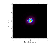
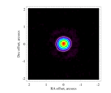
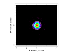
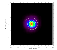
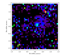
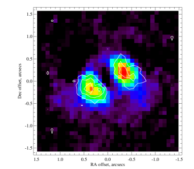
The final VISIR images of the PSF reference (standard star image) and HD113766 are shown in Figure 1 (first and second columns respectively; top row is N band images, Q band images are shown in the bottom row). The final images are shown with contours at 10, 25, 50 and 75% of the peak. There is no evidence that there is extended emission around HD113766 in either the N or Q band images from the contour lines (as compared to those of the standard star; low level ellipticity in the N band standard star image is below a 3 significance level). To search for low-level extended emission the standard star image was scaled to the peak of the HD113766 image (in each band) and subtracted from the science image. The result is shown in the third column of Figure 1 (labelled residual). The source appearing to the North-West in the N band is a known binary companion discussed in the following paragraph. Excluding this source the residual images are compatible with the noise levels of the image. These images reveal no evidence for residual emission extended beyond the PSF in either band.


HD113766 is a known binary star with F3/F5 components. In the Hipparcos catalogue the B component is listed at an offset of 1335 at a position angle of 281∘ East of North from the primary. A source is clearly seen in the residual image taken with filter SiC at an offset of 137 at a PA of 279∘ East of North from the primary, based on Gaussian fits to determine the centers of the source images. At a parallax distance of 131pc this translates to an on-sky separation of 157AU. Aperture photometry at this location gives a flux of 495mJy for the binary in the N band. We see no significant flux at this location in the Q band image. This is consistent with a SED fit to the binary companion (a Kurucz profile of spectral type F5 scaled to the Hipparcos V band flux of the binary companion) which predicts a flux of 14mJy. Such emission is below the 1 detection threshold on the Q band image (1 in a 1″radius aperture is 15mJy). The contours on the HD113766B image in the N band (Figure 1 top right) are more uneven than the PSF as measured on the standard star, but there is no evidence of extended emission from the contours. As a further test the PSF image scaled to the peak of the binary companion was subtracted from the HD113766B image and the residual emission was found to be consistent with the noise on the image.
As a final test for extended emission around HD113766 the surface brightness profiles of the standard star images and HD113766 were examined. There is no evidence in these profiles for extended emission around HD113766 beyond the shape seen for the point-like standard star targets (Figure 2). If we take sub-integrations of the science observations and the standard star observations to consider the variation in the profile we have 2 sub-integrations of the standard star observation and 5 for HD113766 at N. The mean and standard deviations for the FWHM measurements for these sub-integrations are 03240002 for the standard star and 03220004 for HD113766. For the Q band images we have 4 sub-integrations of the standard star observation and 11 for HD113766. The mean and standard deviations of the FWHM measurements for these sub-integrations are 0498 0006 for the standard star and 04980002 for HD113766. These results also show no evidence for extended emission around HD113766 in either band. The increase in FWHM in the Q band compared to the N band is exactly what would be expected from the increased diffraction limit at the longer wavelength of observation.


Standard
HD172555
Residual
N band

Q band
In addition to examination of the images, surface brightness profiles and FWHM measurements, we use the technique presented in Smith et al. (2008) to assess the limits of our detection capability for extended emission. For each photometric band we created a series of disc models comprising rings of radius with “widths” (so that the inner radius of the disc would be , outer radius ) and different inclinations to the line of sight. The rings were assumed to have constant surface brightness. These model images were added to point sources, representing the stars, and these sums then convolved with a PSF model. The final model images of the discs plus stars were then subjected to the testing detailed in Smith et al. (2008). In brief, this testing consisted of subtracting the point-like emission (by scaling the PSF model to the peak of the image in the same way as the residual images above were created), multiplying the residual image by a mask, and testing this final image for emission above the noise level of the image. The masks blank all pixels apart from a region of optimal size and shape to detect the disc emission based on the geometry of the disc (optimal regions were determined by extensive modelling of optimising disc detectability depending on source geometry presented in Smith et al. 2009b). This allowed us to determine what disc parameters (and levels of disc flux, which were also varied) would have led to a detection of extended emission. 111The science images were also tested in the same way, subtracting both HD113766A and HD113766B by subtracting scaled standard star images. The emission in the masked regions (using a full range of masks for a range of disc geometries) was always found to be consistent with the noise levels in the images. The resulting 3 extension limits on the location of the excess emission are shown in Figure 3. For a given radius the limiting flux required for a 3 detection of extended emission is shown for a disc centered on the star with median radius at that radius, with a full radial extent dependent on the geometry of the disc. The limits suggest that for narrow ring models in the N band, with a flux equal to the disc flux inferred from the IRS spectrum (1599mJy), any face-on or edge-on discs greater than approximately 013 (17AU) in radius would have been detected in our data. Similarly in the Q band, for discs with 1867mJy of flux (determined by subtracting the predicted photospheric emission from the Spitzer IRS spectrum of HD113766) any extended disc larger than 0135 (18AU) in radius would have been visible at the 3 level. The photospheric contribution was calculated from a scaled Kurucz model photosphere as outlined in Table 1. Detailed modelling by Lisse et al. (2008) suggests that the warm emission comes from a region 1.8AU (13mas)from the primary, and icy grains are situated in a belt at 4–9AU (31–69mas) from the star. Additional ice at 30–80AU (23–61mas) in the Lisse et al. model contributes to longer wavelength excess but has very low emission at the VISIR wavelengths. The limits from the VISIR imaging presented here are consistent with the fit of Lisse et al. (2008).
The imaging data of HD113766 would have detected extended disc structure at the levels detected in the IRS spectrum on scales of 17AU. The lack of evidence for any extended emission in either the N or Q band images therefore allows us to place an upper limit of 17AU on the extent of dust emission around the source.
| Filter | Int. time (s) | Object type | Star |
|---|---|---|---|
| Si5 | 60 | Cal | HD171759 |
| Qa | 60 | Cal | HD171759 |
| Qa | 640 | Sci | HD172555 |
| Si5 | 640 | Sci | HD172555 |
| Si5 | 60 | Cal | HD171759 |
| Qa | 60 | Cal | HD171759 |
2.2 TReCS imaging of HD172555


We do not have VISIR imaging of HD172555, but recently 8m-imaging data of this target has been presented by Moerchen et al. (2010). In 680s of on-source integration with TReCS in both the Si-5 (m, hereafter N band) and Qa (m, hereafter Q band) filters the authors found no evidence for extended emission. However, Pantin & di Folco (2011) recently presented Lucky Imaging of this target with VISIR which suggested that HD172555 appears extended in the Q band, although not in the N band. To explore this issue further, we have obtained the TReCS raw data presented in Moerchen et al. (2010) from the Gemini Science Archive. The data were reduced using the same custom procedures used for our VISIR imaging of HD113766. The science observations were calibrated using observations of the standard star HD171759, taken immediately before and after the science observations. A summary of the observations is given in Table 3. In contrast to the VISIR imaging, the TReCS observations were performed with a parallel chop-nod pattern. As the off-beams are unguided which can effect the shape of the PSF, we only use the guided images of the targets in our analysis. Sub-integrations on the targets were co-added using the Gaussian centering techinque employed for the VISIR observations of HD113766. Aperture photometry centered on the Gaussian peaks of the final images was performed using 1″radius apertures (noise levels were determined from an annulus with inner radius 2″and outer radius 4″). The calibrated flux found in the final images was 112067mJy for HD172555 at N and 103985mJy at Q (errors include calibration errors of 3% and 8% respectively determined from variation in calibration factors between the two standard star observations in each filter). These values are consistent with those quoted in Moerchen et al. (2010; values were listed as 1155116mJy at N and 1094164mJy at Q including fiducial 10% and 15% calibration uncertainties).
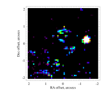
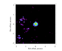
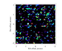
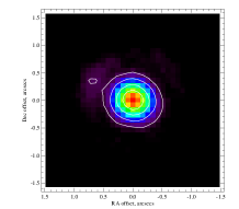
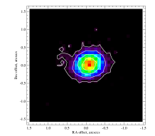
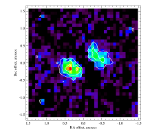
The final images for the PSF reference (standard star) and HD172555 are shown in Figure 4. The final images are shown with contours at 10, 25, 50 and 75% of the peak. There is no evidence for extension in the N band image of HD172555. In the Q band image we see some evidence of greater ellipticity in the image of HD172555 than is seen in the PSF reference image. This is confirmed in the residual image, which is created by subtracting from the science image the PSF reference image scaled to the peak of the science image. The residual image is shown in the right-hand column of Figure 4. We see two clear lobes of extended emission in the Q band residual image aligned along a position angle of 110∘EoN, but no significant emission in the N band residual image. The total flux subtracted from the Q band image of HD 172555 to obtain the residual image is 934 mJy, much higher than the predicted flux from the stellar photosphere in this filter of 202mJy.


To test whether the emission we observed is truly significant, or the result of a varying PSF, we examined the science and standard star image profiles in sub-integrations (single chop-nod cycles) on the targets. We have 6 sub-integrations on the standard star object and 32 on HD172555 in each band. Taking a strip centered over the peak of the image of 3 pixels’ width (009/pixel) and averaging across this width we create a 1-d profile of the image for each sub-integration. These profiles are taken at 110∘ EoN (to coincide with the residual emission peaks at Q) and 20∘ EoN (perpendicular to the residual peaks). The profiles are shown in Figure 5. We see that in the N band there is no evidence that the profiles of HD172555 are more extended than the profiles of the standard star target. In the Q band the image of HD172555 is extended in the 110∘EoN direction, but not at 20∘ EoN. This suggests that if the extended emission we are viewing arises from a disc, then we are viewing the disc close to edge-on, or it is a highly elliptical disc. The profiles in the Q band of the science target are quite noisy. As a final test of the extension detection, we examine the FWHMs of the sub-integration profiles. The FWHMs are determined by fitting a 1-dimensional Gaussian to each profile. The results are shown in Figure 6. It is clear from this plot that the FWHMs of the HD172555 images are always larger than the FWHM of the standard star images at 110∘EoN in the Q band. At 20∘ EoN and at both angles in the N band, the FWHMs of HD172555 are consistent with those measured for the standard star target.
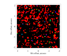
The disc models used in the extension limits testing for HD 113766 were then used to determine the approximate size of the extended emission. The models (of varying size, thickness, inclination and rotated to different position angles, see previous section 2.1 for a description) were added to point sources representing the star and any unresolved excess and convolved with the PSF (the standard star image). These model images were compared to the image of HD172555 by subtracting the model image from the science image (scaling to the peak) and comparing the residuals with the noise on the image. Using a calculation to determine the best fitting model we find that a disc of radius 027 (7.9AU at 29.2pc), width , inclined at 75∘ to the line of sight lying at a position angle of 120∘ EoN provides the best fit to the data. In this best-fitting model 65% of the total flux arises from the extended emission, suggesting a point-like flux of 363mJy, exceeding the 202mJy predicted to arise from the star. The best fitting model image is shown, after subtracting the scaled PSF image, in Figure 7 which can be directly compared to the residual image in Figure 4. The contours plotted on this figure are from the HD172555 residual image, and show that the model does indeed reproduce the main features of the extended emission. To determine limits on the radius of the disc model, we sum the values over all values of the other parameters tested (, inclination, position angle and flux in the disc). Using the percentage points of the distribution we find that discs with radii 009 031 (2.6–9.1AU) fit the observed emission within 3. Using the same technique for the other model parameters we obtain the following limits: ; inclination ; EoN position angle EoN; 14% percentage of total flux in disc 74%.
The focus of this paper is the size and geometry of the dust emitting at 10m. As we see no extension in the N-band image, we use the same procedures adopted in the VISIR imaging of HD113766 to place a limit on the size and geometry of the HD172555 disc in the N band. The results are shown in Figure 8. These limits suggest that the emission in the N band lies at 027 (7.9AU) and thus if the material dominating the N band emission was coincident with that dominating the Q band extended emission we would have expected to detect extension, making this result a significant non-detection. The size limit matches the size of the best fitting model to the extended emission detected in the Q band image. As this model showed some evidence for residual unextended emission, this may suggest that there are two populations of dust in this system. In this case the excess around HD172555 is a possible multiple component disc like that seen around other main sequence stars (e.g. Tel Smith et al. 2009a). However, it is also possible that we are observing a more extended disc, and that the N and Q band data are probing the inner and outer parts of the distribution due to their greater sensitivity to hotter and cooler dust in the disc respectively. This would also account for the apparent unresolved component in the Q band image, as there would still be some emission arising from inner part of the disc observable in the Q band.

2.3 VISIR spectroscopy
Detailed spectra of both our science targets have been obtained with IRS on the Spitzer Space Telescope (Chen et al., 2006). As discussed in Smith et al. (2009b) the measurements of photometry with MIDI suffer from poor background subtraction. It is helpful therefore to use the IRS spectra as reference total photometry for comparison to the correlated fluxes measured with MIDI. However, these spectra were obtained in a much broader slit than is used in MIDI observations (37 or 47 used in IRS; MIDI slit is 052 wide). It is thus possible that extended emission caught in the IRS slit would not be observed in the MIDI slit. The binary companion to HD113766 must also be ruled out as a source of excess emission.


To avoid any biasing of the interferometric visibilities which could arise from assuming a higher total flux than falls within the MIDI slit, we obtained VISIR spectroscopy of both science targets in low resolution mode (R350 at 10m) with a 075 slit (program ID 083.C-0775(E)). Two filters were used to examine the short and longer wavelength ranges covered by MIDI ( = 8.8m range 8–9.6m, hereafter filter 8.8; = 11.4m range 10.43–12.46m, hereafter filter 11.4). The observations were performed in chop-nod mode with standard star observations taken immediately before and after each science observation (Table 4 summarises the observations).
| Date | Target | Filter | Int. time (s) |
|---|---|---|---|
| 11th May 2009 | HD111915 | 8.8 | 240 |
| 11th May 2009 | HD113766 | 8.8 | 900 |
| 11th May 2009 | HD111915 | 8.8 | 240 |
| 11th May 2009 | HD111915 | 11.4 | 240 |
| 11th May 2009 | HD113766 | 11.4 | 600 |
| 11th May 2009 | HD111915 | 11.4 | 240 |
| 25th May 2009 | HD156277 | 8.8 | 240 |
| 25th May 2009 | HD172555 | 8.8 | 900 |
| 25th May 2009 | HD156277 | 8.8 | 240 |
| 7th July 2009 | HD156277 | 11.4 | 240 |
| 7th July 2009 | HD172555 | 11.4 | 600 |
| 7th July 2009 | HD156277 | 11.4 | 240 |
The observations were reduced with the VISIR pipeline procedures available at http://www.eso.org/sci/data-processing/software/pipelines/. Calibration was performed using an average of the two standard star observations obtained either side of the science observations. The standard stars fluxes were taken from Cohen et al. (1999) models for the mid-infrared standards used. We plot the observed spectra in Figure 9.
The VISIR spectroscopy of HD113766 was performed on one night, with the observation block (standard star HD111915, science target HD113766 and the standard star) in filter 11.4 taken immediately after the observation block in filter 8.8. The final observed spectrum looks very similar in shape to the IRS spectrum of HD113766, although it is lower everywhere by a factor of 1.3. This difference is not due to the binary component which fell within the slit of the IRS spectroscopy but outside the slit in the VISIR observations, because this source contributes only an average of 2% to the total flux across the 8–13m range (from scaled Kurucz model photosphere as described in Table 1 and the previous subsection). Geers et al. (2007) found that when using Spitzer IRAC photometry to calibrate VISIR N band spectra errors in absolute calibration could be as large as 30%, consistent with the difference between the VISIR and IRS spectra of HD113766 seen here. We also obtained archival IRS spectra of the standard star HD 111915. As the spectral ranges of VISIR and IRS are different, this allowed a comparison of the VISIR and IRS spectra of the standard star in the longer wavelength observation with VISIR only. A comparison of the IRS spectra reduced using pipeline routines shows that the calibration factor was varying over the course of the longer wavelength observation (we cannot test the stability of the calibration for the shorter wavelength observations as there is no overlap with the IRS spectra). The difference between the IRS and VISIR spectra was a factor of 1.07 and 1.15 for the VISIR calibration observations taken before and after the science observation, although again the shape of the spectra was consistent between the two. Although these differences are not as large as the factor of 1.3 observed for the science target, the difference between the two indicates that the absolute calibration was quite unstable during these observations. Within the errors of absolute calibration for VISIR, we see no evidence for extended emission detected in the IRS spectroscopy that would fall outside the MIDI slit. It is also worth noting that we do not see evidence for temporal evolution in the emission (within the calibration errors). The prospect of temporal evolution of the excess emission around HD 69830 (another star with bright levels of excess in the terrestrial planet region) has recently been ruled out (Beichman et al., 2011), but this remains a possibility for a star undergoing planet forming collisions. Photometry from the IRAS database (obtained in 1983; Beichman et al. 1988) gives a flux of 159080mJy at 12m. The Spitzer Space telescope IRS flux averaged over the finite bandwidth of the VISIR N band filter is 180392 mJy (data obtained in 2004; Chen et al. 2006). The VISIR photometry taken just 2 years prior to the VISIR spectroscopy presented in section 2.1 (167342mJy for HD113766A at N) is also consistent with a constant level of excess emission.
For HD172555 the difference between between the IRS spectrum of the target and that measured with VISIR is an average of 3% in filter 11.4, consistent with the variations observed between different standard star observations (measured to be 5%). The observations in filter 8.8 were taken on a different night, and the difference between the IRS spectrum and VISIR spectrum is found to be closer to 13%. Taken separately, the two sections of the VISIR spectrum again appear to be simply scaled versions of the IRS spectrum. The apparent sharp slightly offset peak in the VISIR spectrum at 9.5m is consistent with the flatter peak between 9.2–9.5m seen in the IRS spectrum within the uncertainty on the spectrum. The difference in calibration on different nights is the likely cause of the difference in scale factors for the observations in filters 8.8 and 11.4. In both cases the differences are within the 30% absolute calibration uncertainty found by Geers et al. (2007). There are no IRS observations of the standard star HD 156277 in the Spitzer archive.
Although the errors in absolute calibration for the VISIR spectroscopy are large, the shape of the spectra for HD113766 and HD172555 agree with the shape of the IRS spectra for both targets. We would expect cooler emission to be further from the star and thus more likely to be excluded from the VISIR spectroscopy. As we do not see a preferential loss of flux in the VISIR spectra as compared to the IRS spectra at long wavelengths, there is no evidence on the basis of the spectroscopy for extended emission that would fall outside the MIDI slit being detected in the IRS spectra. The absolute offsets between the VISIR and IRS spectra are consistent with an expected uncertainty of 30%, and there is no evidence for temporal evolution in the flux levels from near contemporaneous measurements. The IRS spectra of both targets shall therefore be used as a measure of the expected total photometry for comparison to the correlated fluxes measured with MIDI, however the implications if the VISIR spectrum had measured the true flux of the HD 113766 system are discussed briefly in sections 3.2 and 4.3.1.
3 The MIDI observations
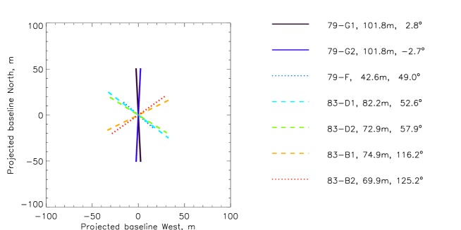
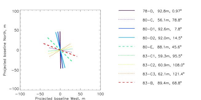
Observations were taken over several semesters through a combination of service and visitor mode observations. Table 5 lists the observing run IDs and dates of all observations, together with the baseline configurations used. All observations used MIDI on the UTs in the HIGH-SENS mode where the interferometric fringe exposures are followed by separate photometric exposures from each telescope in turn to measure the target spectrum through each beamline (for a summary see Smith et al. 2009b; further details can be found in the MIDI instruction manual or in Tristram 2007).
| Date | Observing | Baseline | Baseline | Baseline | Target | Target | Seeing | Flux | |
|---|---|---|---|---|---|---|---|---|---|
| ID | configurations | length (m) | Pos. Angle (∘) | name | type | ″ | ms | RMS | |
| 08/03/2007 | 078.D-0808(D) | UT1-UT3 | 102.2 | 36.52 | HD116870 | Cal | 1.76 | 2.0 | 0.0085 |
| 08/03/2007 | 078.D-0808(D) | UT1-UT3 | 92.8 | 0.97 | HD172555 | Sci | 0.70 | 6.2 | 0.0034 |
| 09/04/2007 | 079.C-0259(G) | UT1-UT3 | 101.8 | 2.8 | HD113766 | Sci | 0.72 | 3.1 | 0.0024 |
| 09/04/2007 | 079.C-0259(G) | UT1-UT3 | 102.2 | 9.0 | HD112213 | Cal | 0.83 | 2.6 | 0.0053 |
| 10/04/2007 | 079.C-0259(G) | UT1-UT3 | 101.8 | -2.7 | HD113766 | Sci | 0.59 | 3.0 | 0.0362 |
| 10/04/2007 | 079.C-0259(G) | UT1-UT3 | 102.3 | 3.0 | HD112213 | Cal | 0.74 | 2.8 | 0.0028 |
| 30/05/2007 | 079.C-0259(F) | UT1-UT2 | 48.7 | 41.7 | HD112213 | Cal | 1.52 | 1.0 | 0.0129 |
| 30/05/2007 | 079.C-0259(F) | UT1-UT2 | 42.6 | 49.0 | HD113766 | Sci | 1.73 | 0.7 | 0.0297 |
| 18/03/2008 | 080.C-0737(C) | UT3-UT4 | 57.9 | 85.8 | HD156277 | Cal | 0.81 | 5.7 | 0.0034 |
| 18/03/2008 | 080.C-0737(C) | UT3-UT4 | 56.1 | 78.8 | HD172555 | Sci | 0.59 | 7.6 | 0.0020 |
| 20/03/2008 | 080.C-0373(D) | UT1-UT3 | 88.9 | 20.4 | HD156277 | Cal | 0.88 | 6.4 | 0.0029 |
| 20/03/2008 | 080.C-0373(D) | UT1-UT3 | 92.6 | 7.8 | HD172555 | Sci | 0.61 | 9.7 | 0.0021 |
| 20/03/2008 | 080.C-0373(D) | UT1-UT3 | 100.7 | 12.8 | HD169767 | Cal | 0.51 | 9.0 | 0.0026 |
| 20/03/2008 | 080.C-0373(D) | UT1-UT3 | 92.0 | 14.5 | HD172555 | Sci | 0.49 | 10.3 | 0.0025 |
| 21/03/2008 | 080.C-0737(E) | UT2-UT4 | 89.3 | 60.8 | HD156277 | Cal | 0.82 | 4.6 | 0.0029 |
| 21/03/2008 | 080.C-0737(E) | UT2-UT4 | 88.1 | 45.6 | HD172555 | Sci | 0.71 | 4.8 | 0.0034 |
| 21/03/2008 | 080.C-0737(E) | UT2-UT4 | 89.4 | 70.7 | HD156277 | Cal | 0.79 | 5.8 | 0.0023 |
| 07/05/2009 | 083.C-0775(C) | UT3-UT4 | 58.7 | 90.0 | HD171759 | Cal | 1.29 | 1.8 | 0.0037 |
| 07/05/2009 | 083.C-0775(C) | UT3-UT4 | 59.3 | 95.5 | HD172555 | Sci | 1.10 | 1.8 | 0.0044 |
| 07/05/2009 | 083.C-0775(C) | UT3-UT4 | 60.8 | 103.9 | HD171212 | Cal | 1.10 | 1.7 | 0.0040 |
| 07/05/2009 | 083.C-0775(C) | UT3-UT4 | 60.2 | 102.7 | HD171759 | Cal | 1.14 | 2.0 | 0.0036 |
| 07/05/2009 | 083.C-0775(C) | UT3-UT4 | 60.9 | 108.0 | HD172555 | Sci | 0.95 | 2.0 | 0.0044 |
| 07/05/2009 | 083.C-0775(C) | UT3-UT4 | 62.4 | 135.4 | HD152186 | Cal | 0.82 | 2.0 | 0.0035 |
| 07/05/2009 | 083.C-0775(C) | UT3-UT4 | 61.2 | 114.7 | HD171759 | Cal | 0.98 | 2.3 | 0.0027 |
| 07/05/2009 | 083.C-0775(C) | UT3-UT4 | 62.1 | 121.4 | HD172555 | Sci | 1.49 | 1.5 | 0.0039 |
| 07/05/2009 | 083.C-0775(C) | UT3-UT4 | 62.4 | 128.2 | HD171212 | Cal | 1.14 | 1.9 | 0.0024 |
| 07/05/2009 | 083.C-0775(C) | UT3-UT4 | 62.0 | 130.2 | HD171759 | Cal | 0.76 | 2.9 | 0.0026 |
| 08/05/2009 | 083.C-0775(D) | UT1-UT3 | 86.2 | 49.6 | HD112213 | Cal | 0.47 | 6.2 | 0.0017 |
| 08/05/2009 | 083.C-0775(D) | UT1-UT3 | 82.2 | 52.6 | HD113766 | Sci | 0.46 | 6.7 | 0.0026 |
| 08/05/2009 | 083.C-0775(D) | UT1-UT3 | 75.8 | 55.7 | HD110253 | Cal | 0.52 | 6.8 | 0.0015 |
| 08/05/2009 | 083.C-0775(D) | UT1-UT3 | 75.7 | 55.2 | HD112213 | Cal | 0.51 | 5.8 | 0.0021 |
| 08/05/2009 | 083.C-0775(D) | UT1-UT3 | 72.9 | 57.9 | HD113766 | Sci | 0.49 | 6.2 | 0.0020 |
| 09/05/2009 | 083.C-0775(B) | UT2-UT4 | 74.6 | 113.0 | HD112213 | Cal | 0.97 | 3.0 | 0.0027 |
| 09/05/2009 | 083.C-0775(B) | UT2-UT4 | 74.9 | 116.2 | HD113766 | Sci | 1.16 | 2.6 | 0.0020 |
| 09/05/2009 | 083.C-0775(B) | UT2-UT4 | 67.6 | 126.0 | HD110253 | Cal | 0.71 | 4.9 | 0.0022 |
| 09/05/2009 | 083.C-0775(B) | UT2-UT4 | 69.9 | 125.2 | HD113766 | Sci | 0.76 | 4.9 | 0.0022 |
| 09/05/2009 | 083.C-0775(B) | UT2-UT4 | 62.6 | 132.9 | HD112213 | Cal | 0.71 | 4.8 | 0.0020 |
| 09/05/2009 | 083.C-0775(B) | UT2-UT4 | 89.4 | 65.9 | HD171759 | Cal | 0.56 | 5.9 | 0.0020 |
| 09/05/2009 | 083.C-0775(B) | UT2-UT4 | 89.4 | 68.8 | HD172555 | Sci | 0.62 | 5.6 | 0.0025 |
| 09/05/2009 | 083.C-0775(B) | UT2-UT4 | 89.4 | 74.6 | HD171212 | Cal | 0.80 | 4.5 | 0.0030 |
| 09/05/2009 | 083.C-0775(B) | UT2-UT4 | 89.2 | 78.0 | HD171759 | Cal | 0.56 | 5.6 | 0.0034 |
Seeing, (coherence time) and flux RMS are taken from
the ESO ambient conditions database
(http://archive.eso.org/cms/eso-data/ambient-conditions) for the
time at which the interferometric stage of the observations was
taken. Seeing is defined as the FWHM of a stellar image observed
with an infinitely large telescope at 500nm wavelength and at the zenith.
Flux RMS gives a measure of the background, with levels 0.05
indicating cloud cover and levels 0.02 indicating possible cloud
cover. Coherence times () of less than 3ms are considered very
fast, and indicate the presence of rapid atmospheric fluctuations that
are likely to have degraded the interferometric signal-to-noise.
Science observations were calibrated using the bright
standard star observations obtained before and after the science
observation where possible (i.e. when the science observation occured
between two standard star observations close both in time and
on-sky position). Otherwise only the observation of a bright
standard star (standard taken from the CalVin tool, see Table
1) closest in time to the science observation was used
for calibration purposes.


Reduction of the MIDI data was performed using the EWS software, available as part of the MIA+EWS package (see http://www.strw.leiden.nl/nevec/MIDI/index.html). Reduction followed the standard EWS routines. A summary of these steps is given below. Further details can be found in the manual available at the above link.
-
•
Frames were multiplied by a mask and compressed in the direction perpendicular to the spectral dispersion to obtain a one-dimensional fringe intensity spectrum. Following Smith et al. (2009b) we used masks determined from a fit to the total intensity (photometry) frames, as provided by the MIA reduction package, to best exclude source-free background pixels and thereby reduce noise levels.
-
•
The interferometric fringe data were aligned in time using an analysis of the measured group delay to remove components of the delay arising from instrumental and atmospheric effects. For further details of this procedure the reader should consult the EWS manual or Tristram (2007). Fringes were then averaged in time to produce a correlated flux (or more correctly correlated intensity as no flux calibration had been determined at this point). The correlated flux was then compared to the total source flux to give the source visibility .
In principle, the total source flux () could have been determined from the photometry frames observed following the fringe exposures with MIDI. The MIDI photometric data are consistent with the IRS spectra, however the variation between individual observations of the science target photometry with MIDI was as high as 30–40% across the full wavelength range. We have found that photometric measurements of faint targets with MIDI can often be rather noisy (see Smith et al. 2009b) and so instead we used the IRS spectra — which are not significantly different from the VISIR measurements (see Section 2) — to provide these data.
3.1 Visibility calibration
Two types of standard stars were used to calibrate the observations of the science targets. Bright standards were selected with the ESO CalVin tool (see http://www.eso.org/instruments/midi/tools). Much fainter standards were identified by searching for sources in the IRAS catalogue, within 25∘ of the science targets, that had similar 12m fluxes and that showed no evidence of binarity or variability. Our decision to utilise both faint and bright calibrators was motivated by a finding from our earlier studies of HD69830 and Corvi (Smith et al., 2009b) which showed tentative evidence of a loss of correlated flux at shorter wavelengths for faint targets. Our goal was to observe faint standards as though they were faint science targets to check for any bias in their measured visibilities. For these tests, we ensured that the 12m fluxes of the faint standards were consistent with the emission predicted from scaled Cohen et al. (1999) photospheres, and were confident that they showed no evidence of any excess emission (see next paragraph).
For those targets in the Cohen et al. (1999) catalogue of mid-infrared standard stars (HDs 111915, 116870, 156277, 112213) we used the Cohen spectrum of the target as the target flux. For the remaining targets we used Cohen templates for stars of the same spectral type scaled to the 10m flux listed in the CalVin tool (for HDs 169767 and 171759) or for the faint standard stars (HDs 171212, 152186 and 110253) scaled to the source’s listed 2MASS K band flux. The diameters for the bright standard stars used for the MIDI observations were taken directly from the CalVin tool. For the faint standards source diameters were determined by assuming that the stars had a diameter typical for their spectral type (taken from Cox 2000) and using the Hipparcos listed parallax to determine their distances. Our inferred source diameters for the standards are listed in Table 1.
The calibration of the target correlated flux was determined using the following equation:
| (1) |
where and were the correlated intensities measured in the fringe exposures of the ‘target’ and ‘calibrator’ respectively and was the visibility of the calibrator, assumed to be that of a uniform disc with the diameter given in Table 1. For we used the total flux of the calibrator taken from the Cohen spectrum of the standard (or the scaled Cohen spectrum, see paragraph above). The visibility of the target was then evaluated as
| (2) |
where was the total flux of the target, which in the case of the science targets was taken from the Spitzer IRS spectrum of the source.
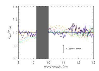
To determine the accuracy of our derived visibilities, we first examined the visibilities of the bright standard star targets when calibrated by other bright standard stars. By using pairs of standard star observations taken as close as possible in time, we were able to generate 10 independent visibility functions. These pairs of standard star observations were in general taken either side of science observations, and so were separated in time by roughly twice the time between a science and standard star observation. When corrected for the sizes of the standard stars used, these produced the visibility transfer functions shown in Figure 10. Note that the bandpass between 9.2–10m is subject to high levels of uncertainty due to ozone absorption, and so this region has been ignored in our analysis. The variation in transfer function level in the left hand panel of Figure 10 is indicative of the range of seeing mismatch between the observations of source and calibrator, with the values nearest to unity being associated with the use of calibrator stars closest in time and space. The weighted mean of the transfer functions across the whole spectral range gave a mean value of observed visibility/predicted visibility of 1.0020.057 (or 6%). To calculate the weighted mean we used weights derived from the errors on the correlated flux. These errors came from the variance found in the EWS reduction by splitting the fringe observations into 5 sub-integrations. We then calculated the weighted mean over the MIDI spectral range (excluding the 9.2–10m region which suffers from ozone absorption), and took a mean over all 10 pairs of standard stars to get the figure above.
In order to remove this source of variation, we scaled each transfer function so that its weighted mean in the range 8–9m was unity. These normalised transfer functions are presented in the right-hand panel of Figure 10. Most of the normalised transfer functions are very similar, but two of them deserve mention. The first, identified by a dashed line, is from an observation of HD112213 taken on 09/04/2007 (under observing ID 079.C-0259(G)) calibrated by an observation of the same target taken under the same observing configuration the next night. The second was derived from an observation of HD112213 taken on 09/05/2009 (under proposal 083.C-0775(B)) but has been calibrated using a “standard” located over 90∘ away on the sky (HD171759). These aberrant transfer functions highlight the need for very careful calibration strategies. Overall, we found the ratio of the transfer function in the range 10.5–11.5m (12–13m) to that at 8–9m for the remaining bright-bright pairings to be 1.0100.013 (1.0160.018). These data confirm that for our data the visibility functions for bright targets are likely to be calibrated to within 6%, and also that the differential visibility (the visibility with reference to that at a fixed wavelength) is a factor of 2–3 times more accurate than the absolute value of the visibility.
A similar analysis for our faint unresolved targets calibrated by bright standard stars is shown in Figure 11. The behaviour of these transfer functions is broadly similar, but there is definite evidence of curvature of the functions at the extremes of the MIDI bandpass. This is limited to the very first few spectral bins at the short wavelength end, but is more noticeable beyond a wavelength of 12m, where the data are increasingly noisy. We found that the weighted mean absolute values of the transfer functions across the MIDI wavelength range (excluding the 9.2–10m region) was 1.0350.072, and that the mean normalised transfer function between 10.5–11.5m relative to that at 8–9m was 0.9840.030. The equivalent value for the 12–13m bandpass was 1.0640.047. These data suggest that the visibilities of our faint targets can be measured to better than 10% (i.e. at a level consistent with what has been presented before, see e.g. Chesneau 2007), and that the differential visibility across the whole wavelength range is stable to better than 5%. Somewhat better accuracy can be expected if data at wavelengths 12m is excluded, typically by a factor of two.
3.2 MIDI observations of HD113766
The observations of HD113766 were calibrated using two bright standard star observations where possible (see Table 5). In these instances the average of the calibrated correlated flux using two standard star observations was used. The standard deviation between the two calibrations was added in quadrature to the error on the correlated flux as estimated from the time variation in the correlated intensity. This was derived by splitting the fringe integration into 5 sub-integrations and determining the standard deviation between the different sub-integration datasets.
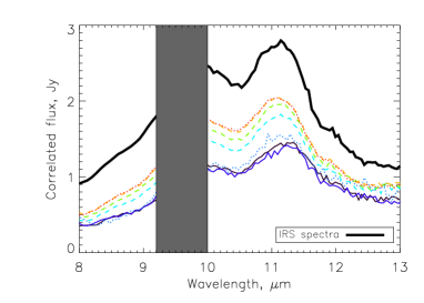
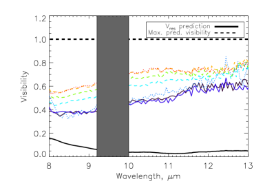
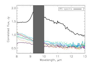
The correlated flux measurements for our 7 observations of HD113766 taken on various baselines (see Table 5) are shown in Figure 12, where the solid line is the IRS spectrum of the target. It is immediately clear that there is a significant difference between the correlated flux and the IRS spectrum. There also appears to be some difference between the observations taken under proposal 079.C-0259 and proposal 083.C-0775. This is further explored through comparison of their visibility functions.
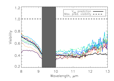
The visibilities calculated from the correlated flux measurement are shown in Figure 12. Interestingly, the visibility on baseline 79-F is somewhat lower than that measured on the longer but approximately parallel baseline 83-D (see caption to Figure 12 for description of labels and Table 5). This might indicate that rather than having a distribution like a Gaussian, the source emission is more complex. A ring for example would have an oscillating visibility function which would be higher on some longer baselines (see, e.g., Figure 5 of Dullemond & Monnier 2010 for an example of this). However, the observations on 79-F were taken under the poorest observing conditions in the study — the “flux RMS” and coherence time diagnostic metrics were particularly high — and under these conditions it is likely that the measured visibility was biased to a lower value. As a result, we did not use this visibility measurement as a constraint in the modelling of the HD113766 data presented in Section 4.
In the plot of the visibility function (Figure 12 top right) we have shown the behaviour for two extremal classes of targets, i.e. those that are completely unresolved and then those whose dust emission is fully resolved. For the first of these cases, we expect that the correlated flux is always equal to the total flux, and hence that the visibility is equal to unity at all wavelengths. In the second case, the situation is slightly more complicated, since both the potentially unresolved stellar contribution and the resolved dust emission need to be considered. For such targets, the visibility of the source will be given by
| (3) |
where and are the visibility of the disc and the star respectively, and are the fluxes of the disc and star respectively, and is the total flux (i.e. ). The stellar emission component in HD113766 is likely to be completely unresolved. It is a F3V-type star at a Hipparcos distance of 131pc, and so with an expected radius of 1.38 would subtend an angle of roughly mas, well beyond the resolving power of VLTI/MIDI. The minimum expected visibility, given that the star is expected to be completely unresolved (), is therefore the visibility in the event that the disc flux is completely resolved, , . We have labelled this visibility in Figure 12. As it is clear that for all baselines observed the visibility function lies between this and the maximum visibility of 1, the disc appears partially resolved on all baselines.
The visibility functions measured on similar baselines are consistent within the error levels expected for the visibility of a faint target (10%, see Section 3.1), The visibility functions measured on 79-G1 and 79-G2 are very similar to one another, as are the visibility functions measured on 83-B1 and 83-B2. It is also clear that the visibility functions measured on longer baselines are lower than those measured on shorter baselines (with the exception of 79-F as discussed above, and which we treat as unreliable). Solid lines are used in Figure 12 to denote the longest baselines, dotted lines the shortest and dashed lines intermediate baseline lengths.
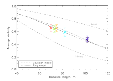
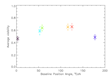
To display more clearly how the visibilities are varying with baseline length and position angle we show the average (weighted mean over the MIDI spectral range excluding the ozone dominated 9.2–10m region) visibility of HD113766 plotted against baseline length and position angle in Figure 13. Although the visibility is seen to change with wavelength (Figure 12 top right), to first order this effect can be attributed to the decreasing resolution of MIDI with increasing wavelength, and so we are unlikely to be biasing the data through this averaging. Excluding baseline 79-F, there is a drop in visibility with increasing baseline length, consistent with a simple source geometry such as a Gaussian. 222If we had instead used the VISIR spectrum as a model for the total flux of the HD 113766 system, then the calculated visibilities would be higher, but still exhibit the same behavior, i.e. decreasing with baseline length. In this case the points would lie close to the 7mas model shown in Figure 13. Also shown in this figure are the visibilities plotted as a function of baseline position angle. Although the visibilities closest to 0 or 180∘ appear lower, these are the longest observed baselines. If we consider only baselines of similar lengths (83-D1, 83-D2, 83-B1 and 83-B2) there is no evidence for a change in visibility with baseline position angle that would indicate a non-circularly symmetric source distribution. More details on the limits we can place on the source geometry with these observations are discussed in Section 4.
3.3 MIDI observations of HD172555
Our observations of HD172555 have been taken over several semesters. Where possible, two bright standard star observations were used to calibrate the correlated flux measurements of this target (see Table 5). Errors were calculated in the same way as described for HD113766 in the previous subsection.
The calibrated correlated flux measurements from our 9 observations of HD172555 with MIDI (see Table 5) are shown in Figure 14. As for HD113766, the IRS spectrum has been over-plotted for comparison. These plots show rather similar correlated flux levels for all baselines. The degree of resolution of the target is better seen in the visibility functions of the target, also shown in Figure 14 in the right hand panel. As for HD113766, we have over-plotted the predicted visibilities for targets with fully unresolved ( across all wavelengths) and fully resolved () disks for reference.
These plots show that for observations 78-D and 83-C3 the observed visibilities are more than 10% lower than the predicted visibility in the case that the disc is fully resolved (). Although values lower than can be observed on intermediate baselines (when due to the phase jumps in its pattern, see Figure 5 of Dullemond & Monnier 2010 for an example of this behavior), the visibilities observed on similar baselines (e.g. 81-D1 and 83-C2 respectively) do not fall significantly below . We believe that the results on baselines 78-D and 83-C3 can be explained by a combination of calibration errors. The coherence times for the observations on baseline 83-C were very short, particularly for the third observation of HD172555 which has a significantly shorter coherence time than the observations of standard stars used to calibrate the observation (see Table 5). This could be the cause of the low visibility as we believe was the case for our observation on baseline 79-F for HD113766. Secondly, the observation on baseline 78-D was taken at the end of a night towards twilight and had to be calibrated by observations of a standard star offset from HD172555 by 95∘. As demonstrated in Section 3.1 large offsets between a science target and standard star are an obvious source of miscalibration, which we believe has occurred here.
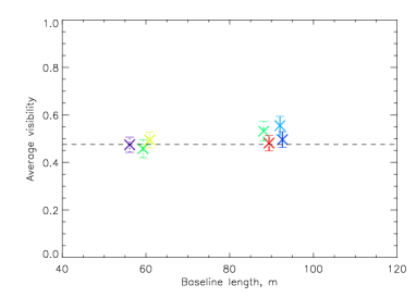
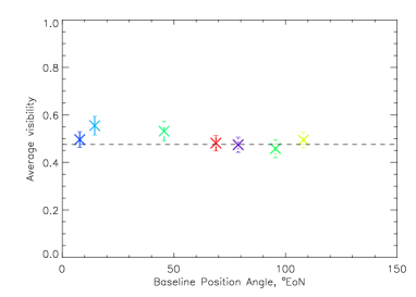
We can see that for all our baselines the observed visibility function for HD172555 is consistent with a completely resolved disc. High visibilities at 11.5m are likely due to the bias seen in observations of faint targets and can be compared with those seen for the faint calibrators (Figure 11 right). There is no evidence of a systematic decrease in visibility with increasing baseline length, suggesting that the excess emission is already completely resolved on the shortest baselines. There is tentative evidence that the mean observed visibility changes slightly with baseline position angle, which can be seen more clearly in Figure 15. Such a change with baseline position angle could reveal evidence of a clumpy structure, as may be expected as the result of a recent massive collision in the disc, the model favoured by Lisse et al. (2009). However, as the visibility seems to be smoothly changing with position angle (increasing with increasing position angle from 0–14∘ on baselines of similar length 80-D1 and 80-D2, and decreasing with increasing position angle from 46∘ on baselines of similar length 80-E and 83-B) this suggests a smoother, perhaps, elliptical structure for the emission. An ellipse with major axis oriented at 120∘ would have its lowest visibility on baselines at 120∘ EoN and its highest visibility on baselines at 30∘ EoN. Such an emission morphology could arise from an inclined circular disc or a truly elliptical disc. As we have complete resolution of the disc on the shortest baselines (56m, 80-C) we would expect such a disc to have a minimum radial size of at least 40mas (based on the resolving power of 56m aperture telescope at 10.5m). More detailed modelling of the observed visibility functions is presented in the following section.
4 Modelling the visibility functions
4.1 Visibility calculation
We consider several source geometries to try to fit the observed visibility functions around HD113766 and HD172555. The van-Cittert Vernicke theorem states that the normalised visibility function of a source is the normalised Fourier transform of the brightness distribution of the source. The simplest source geometry we consider is a circularly symmetric Gaussian. The source geometry is given by
| (4) |
where and are angular on-sky coordinates (in radians), is the full-width at half-maximum (FWHM) and . The visibility function of this source is then
| (5) |
where and are coordinates describing the spatial frequency of the brightness distribution such that , where and are the projections of the baseline vector on the two axes and is the wavelength of the observation (Berger & Segransan, 2007). For an elliptical Gaussian we parameterise the ellipticity by where (and ).
The Gaussian model provides a good model to an envelope, and offers a simple approximation to the overall source size. However, debris disc emission is expected to be ring-like in distribution. For a thin ring the source geometry is given by
| (6) |
(where is the Dirac delta function), then the visibility of such an object is given by
| (7) |
where is the 0th-order Bessel function and . For our debris disc models we follow the example of Malbet et al. (2005) and use a sum of thin rings to model the distribution and visibility function of a ring of finite thickness. The emission is distributed as the integration of all ring contributions given by equation 6 from to , and the visibility function of this finite thickness ring is similarly the integral of the corresponding Fourier transforms (visibility functions). For a disc inclined to the line of sight at an angle and at a position angle we simply consider the case where which represents the projected baseline in a new reference frame corresponding to a rotation of the array frame by the position angle with a compression factor of . To include the temperature distribution of the disc, we make the simplifying assumption that the disc is optically thin and the dust behaves like a blackbody, and so the temperature of each ring is dependent only on the distance from the star (as the stellar luminosity is fixed). Then
| (8) |
and the flux we can expect from our disc model is the integration of all the rings modified by the distance of the source from the observer, ,
| (9) |
We assume the disc surface density is flat and therefore is a constant. The visibility function corresponding to this model is therefore simply the normalised integration of the visibility function for the thin rings weighted by their flux.
These models are simple descriptions for the visibility function of the excess emission, . In our comparison to the data the final visibility model includes the contribution from the star which is completely unresolved by the interferometer (, see Section 3.2). The final value of is calculated according to equation 3.
Lisse et al. (2009) suggested that a possible origin for the emission around HD172555 is a recent massive collision between two large planetesimals/proto-planets. In this scenario we might expect the emission to arise from a clump offset from the central star. As the clump is offset from the central star, we cannot simply add the visibility functions scaled by their relative flux levels. For a multi-component function components at positions , in the plane of the sky with visibilities , the normalised visibility of the full function is
| (10) |
where is the flux of the component and is the total number of components. For a two-component model, the normalised squared visibility reduces to
| (11) |
which reduces to the familiar in the case that and .
4.2 Error calculation
To determine the goodness of fit of the models, and thereby calculate the best fitting model parameters, the calculation of the error terms on the visibility must be carefully considered. From equation 1, the error on the correlated flux arises from the terms , and . Here we have assumed that the error on the visibility of the calibrator is negligible. Errors on the calibrator diameters can be up to 5% (Verhoelst, 2005), and so at its highest the error on (from observation of HD112213 on baseline 79-G) is 0.5%, much lower than the other sources of uncertainty. The uncertainty on the calibrator flux is assumed to be 2% (, see Cohen et al. 1999).
The error on is determined by splitting the fringe observation of the target into 5 sub-integrations and determining the standard deviation from the mean value at each wavelength. The error on is the error from calibration. Here we use the visibility transfer functions (Section 3.1) to determine the error. At each wavelength value sampled in the MIDI range, we determine the mean and standard deviation of the visibility transfer functions for the faint standard stars. We check that the mean value is compatible with a value of 1 within the error given by the standard deviation, and adopt this standard deviation as our error on . The average value of this error across the MIDI range (excluding the ozone dominated 9.2-10m region) is 0.057. The error on the correlated flux is then given by
| (12) | |||||
To calculate the error on the visibility we can see from equation 2 that we need to add the error on the total flux, . As we have adopted the IRS spectra for our science targets, this is the error on the IRS spectra which itself is composed of the statistical uncertainty and calibration uncertainty on these observations. As the spectral sampling is different between IRS and MIDI, we use linear interpolation to determine the errors at the central wavelengths of the spectral bins of the MIDI data. Then the final error on the visibility is given by
| (13) |
with typical values of 6% (7%) for and 4% (3%) for for HD113766 (HD172555).
For the model visibilities equation 3 holds. We assume that the star has a fixed visibility of 1 () and has no error. We also assume that is perfectly known for any particular model. The error on is discussed in the above paragraph. The errors on and are more complex. They arise in part from the uncertainty on the total flux, and also from uncertainty in the relative contributions of the star and disc to the total flux. As a change in the value of would result in a systematic change in and , similarly a change in with no corresponding change in would result in a reciprocal change in . We therefore model the error on the term in a Monte Carlo manner. The scaling of the Kurucz model profile used to model the photosphere is determined by a minimisation over a range of scalings to find a best fit to the B and V band magnitudes of the stars as listed in the Hipparcos catalogue and the J H and K band magnitudes from the 2MASS catalogue. The percentage points of the distribution are used to determine a 1 limit on this scaling. The scaling used in the Monte Carlo modelling is taken from a Normal distribution with mean given by the best fitting scaling and standard deviation given by the level of the 1 error. The value of is also varied between the 1 error limits on the IRS spectrum (or rather the interpolated spectrum, see above). The value of is taken to be . The error term on is then taken from the standard deviation of 1000 random samplings, and is found to be typically at the 4% level for HD113766 and 6% for HD172555 averaged over the whole wavelength range. The final error on the model visibility is then
| (14) |
To test how well each model reproduces the observed visibilities we use the goodness-of-fit test. Typically this takes the form where is the number of data points, is some observed data with associated error and is a model with no error. As both our observational data and model have associated errors we use the ratio of the observed to model visibility and compare this to 1 (as if the model is a good fit to the data then ). The errors for both and must be included in . Our calculation then becomes
| (15) |
Here is the number of observations we have for a source and is the number of spectral channels. To calculate a reduced we divide the above by the number of data points (observations spectral channels) minus the number of free parameters in the model (1, the FWHM, for a circularly symmetric Gaussian; 4, the radius, thickness, inclination and position angle, for a ring). If we consider equations 2 and 3 we can see that in dividing by we cancel the term in . The errors from the IRS spectroscopy do not therefore appear explicitly in the calculation of . These errors do appear implicitly in the Monte Carlo calculation of the error on through the calibration and statistical errors. The final value of is given by the addition in quadrature of all the remaining error terms. As there is evidence of a bias in the visibility of low flux sources at wavelengths 12m (see Figure 11 and section 3.1) we exclude the 12m data from the model fitting.
4.3 Best fitting models for HD113766
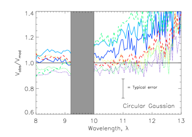
The observed visibility functions from the MIDI observations of HD113766 are consistent with a partial resolution of the excess emission. As a first attempt to model the distribution of the excess emission we tested circularly symmetric Gaussian models with a range of FWHM . We tested mas in 60 logarithmically-spaced steps. The visibility of the model was calculated according to the method described in Section 4.1, with the errors on the comparison of the model to the data and the goodness of fit of the model calculated as described in Section 4.2. The best fitting model is that with =10mas, which taken over the 8–12m range and the 6 baselines considered (excluding 79-F, see Section 3.2) has a reduced of 0.32.
Adopting an elliptical Gaussian model gives an additional two parameters to fit. As well as the FWHM , we also consider the ellipticity of the Gaussian , where , and the rotation of the model which represents the angle of the major axis of the elliptical Gaussian in degrees East of North. The ranges tested for each of these parameters were mas in 21 logarithmically-spaced steps, in steps of , and in steps of . The best fitting model ellipticity is , so a circular Gaussian model (with FWHM mas) provides the best fit.
Finally, we tested ring-like distributions for the excess. The parameters for these models were the radius of the center of the ring and the width of the ring . As the Gaussian modelling showed no evidence for inclined structure, we do not include inclination and position angle in our parameters for ring models. The parameter ranges tested were mas and (where describes a ring from 0–2). The best fitting model parameters are mas (so ring diameter is 12mas, similar to the best fitting Gaussian FWHM) and . The reduced for this model is 0.31.
4.3.1 Preferred model for HD113766
Despite the increased complexity, the ring models do not offer a much better fit to the data than the Gaussian models. A simple circularly symmetric Gaussian model with a FWHM mas offers a good fit to the data. This is in keeping with the initial first order approximation to the size of the emitting region shown in Figure 13. We see no evidence for a change in visibility with position angle (once the difference in baseline length is taken into account), and so a circularly symmetric distribution is to be expected to offer a good fit to the data. Using the percentage points of the distribution the 3 limits suggest a good fit can be achieved with mas (see Figure 16). The visibility of the best fitting Gaussian model, and the visibilities of models at the 5 limits (mas and 14mas), are plotted on Figure 13 (left). We also show for comparison the visibility of the best fitting ring model. 333If we had instead used the VISIR spectrum as our total flux in the analysis of the MIDI data, the visibility functions would be higher (see footnote 2. The resulting best fitting Gaussian model would have mas.

It is worth noting that for the best fitting models we achieve a reduced of . This would normally be termed an over-fit, and could be taken as evidence that the errors assigned to the data are too large. In this case the sources of error have been carefully considered in turn (see section 4.2). A more likely possibility is that the number of degrees of freedom is too high. We have used the number of wavelength bins multiplied by the number of observations as the number of data-points, and subtracted the number of free parameters for each model considered to determine the degrees of freedom. This calculation involves the implicit assumption that the data-points are independent, which for neighbouring wavelength bins for a particular observation will not be the case. This would mean that the values of reduced are underestimated. Calculation of degrees-of-freedom in such cases is complex (see Andrae et al. 2010 for a recent discussion). A better idea of the true absolute goodness-of-fit might be achieved by examination of for the best fitting model. This function is shown in Figure 17. For all baselines (excluding 79-F) the circular Gaussian with FWHM = 10mas provides a good fit to the observed visibility function.
4.4 Best fit models for HD172555
The observed visibility functions from MIDI observations of HD172555 suggest a completely resolved disc on all baselines. We first attempt to model the distribution of the excess emission using circularly symmetric Gaussian models with a range of FWHM . We tested mas (the predicted radius of the dust is larger for this target than for HD113766, see Table 1) in 60 logarithmically-spaced steps. The visibility of the model was calculated using the method described in Section 4.1, with the errors on the comparison of the model to the data and the goodness of fit of the model calculated as described in Section 4.2. The best fitting model is that with mas, which taken over the 8–12m wavelength range (excluding the ozone absorption region) and 7 baselines (excluding problematic observations 78-D and 83-C3, see Section 3.3) has a reduced of 1.0.
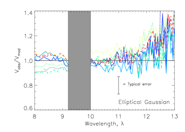
Testing elliptical Gaussian models suggests that an elliptical model provides a better fit. The best fitting parameters are found to be mas, and EoN. Such a configuration gives a slightly higher disc visibility along baselines at position angles close to 30∘EoN, and slightly lower visibility at baselines close to 120∘EoN. This orientation can be compared with Figure 15, which shows that observations at baselines similar to 30∘ have a slightly higher visibility. Confidence limits on these best fitting parameters are discussed further in subsection 4.4.1. The reduced for this best fitting model is 0.36.
We also tested ring-like distributions for the excess. The parameters for these models were the radius of the center of the ring , the width of the ring , the inclination of the ring to the line of sight and the position angle of the major axis . The parameter ranges tested were mas, , and EoN. The best fitting model parameters are mas, , and EoN. The reduced for this model is 0.38. This visibility model produces higher on baselines close to 30∘EoN and low () on baselines close to 120∘EoN (compare with Figure 15).
The model of Lisse et al. (2009) suggests that the emission from HD172555 might be the result of a recent massive collision in the system. If so, the emitting material might be expected to be concentrated in a clump rather than spread in a ring-like distribution. Dust emitting from a circumplanetary region would also look like a clump orbiting the star. A point-like clump at an offset from the point-like star would have a visibility of 1 on baselines along a position angle 90∘ from the direction of the offset of the clump from the star (e.g. if a point-like clump lay directly north of the star, then observations on baselines lying East-West, or at PAs of 90∘EoN, would have visibilities of 1). In the observed data all visibilities are 1. Along baselines in the direction of a point-like offset clump the visibility would be seen to oscillate in a sinusoidal manner, with maxima of 1, minima of (averaged over the MIDI wavelength range when , see equation 11), and period dependent on the distance between the clump and the central star. As all visibilities are compatible with a resolved disc at the 2 level (or better), and no visibilities are compatible with an unresolved source (at the level averaging over the 8–12m MIDI wavelength range excluding the 9.2–10m ozone absorption range), we can rule out a point-like offset clump as the source of the excess emission.
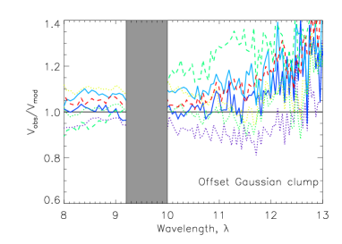


To determine if a more extended offset distribution provides a good fit to the observed visibilities, we also try to fit the data with a Gaussian clump offset from the central star. The clump is modelled in the same way as a central Gaussian clump, with FWHM mas. The clump is offset from the central source (the star is again modelled as a point source, so with uniform visibility of 1 everywhere) by a distance , with the tested range mas, and a position angle EoN. Note that we do not test the range 180–360∘EoN as the symmetry of the visibility function means that the visibilities are the same for clumps at EoN and EoN.
The best fitting clump model is for a clump of FWHM mas, offset from the star by a distance mas at a position angle of EoN. The size and offset of this best fitting clump model are comparable to the best fitting circularly symmetric Gaussian centered on the star (FWHM = 30mas). The offset of EoN would result in higher visibilities on baselines around EoN, which is what is seen in the observations on baseline 80-D2 (see Figure 15). The reduced for this best fitting model is 1.70. Although this seems at first sight like a reasonable fit, as explained for HD113766 the absolute values of reduced are likely to overstate the goodness-of-fit of the models tested here due to the over-estimation of the degrees of freedom in the model. In addition to the poorer fit, the best-fitting Gaussian clump model is a clump which encircles the star, and therefore is not a geometry which we could expect either from a circumplanetary disc or from the recent massive collision scenario suggested in Lisse et al. (2009).
4.4.1 Preferred model for HD172555
As with HD113766, the best fitting models have reduced , which is a reflection of the over-estimation of the number of degrees-of-freedom. In spite of this limitation to our interpretation of the absolute values of reduced , we can see from the relative values of reduced that the elliptical models and inclined rings provide a better fit to the data than a circularly symmetric Gaussian or clump model. This is made clearer by consideration of the function for the best fitting models. These plots are shown in Figure 18. It is clear from this plot that the elliptical Gaussian model offers a better fit than the circularly symmetric or offset clump models. We find there is no significant difference in the goodness-of-fit offered by elliptical Gaussian and inclined ring-like models. The circularly symmetric Gaussian and offset clump model offer similarly poor fits to the data from this analysis. We would expect a model with increased parameters to offer an improved fit to the data, and the fact that the offset clump model does not is reflected in the higher value of reduced .
As we have found that an elliptical or inclined disc structure offers a better fit to the data than a circularly symmetric model, we want to test the limits we can place on the inclination/ellipticity and position angle of the disc with the data. We use the elliptical Gaussian model as the simpler model to test the parameter ranges. To determine the limits on the inclination of the disc model, we sum the values over all values of the FWHM and position angle for each value of the inclination in turn. The resulting probability distribution is shown in Figure 19. Models with inclinations of and are ruled out at the 3 level according to the percentage points of the distribution by this calculation, suggesting that a moderately inclined or elliptical disc is needed to fit the visibility data. We use the same technique to determine the limits on the other model parameters (results shown in Figure 19). These tests show that discs with FWHM mas and lying at position angles EoN or EoN are also ruled out at the 3 level. This lower limit on the disc size translates to 1AU at 29.9pc.
5 Discussion
The results presented in this paper provide the most accurate direct measurement of the dust at 1–8AU around any main-sequence star. The MIDI data on HD113766 reveal a partially resolved disc. The best fitting models suggest a disc diameter of 9–12mas (1.2–1.6AU). A circularly symmetric Gaussian provides a good fit to the data which suggests we do not have significant evidence for asymmetries in the disc structure which might be expected from a recent massive collision for example. We also find no improvement in the fit if we consider elliptical Gaussians, and thus there is no evidence that the disc is inclined or that the binary is forcing an ellipticity on the disc. The binary has a spectral type of F5 and lies at a projected distance of 157AU. At this distance the binary would not be expected to have a strong influence on dust at 1.6AU (unless the binary has an extremely elliptical orbit, , Holman & Wiegert 1999). There is no evidence that this system has additional cold dust components. The Q band imaging data (which is more sensitive to cooler dust populations than the N band) puts a limit of 500mJy on cooler discs around HD113766 (see Figure 3). This limit applies to discs with radii 015 (20AU) and assume a favourable disc geometry (inclined discs or if face-on, narrow disc geometries offer the best chance of detection).
For HD172555 we find visibility functions that are compatible with completely resolved excess emission. Modelling the observed data with ring-like distributions of dust suggests that the emitting material lies at a radial offset from the star of 35mas (1AU at a parallax distance of 29.2pc). We also find tentative evidence for an inclined or elliptical disc structure, with major axis orientated at EoN. The TReCS imaging data on this target places an upper limit of 7.9AU on the extent of the disc in the N band, giving a combined constraint of 1–7.9AU on the dust’s location. The TReCS Q-band imaging also indicates the presence of a more extended component, located at 8AU from the star. This component is inclined or elliptical in structure, lying at a position angle of 110∘EoN. The N band imaging shows that the 10m emission must come from a region inside this, and from the MIDI results we infer a similar postion angle to that seen in the Q band image, but at a low significance. This suggests that the two may be linked in an extended disc, with the N and Q band data probing the inner and outer regions of the distribution respectively. However, HD 172555 may also have two spatially distinct components, similar to other multi-component discs (e.g. Tel, Smith et al. 2009a; Leo, Stock et al. 2010; Corvi, Smith et al. 2009b). HD 172555 could be viewed as another young solar system (see Tel ; Smith et al. 2009a), and so could alternatively be interpreted as having two debris belts somewhat analogous to the asteroid and Kuiper belts in the Solar System. Neither configuration rules out the recent massive collision scenario suggested by Lisse et al. (2009) for the origin of the emission. An alternative extended disc distribution could also explain the results presented in this paper, with the N and Q band data probing the inner and outer regions of the distribution respectively. Again, such a distribution does not rule out the possibility of a recent massive collision, although if the majority of the emission is believed to have arisen from a collision, dynamical models will be required to confirm that the resulting ejecta can be spread over such a wide spatial range.
The young ages of the systems studied here (16Myr and 12Myr), combined with the lack of observed cold dust in these systems and the location from which the observed emission is seen to arise all suggest we are witnessing ongoing terrestrial planet formation. Lisse et al. (2009) concluded that the spectrum of HD113766 is consistent with emission from a disrupted S-type asteroid (of km in radius) or an asteroid belt made up of a large number of small S-type asteroids. Such a belt is a natural consequence of terrestrial planet formation (see e.g., Kenyon & Bromley 2004). For HD172555 Lisse et al. (2009) suggest that the excess emission arises from a recent massive collision similar to that believed to have formed the Earth-Moon system. If this is a true model of the source of the excess then we might expect a clumpy dust distribution, however we do not see any evidence for this in the visibility functions. Wyatt & Dent (2002) presented a model for the evolution of a clump following a massive collision in a debris disc, which they found to be an unlikely source for the asymmetric dust distribution in Fomalhaut. Assuming a radius of 5.8AU, a parent planetesimal radius of 1000km with density 2.5 g cm-3 (from the fitting of Lisse et al. 2009) and a specific incident energy required for catastrophic destruction of a planetesimal =200 J kg-1, we find that the time taken for a dust cloud produced in a massive collision to occupy half the disc (and thus no longer be observable as a clump) is 200 years. As the constraints from the modelling of the IRS spectrum on the lifetime of the dust arising from a massive collision suggest that the collision should have occurred in the last 0.1Myr, clump-like emission would only be expected to have lasted for the first 0.2% of the lifetime of the emission (this is consistent with a clump lifetime of 20–30 orbital periods seen in the asteroid belt, Michel et al. 2001). It is not surprising therefore that the emission we observe is not seen to be clump-like if the origin of the emission is a massive collision. The poor fit to the observed visibilities provided by clump models suggests that we can rule out the possibility of the emission arising from circumplanetary regions (around an as yet undetected planet).
The constraints we can place on the radial location of the emitting dust around HD113766 and HD172555 with these observations are of particular interest, as when combined with spectral analysis they allow the possibility of constraining models for the dust grains themselves. This is important because predictions of the location of the debris based on spectral analyses alone can be highly dependent on assumptions made about the grain properties such as size. For HD113766, the location of the dust inferred from spectral analysis is 13mas (1.7AU Lisse et al. 2008), slightly larger than our MIDI observations imply. For HD172555 dust has been predicted to arise from a region around 5.8AU (Lisse et al., 2009), at the larger end of the 1–7.9AU scales that the MIDI and TReCS observations presented here imply. We believe these discrepancies are due to the modelling methods used, scaling observations made during the Deep Impact Temple 1 experiment to account for the luminosity of each target star. As our new interferometric data constrains the dust in both systems to be located in regions smaller than predicted from the Lisse et al. (2008) and Lisse et al. (2009) models, the implication is that the dust composition is different from the dust released in the Deep Impact event such that it would be hotter if placed at the same distance from any given star. These constraints will allow the next-generation models to treat the dust composition and location in a self-consistent way.
In this paper we have presented new VISIR spectroscopic and MIDI interferometric observations of the youngest debris disc hosts with emission on 10AU scales, HD113766 and HD172555. We have additionally presented new VISIR imaging observations of HD113766, which rule out large-scale high surface brightness emission. We find that the visibility functions measured for HD113766 are consistent with symmetric emission in the region between 0.6–0.8AU (or a diameter of 1.2–1.6AU). For HD172555 the visibility functions observed suggest that the emission is completely resolved with the VLTI, placing a lower limit of 1AU on the spatial extent of the emitting region. A new analysis of TReCS data originally presented in Moerchen et al. (2010) has revealed extended emission around HD 172555 in the Q band, consistent with an inclined disc at a median radius of 7.9AU from the star. This means that the HD172555 system could contain multiple disc components, or that we are observing different regions of a broad dust distribution around this stars in the different bands. These observations are the first that resolve the mid-infrared excess emission around these targets. In both cases the observational data are compatible with current models that suggest we are observing two systems in the midst of terrestrial planet forming processes.
Acknowledgments
Based on observations made with ESO Telescopes at the Paranal Observatories under programme IDs 078.D-0808, 079.C-0259, 080.C-0737, and 083.C-0775. The authors wish to thank Christine Chen for providing the Spitzer IRS spectra of HD113776 and HD172555.
References
- Andrae et al. (2010) Andrae R., Schulze-Hartung T., Melchior P., 2010, arXiv:1012.3754v1
- Beichman et al. (2005) Beichman C. A., et al., 2005, ApJ, 626, 1061
- Beichman et al. (2011) Beichman C. A., et al., 2011, ApJ, 743, 85
- Beichman et al. (1988) Beichman C. A., Neugebauer G., Habing H. J., Clegg P. E., Chester T. J., 1988, in Beichman C. A., Neugebauer G., Habing H. J., Clegg P. E., Chester T. J., eds, Infrared astronomical satellite (IRAS) catalogs and atlases. Volume 1: Explanatory supplement Vol. 1, Infrared astronomical satellite (IRAS) catalogs and atlases. Volume 1: Explanatory supplement
- Berger & Segransan (2007) Berger J. P., Segransan D., 2007, New Astronomy Reviews, 51, 576
- Chen et al. (2005) Chen C. H., Patten B. M., Werner M. W., Dowell C. D., Stapelfeldt K. R., Song I., Stauffer J. R., Blaylock M., Gordon K. D., Krause V., 2005, ApJ, 634, 1372
- Chen et al. (2006) Chen C. H., et al., 2006, ApJS, 166, 351
- Chesneau (2007) Chesneau O., 2007, New Astronomy Review, 51, 666
- Cohen et al. (1999) Cohen M., Walker R. G., Carter B., Hammersley P., Kidger M., Noguchi K., 1999, AJ, 117, 1864
- Cox (2000) Cox A. N., 2000, Allen’s astrophysical quantities. (New York: AIP Press; Springer)
- Dullemond & Monnier (2010) Dullemond C. P., Monnier J. D., 2010, ARAA, 48, 205
- Fujiwara et al. (2009) Fujiwara H., et al., 2009, in T. Onaka, G. J. White, T. Nakagawa, & I. Yamamura ed., Astronomical Society of the Pacific Conference Series Vol. 418 of Astronomical Society of the Pacific Conference Series, A Search for Hot Debris Disks Based on AKARI/IRC All-Sky Survey Data. pp 109–+
- Geers et al. (2007) Geers V. C., van Dishoeck E. F., Visser R., Pontoppidan K. M., Augereau J., Habart E., Lagrange A. M., 2007, A&A, 476, 279
- Gomes et al. (2005) Gomes R., Levison H. F., Tsiganis K., Morbidelli A., 2005, Nature, 435, 466
- Heng (2011) Heng K., 2011, arXiv:1104.4499
- Holman & Wiegert (1999) Holman M. J., Wiegert P. A., 1999, AJ, 117, 621
- Kenyon & Bromley (2004) Kenyon S. J., Bromley B. C., 2004, AJ, 127, 513
- Lisse et al. (2008) Lisse C. M., Chen C. H., Wyatt M. C., Morlok A., 2008, ApJ, 673, 1106
- Lisse et al. (2009) Lisse C. M., Chen C. H., Wyatt M. C., Morlok A., Song I., Bryden G., Sheehan P., 2009, ApJ, 701, 2019
- Malbet et al. (2005) Malbet F., et al., 2005, A&A, 437, 627
- Michel et al. (2001) Michel P., Benz W., Tanga P., Richardson D. C., 2001, Science, 294, 1696
- Moerchen et al. (2010) Moerchen M. M., Telesco C. M., Packham C., 2010, ApJ, 723, 1418
- Moerchen et al. (2007) Moerchen M. M., Telesco C. M., Packham C., Kehoe T. J. J., 2007, ApJL, 655, L109
- Pantin & di Folco (2011) Pantin E., di Folco E., 2011, “Mid-IR observations of the HD172555 debris disk”, Talk at EPSC-DPS Joint Meeting 2011, 02 -– 07 October 2011, Nantes, France
- Schneider et al. (2006) Schneider G., et al., 2006, ApJ, 650, 414
- Smith et al. (2009a) Smith R., Churcher L. J., Wyatt M. C., Moerchen M. M., Telesco C. M., 2009, A&A, 493, 299
- Smith & Wyatt (2010) Smith R., Wyatt M. C., 2010, A&A, 515, A95
- Smith et al. (2008) Smith R., Wyatt M. C., Dent W. R. F., 2008, A&A, 485, 897
- Smith et al. (2009b) Smith R., Wyatt M. C., Haniff C. A., 2009, A&A, 503, 265
- Song et al. (2005) Song I., Zuckerman B., Weinberger A. J., Becklin E. E., 2005, Nature, 436, 363
- Stock et al. (2010) Stock N. D., et al., 2010, ApJ, 724, 1238
- Tristram (2007) Tristram K. R. W., 2007, PhD thesis, Max-Planck-Institut für Astronomie, Königstuhl 17, 69117 Heidelberg, Germany
- Verhoelst (2005) Verhoelst T., 2005, PhD thesis, Institute of Astronomy, K.U.Leuven, Belgium
- Wahhaj et al. (2007) Wahhaj Z., Koerner D. W., Sargent A. I., 2007, ApJ, 661, 368
- Wyatt (2008) Wyatt M. C., 2008, ARAA, 46, 339
- Wyatt et al. (2010) Wyatt M. C., Booth M., Payne M. J., Churcher L. J., 2010, MNRAS, 402, 657
- Wyatt & Dent (2002) Wyatt M. C., Dent W. R. F., 2002, MNRAS, 334, 589
- Wyatt et al. (2007a) Wyatt M. C., Smith R., Greaves J. S., Beichman C. A., Bryden G., Lisse C. M., 2007, ApJ, 658, 569
- Wyatt et al. (2007b) Wyatt M. C., Smith R., Su K. Y. L., Rieke G. H., Greaves J. S., Beichman C. A., Bryden G., 2007, ApJ, 663, 365
- Zuckerman (2001) Zuckerman B., 2001, ARAA, 39, 549