Moment analysis of focus-diverse point spread functions for modal wavefront sensing of uniformly illuminated circular-pupil systems

Hanshin Lee^∗

McDonald Observatory, University of Texas at Austin, 1 University Station C1402, Austin, TX, 78712, USA
^∗Corresponding author: lee@astro.as.utexas.edu

Abstract

A new concept of using focus-diverse point spread functions (PSFs) for modal wavefront sensing (WFS) is explored. This is based on relatively straightforward image moment analysis of measured PSFs, which differentiates it from other focal-plane wavefront sensing techniques (FPWFS). The presented geometric analysis shows that the image moments are non-linear functions of wave aberration coefficients, but notes that focus-diversity (FD) essentially decouples the coefficients of interest from others, resulting in a set of linear equations whose solution corresponds to modal coefficient estimates. The presented proof-of-concept simulations suggest the potential of the concept in WFS with strongly aberrated high SNR objects in particular.

OCIS codes:  010.7350,110.2960,080.1010,120.5050,220.4840

Optical wavefront is aberrated during its passage through physical systems due to perturbations like turbulence in Earth atmosphere or misalignment of telescopes. Useful understanding of the observed behaviours of the systems can be obtained by sensing the aberration coefficients of the wavefront. Typically, a wavefront is measured at the pupil of an imaging system, as in Shack-Hartmann sensors (SHS) where wavefront slope is measured and then wave aberration is determined from the measurement[1]. It can be efficient and accurate, but requires a separete relay for pupil re-imaging with additional optical components.

In some cases, one wishes to sense wavefront across the field of view of an instrument by using the built-in components without separate relay components. Such desires can be satisfied by applying FPWFS techniques to focus-diverse images. Curvature sensing (CS) is a FPWFS method where the intensity difference between two extra-focal images are used to determine wavefront[2]. The CS signal is directly related to the shape of a membrane deformable mirror, enabling efficient control of the wavefront compensator[1]. In Phase retrieval, another FPWFS method, wavefront is optimized until its synthetic focus-diverse images closely match the measured ones[3]. It can be accurate and flexible, but may be less efficient than others due to a potentially large number-crunching during optimization. However, progress has been made to address this issue[4, 5, 6].

In this Letter, the idea of a new type of FPWFS technique is explored. Like others, it utilizes focus-diverse PSFs, but differs, in that aberrations are sensed via image moment analysis of the PSFs. The presented geometric analysis shows that the moments are non-linear functions of wave aberration coefficients, but notes that FD essentially decouples the coefficients of interest, leading to linear equations whose solution corresponds to modal coefficient estimates. It is argued that this approach has potential in WFS as shown in the presented simulations. Noll’s notations are adopted throughout[7].

Geometrically, aberrated systems spread rays around and blur their PSFs, but the blur shape uniquely differs depending on wave aberrations, e.g. comet-like PSF blur by coma (see pp. 90 in[8] for more examples). Such geometric relations can be explained by the connection between ray and wave aberrations. Suppose that a wavefront $\Phi$ on the unit-disk pupil $\Omega$ is given as,

$$\Phi=a_{1}\,Z_{1}+a_{2}\,Z_{2}+a_{3}\,Z_{3}+\cdots+a_{M}\,Z_{M},$$ (1)

where $a_{i}$ are the wave aberration coefficients and $Z_{i}$ are the Zernike polynomials in the pupil coordinates ($x,y$). The ray coordinates ($X,Y$) at the focus are given by differentiating $\Phi$ by $x$ and $y$, respectively.

$$X=X_{0}+2F\,\frac{\partial\Phi}{\partial x},\;\;Y=Y_{0}+2F\,\frac{\partial\Phi}{\partial y},$$ (2)

where ($X_{0},Y_{0}$) are the ideal image coordinates and $F$ is the focal ratio. The derivative terms are given as,

$$\begin{array}[]{c}2F\;\partial\Phi/\partial x=\vec{a}^{T}\,\mathbf{\Gamma}^{x}\,\vec{Z}={(\vec{a}{{}^{\prime}}^{x})}^{T}\,\vec{Z}\\ 2F\;\partial\Phi/\partial y=\vec{a}^{T}\,\mathbf{\Gamma}^{y}\,\vec{Z}={(\vec{a}{{}^{\prime}}^{y})}^{T}\,\vec{Z}\end{array},$$ (5)

where $\vec{a}{{}^{\prime}}^{x}$ and $\vec{a}{{}^{\prime}}^{y}$ are slope coefficient vectors and $\vec{Z}$ is the vector of $Z_{i}$. Noll noted the derivatives of $Z_{i}$ can be given in terms of $Z_{i}$ through the conversion matrices $\mathbf{\Gamma}^{x}$ and $\mathbf{\Gamma}^{y}$[7]. $a{{}^{\prime}}_{i}^{x}$ and $a{{}^{\prime}}_{i}^{y}$ are related to $a_{i}$, e.g. for $M$=10

$$a{{}^{\prime}}_{1}^{x}= 2a_{2}+2\sqrt{2}a_{8},\;\;\;\;\;a{{}^{\prime}}_{1}^{y}=2a_{3}+2\sqrt{2}a_{7},$$

$$a{{}^{\prime}}_{2}^{x}= 2\sqrt{3}a_{4}+\sqrt{6}a_{6},\;\;a{{}^{\prime}}_{2}^{y}=\sqrt{5}a_{5}+\sqrt{10}a_{13},$$

$$a{{}^{\prime}}_{3}^{x}= \sqrt{5}a_{5}+\sqrt{10}a_{13},\;a{{}^{\prime}}_{3}^{y}=2\sqrt{3}a_{4}-\sqrt{6}a_{6}$$

$$a{{}^{\prime}}_{4}^{x}= 2\sqrt{6}a_{8},\;\;\;\;\;\;\;\;\;\;\;\;\;\;\;\;\;a{{}^{\prime}}_{4}^{y}=2\sqrt{6}a_{7},$$

$$a{{}^{\prime}}_{5}^{x}= 2\sqrt{3}a_{7}+2\sqrt{3}a_{9},\;a{{}^{\prime}}_{5}^{y}=2\sqrt{3}a_{8}-2\sqrt{3}a_{10},$$

$$a{{}^{\prime}}_{6}^{x}= 2\sqrt{3}a_{8}+2\sqrt{3}a_{10},a{{}^{\prime}}_{6}^{y}=-2\sqrt{3}a_{7}+2\sqrt{3}a_{9}.$$ (6)

One way to quantify the PSF shape is computing its $k$th moment of order $k=n+m\geq 1$, that is given as,

$$\mu_{nm}=S^{-1}\int_{\Omega}I\,(X-X_{0})^{n}\,(Y-Y_{0})^{m}d\Omega,$$ (7)

where $I$ is the pupil illumination and $S$ is its integral over $\Omega$. Here, the moment is computed using the pupil plane quantities (i.e. $I$, $X$, and $Y$), whereas this is usually done using focal plane quantities. But, note that the focal plane PSF is essentially determined by the pupil plane quantities. Thus, Eq. 7 should lead to the moment as computed in the usual way.

With $I=1$ over $\Omega$, $S=\pi$ and the centroids become $\mu_{10}=a{{}^{\prime}}_{1}^{x}$ and $\mu_{01}=a{{}^{\prime}}_{1}^{y}$. Apparently, $\mu_{nm}$ with $k\geq 2$ is non-linear in $a{{}^{\prime}}_{i}^{x}$ or $a{{}^{\prime}}_{i}^{y}$, but only some slope coefficients (say $b_{i}$) are coupled to $(a{{}^{\prime}}_{2}^{x})^{\alpha}(a{{}^{\prime}}_{3}^{y})^{\beta}$ where $\alpha+\beta+1=k$. Note that $a{{}^{\prime}}_{2}^{x}$ and $a{{}^{\prime}}_{3}^{y}$ are the only coefficients affected by defocus ($a_{4}$), thus differentiating these with respect to $a_{4}$ by $k$-1 times decouples $b_{i}$ from $(a{{}^{\prime}}_{2}^{x})^{\alpha}(a{{}^{\prime}}_{3}^{y})^{\beta}$. For instance, the derivatives of $\mu_{nm}$ at $k$=2 (Eq. 8),

$$\mu_{20}=\sum_{i=2}^{M}(a{{}^{\prime}}_{i}^{x})^{2},{\mu}_{11}=\sum_{i=2}^{M}\,a{{}^{\prime}}_{i}^{x}a{{}^{\prime}}_{i}^{y},\mu_{02}=\sum_{i=2}^{M}\,(a{{}^{\prime}}_{i}^{y})^{2},$$ (8)

are the followings.

$$\frac{\partial{\mu}_{20}}{\partial a_{4}}=4\sqrt{3}a{{}^{\prime}}_{2}^{x},\frac{\partial{\mu}_{11}}{\partial a_{4}}=4\sqrt{3}a{{}^{\prime}}_{3}^{x},\frac{\partial{\mu}_{02}}{\partial a_{4}}=4\sqrt{3}a{{}^{\prime}}_{3}^{y}.$$ (9)

Note $a{{}^{\prime}}_{3}^{x}=a{{}^{\prime}}_{2}^{y}$ from Eq. 6. Another example is for $k=3$, where the 2nd partial derivatives of ${\mu}_{nm}$ are given as,

$$\frac{\partial^{2}{\mu}_{30}}{\partial{a^{2}_{4}}} =c(a{{}^{\prime}}_{4}^{x}+\sqrt{2}a{{}^{\prime}}_{6}^{x}),\frac{\partial^{2}{\mu}_{12}}{\partial{a^{2}_{4}}}=d(5a{{}^{\prime}}_{4}^{x}-3\sqrt{2}a{{}^{\prime}}_{6}^{x}),$$

$$\frac{\partial^{2}{\mu}_{03}}{\partial{a^{2}_{4}}} =c(a{{}^{\prime}}_{4}^{y}-\sqrt{2}a{{}^{\prime}}_{6}^{y}),\frac{\partial^{2}{\mu}_{21}}{\partial{a^{2}_{4}}}=d(5a{{}^{\prime}}_{4}^{y}+3\sqrt{2}a{{}^{\prime}}_{6}^{y}),$$

$$\mathrm{with} \;a{{}^{\prime}}_{5}^{x}=\sqrt{2}a{{}^{\prime}}_{4}^{y}+a{{}^{\prime}}_{6}^{y},\;a{{}^{\prime}}_{5}^{y}=\sqrt{2}a{{}^{\prime}}_{4}^{x}+a{{}^{\prime}}_{6}^{x},$$ (10)

where $c=12\sqrt{3}$ and $d=4\sqrt{3}$. Solving the above equations produces the slope coefficients. In a similar way, the $k$-1th partial derivatives of the $k$th moments can be used to estimate the slope coefficients at the $k$-1th order. The slope estimates can then be used in Eq. 5 to determine $a_{i}$ of radial order up to $k$.

What does it mean to have the derivative of moment in reality then? It is simply FD. Through-focusing is one way to achieve it, where the PSF is recorded at $N$ different intra- or extra-focal planes and the image moments of the PSFs are measured. This obviously leads to $\mu_{nm}$ that is a function of $\Delta a_{4}$. Note $N$=$k$ and $\Delta a_{4}$=$\Delta L/(16\sqrt{3}F^{2})$ in the unit of focus perturbation $\Delta L$. Finally, fitting a polynomial of degree $k$-1 to the measured $\mu_{nm}$ results in the $k$-1th coefficient that corresponds to the $k$-1th derivative of $\mu_{nm}$ with respect to $a_{4}$. In summary, one can obtain the dependence of $\mu_{nm}$ on $a{{}^{\prime}}_{i}^{x}$, $a{{}^{\prime}}_{i}^{y}$ from Eq.2, 5, 6 and the $k$-1th derivative of $\mu_{nm}$ with respect to $a_{4}$ leads to simple expressions allowing to estimate $a_{i}$. To experimentally measure the derivative, the PSF should be recorded at $k$ different image planes or FDs.

As a proof-of-concept, I demonstrate a simulation where non-zero $a_{i}$ with $i=2,3,4,\cdots,10$ are estimated by using three through-focus images sampled at -1mm, 0mm, and 1mm ($\Delta a_{4}$$\sim$$\pm 0.7\lambda$) from the ideal focus of a f/10 system with 2.7m aperture (plate scale $\sim 7.6^{\prime\prime}/mm$). A standard FFT method was used for synthesising polychromatic PSFs[9].

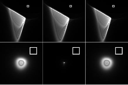
Fig. 1: Polychromatic through-focus PSFs on 512² grid with uniform spectral weight at 11 wavelengths between 514nm and 614nm, Top: Initial, Bottom: After correction, Left: -1mm before focus, Middle: at focus, Right: +1mm after focus. 50$\mu m$ squares overlaid for size comparison. Images in square-root scale.

The initial wavefront error is quite substantial amounting to 5.7$\lambda$ in rms at $\lambda$=514nm, making the through-focusing effect in the PSF shape barely noticeable. The pixel size is 5$\mu m$. The estimated coefficients are compared to the input values in Table 1. The estimated slope coefficients ($\hat{a}{{}^{\prime}}_{i}^{x}$, $\hat{a}{{}^{\prime}}_{i}^{y}$) match the true values (${a}{{}^{\prime}}_{i}^{x}$, ${a}{{}^{\prime}}_{i}^{y}$) with sub-pixel accuracy. The maximum difference between the estimated ($\hat{a}_{i}$) and the true ($a_{i}$) wave coefficients is 0.032$\lambda$ in $a_{9}$. The PSFs after applying $\hat{a}_{i}$ as corrections are in the bottom row of Figure 1.

Table 1: Slope (in pixel) and wave (in $\lambda$) coefficients in Figure 1.

$i^{k}$	$\hat{a}{{}^{\prime}}_{i}^{x}$	${a}{{}^{\prime}}_{i}^{x}$	$\hat{a}{{}^{\prime}}_{i}^{y}$	$a{{}^{\prime}}_{i}^{y}$	$\hat{a}_{i}$	$a_{i}$
10	-11.926	-11.959	-1.078	-1.144	–	–
21	-27.885	-27.986	7.956	7.968	-1.198	-1.185
31	7.956	7.968	-30.874	-31.015	1.612	1.636
42	-12.351	-12.505	-13.033	-13.316	-4.241	-4.241
52	1.823	1.766	-18.399	-18.601	1.624	1.626
62	0.932	0.917	20.255	20.598	0.305	0.309
73	–	–	–	–	-1.330	-1.359
83	–	–	–	–	-1.261	-1.276
93	–	–	–	–	1.593	1.614
103	–	–	–	–	1.392	1.408

In the next demonstration, the same images were binned by a factor of 4 (Figure 2). The same moment analysis was applied to the binned images and the resultant wave and slope aberration coefficients are compared to the true values in Table 2. The binning effectively reduces the spatial resolution of the images. This leads to a fewer pixels used in the moment analysis and thus reduces the moment measurement accuracy. To some extent, binning is equivalent to low-pass filtering, washing out small-scale diffraction structures that may not be accounted for by the geometric wavefront aberrations, although diffraction effect appears to be less of an issue in the current analysis. Overall, the binning impact seems more prominent in the coefficients with odd radial orders ($k$=$1,3$) than in the even radial order coefficients ($k$=$2$). The estimated slope coefficients still approximate the true values with sub-pixel accuracy.

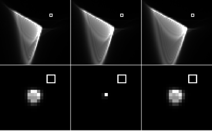
Fig. 2: Polychromatic through-focus PSFs with 4x4 binning, Top: Initial, Bottom: After correction, Left: -1mm before focus, Middle: at focus, Right: +1mm after focus. 50$\mu m$ squares overlaid for comparison. Images in square-root scale.

The maximum difference between $\hat{a}_{i}$ and $a_{i}$ is 0.032 wave in $a_{9}$. The through-focus PSFs after applying $\hat{a}_{i}$ as corrections are shown in the bottom row of Figure 2.

Table 2: Slope (in pixel) and wave (in $\lambda$) coefficients in Figure 2.

$i^{k}$	$\hat{a}{{}^{\prime}}_{i}^{x}$	${a}{{}^{\prime}}_{i}^{x}$	$\hat{a}{{}^{\prime}}_{i}^{y}$	$a{{}^{\prime}}_{i}^{y}$	$\hat{a}_{i}$	$a_{i}$
10	-11.924	-11.959	-1.080	-1.144	–	–
21	-27.851	-27.986	7.928	7.968	-1.182	-1.185
31	7.928	7.968	-30.884	-31.015	1.607	1.636
42	-12.468	-12.505	-13.006	-13.316	-4.239	-4.241
52	1.761	1.766	-18.385	-18.601	1.618	1.626
62	0.753	0.917	20.155	20.598	0.310	0.309
73	–	–	–	–	-1.328	-1.359
83	–	–	–	–	-1.273	-1.276
93	–	–	–	–	1.582	1.614
103	–	–	–	–	1.381	1.408

Finally, random aberrations (from $a_{2}$ to $a_{15}$, i.e. M=15) were applied to 21 point objects with different brightness. The aberration, without tip/tilt, amounts to 0.5$\lambda$ rms at 500nm. The images of four object are shown at the maximum FD of $1\lambda$ in the inset (Figure 3). Five FD frames were obtained, where the pixel size is 18$\mu m$ with scale of 0.15^′′ at 2.7m aperture and uniformly weighted 11 wavelengths between 500nm and 600nm were used with photon shot noise. The signal-to-noise ratio (SNR), the square root of total photons collected as computed at the zero FD, ranges from 11 to 221. The rms residual error, i.e. the root sum square of $\hat{a}_{i}-a_{i}$, is plotted against SNR (blue) with two power-law fits.

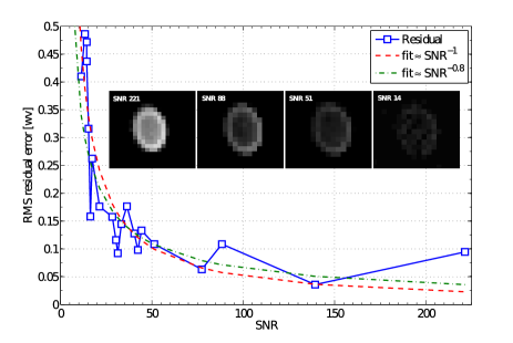
Fig. 3: Four object images at 1$\lambda$ FD (inset), RMS residual error against SNR for 21 objects.

While the green curve fits the blue data better, the red fit also asymptotes the data and follows the general behavior of the accuracy of other WFS techniques ($\sim$SNR^-1)[1]. It appears that SNR higher than 50 per frame is needed to obtain accuracy better than 0.1$\lambda$. This translates to SNR$\sim$20 for a SHS with N=30 sub-apertures, based on the requirement of 2$M$$\leq$$N$[11, 12], leading to the theoretical SHS accuracy of 0.05$\lambda$[1]. The analysis indicates the proposed technique to be suitable for high SNR cases, while spatial filtering, noise reduction, or thresh-holding could help improve its robustness in low SNR cases.

The demonstrations suggest the feasibility of the proposed geometric concept in WFS with high SNR and strong aberrations in particular. The fact that the moment analysis is just an extension of the routine computation of image centroid or full-width-half-maximum can make all appropriate objects recorded in an image frame be potential WFS targets. This can certainly permit a straightfoward and rapid WFS potentially over a wide field of view, which can be particularly attractive in active diagnosis of alignment-driven field aberrations of imaging systems[13] or wide-field adaptive image compensation. The error propagation is to be separately discussed with other considerations including aberration aliasing, diffraction, and FD implementation.

References

- [1] J. W. Hardy, Adaptive Optics for Astronomical Telescopes, (Oxford, 1998).
- [2] F. Roddier, “Wavefront sensing and the irradiance transport equation,” Appl. Opt. , 29, 1402 (1990).
- [3] J. R. Fineup, “Phase-retrieval algorithm: a comparison,” Appl. Opt. , 21, 2758 (1982).
- [4] J. Dolne, P. Menicucci, D. Miccolis, K. Widen, H. Seiden, F. Vachss, and H. Schall, ”Advanced image processing and wavefront sensing with real-time phase diversity,” Appl. Opt. 48, A30-A34 (2009).
- [5] R. Gonsalves, “Small-phase solution to the phase-retrieval problem,” Opt. Lett. 26, 684-685 (2001).
- [6] S. Meimon, T. Fusco, and L. Mugnier, “LIFT: a focal-plane wavefront sensor for real-time low-order sensing on faint sources,” Opt. Lett. 35, 3036-3038 (2010).
- [7] R.J. Noll, “Zernike polynomials and atmospheric turbulence,” J. Opt. Soc. Am., 66, 207 (1976).
- [8] V.N. Mahajan, Aberration Theory Made Simple, (SPIE, 1991).
- [9] J. W. Goodman, Introduction to Fourier Optics, 3rd ed. (Roberts & Company, 2005).
- [10] N. Roddier, “Atmospheric wavefront simulation using Zernike polynomials,” Opt. Eng. 29, 1174 (1990).
- [11] J.Y.Wang and D.E.Silva, ”Wave-front interpretation with Zernike polynomials,” Appl. Opt. , 19, 1510 (1980).
- [12] M.G. Lofdahl, A.L. Duncan, and G.B.Scharmer, ”Fast Phase Diversity Wavefront Sensing for Mirror Control,” Proc. SPIE 3353, 952 (1998).
- [13] H. Lee, “Optimal collimation of misaligned optical systems by concentering primary field aberrations,” Opt. Express 18, 19249 (2010).