Effect of charged impurity correlation on transport in monolayer and bilayer graphene

Abstract

We study both monolayer and bilayer graphene transport properties taking into account the presence of correlations in the spatial distribution of charged impurities. In particular we find that the experimentally observed sublinear scaling of the graphene conductivity can be naturally explained as arising from impurity correlation effects in the Coulomb disorder, with no need to assume the presence of short-range scattering centers in addition to charged impurities. We find that also in bilayer graphene correlations among impurities induce a crossover of the scaling of the conductivity at higher carrier densities. We show that in the presence of correlation among charged impurities the conductivity depends nonlinearly on the impurity density $n_{i}$ and can even increase with $n_{i}$.

I Introduction

The scaling of the conductivity $\sigma$ as a function of gate-voltage, proportional to the average carrier density $n$, is invaluable in characterizing the properties of graphene Novoselov et al. (2004). The functional dependence of $\sigma(n)$ at low temperatures contains information Das Sarma et al. (2011); Peres (2010) about the nature of disorder in the graphene environment (i.e., quenched charged impurity centers, lattice defectsChen et al. (2009), interface roughness Ishigami et al. (2007), ripplesKatsnelson and Geim (2008); Bao et al. (2009), resonant scattering centers Stauber et al. (2007); Monteverde et al. (2010); Wehling et al. (2010); Ferreira et al. (2011), etc.) giving rise to the dominant scattering mechanism. At finite temperatures electron-phonon scattering contributes to the resistivity Efetov and Kim (2010); Hwang and Das Sarma (2008a); Min et al. (2011). However, in graphene the electron-phonon scattering is very weak and it becomes important only at relatively high temperatures ($\gtrsim 400K$), as evidence also from the fact that around room temperature the temperature dependence of $\sigma$ appears to be dominated by activation processes Li et al. (2011a); Heo et al. (2011). The quantitative weakness of the electron-phonon interaction in graphene gives particular impetus to a thorough understanding of the disorder mechanisms limiting graphene conductivity since this may enable substantial enhancement of room temperature graphene-based device for technological applications. This is in sharp contrast to other high-mobility 2D systems such as GaAs-based devices whose room-temperature mobility could be orders of magnitude lower than the corresponding low-temperature disorder-limited mobility due to strong carrier scattering by phononsHwang and Das Sarma (2008b). Therefore, a complete understanding of the disorder mechanisms controlling $\sigma(n)$ in graphene at $T=0$ is of utmost importance both from a fundamental and a technological prospective.

The experimental study of $\sigma(n)$ in gated graphene goes back to the original discovery of 2D graphene,Novoselov et al. (2004); Novoselov et al. (2005a) and is a true landmark in the physics of electronic materials. Essentially, all experimental work on graphene begins with a characterization of $\sigma(n)$ and the mobility, $\mu=\sigma/(ne)$. A great deal is therefore known Novoselov et al. (2004); Novoselov et al. (2005a); Tan et al. (2007); Chen et al. (2008); Bolotin et al. (2008); Feldman et al. (2009) about the experimental properties of $\sigma(n)$ in graphene. The most important features of the experimentally observed $\sigma(n)$ Novoselov et al. (2005b, a); Tan et al. (2007); Chen et al. (2008); Bolotin et al. (2008); Feldman et al. (2009); Hong et al. (2009) in monolayer graphene (MLG) are: (1) a non-universal sample-dependent minimum conductivity $\sigma(n\approx 0)\equiv\sigma_{min}$ at the charge neutrality point (CNP) where the average carrier density vanishes; (2) a linearly increasing, $\sigma(n)\propto n$ , conductivity with increasing carrier density on both sides of the CNP upto some sample dependent characteristic carrier density; (3) a sublinear $\sigma(n)$ for high carrier density, making it appear that the very high density $\sigma(n)$ may be saturating.

To explain the above features of $\sigma(n)$ a model has been proposed Das Sarma et al. (2011); Adam et al. (2007); Rossi et al. (2009); Hwang et al. (2007); Ando (2006); Nomura and MacDonald (2007) with two distinct scattering mechanisms: the long-range Coulomb disorder due to random background charged impurities and static zero-range (often called “short-range”) disorder. The net graphene conductivity with these two scattering sources is then given by $\sigma\equiv\rho^{-1}=(\rho_{c}+\rho_{s})^{-1}$, where $\rho_{c}$ and $\rho_{s}$ are resistivities arising respectively from charged impurity and short-range disorder. It has been shown that Das Sarma et al. (2011); Adam et al. (2007); Rossi et al. (2009); Hwang et al. (2007); Ando (2006); Nomura and MacDonald (2007) $\rho_{c}\sim 1/n$ and $\rho_{s}\sim$ constant in graphene, leading to $\sigma(n)$ going as

$$\sigma(n)=\frac{n}{A+Cn},$$ (1)

where the density independent constants $A$ and $C$ are known Das Sarma et al. (2011) as functions of disorder parameters; $A$, arising from Coulomb disorder, depends on the impurity density ($n_{i}$) (and also weakly on their locations in space) and the background dielectric constant ($\kappa$) whereas the constant $C$, arising from the short-range disorder Das Sarma et al. (2011); Hwang et al. (2007), depends on the strength of the white-noise disorder characterizing the zero-range scattering. Eq. (1) clearly manifests the observed $\sigma(n)$ behavior of graphene for $n\neq 0$ since $\sigma(n\ll A/C)\sim n$, and $\sigma(n\gg A/C)\sim 1/C$ with $\sigma(n)$ showing sublinear $(C+A/n)^{-1}$ behavior for $n\sim A/C$.

The above-discussed scenario for disorder-limited graphene conductivity, with both long-range and short-range disorder playing important qualitative roles at intermediate $(n_{i}\lesssim n\leqslant A/C)$ and high $(n>A/C)$ carrier densities respectively, has been experimentally verified by several groups Tan et al. (2007); Chen et al. (2008); Bolotin et al. (2008); Feldman et al. (2009); Hong et al. (2009). There is, however, one serious issue with this reasonable scenario: although the physical mechanism underlying the long-range disorder scattering is experimentally established Das Sarma et al. (2011); Tan et al. (2007); Chen et al. (2008) to be the presence of unintentional charged impurity centers in the graphene environment, the physical origin of the short-range disorder scattering is unclear and has so far eluded direct imaging experiments. As a matter of fact the experimental evidence suggests that point defects (e.g. vacancies) are rare in graphene and should produce negligible short-range disorder. There have also been occasional puzzling conductivity measurements [e.g., Ref. Ponomarenko et al., 2009; Schedin et al., 2007] reported in the literature which do not appear to be explained by the standard model of independent dual scattering by long- and short-range disorder playing equivalent roles.

Recently a novel theoretical model has been proposed Li et al. (2011b) that is able to semiquantitatively explain all the major features of $\sigma(n)$ observed experimentally assuming only the presence of charged impurities. The key insight on which the model relies is the fact that in experiments, in which the samples are prepared at room temperature and are often also current annealed, it is very likely that spatial correlations are present among the charged impurities. In particular this model is able to explain the linear (sublinear) scaling of $\sigma(n)$ in MLG at low (high) $n$ without assuming the presence of short-range scattering centers.

In this work we first review the transport model proposed in Ref. [Li et al., 2011b], and then extend it to the case of bilayer graphene (BLG). We find that, as in MLG, the presence of spatial-correlations among impurities is able to explain a crossover of the scaling of $\sigma(n)$ from low $n$ to high $n$ in BLG, as observed in experiments, and that, because of the spatial correlations, $\sigma$ depends non-monotonically on the impurity density $n_{i}$.

The remainder of this paper is structured as follows. In Section II we present the model and the results for the structure factor $S({\bf q})$ that characterizes the impurity correlations. With the structure factor calculated in Sec. II we provide the transport theory in Section III and Section IV. In Section III, we study the density-dependent conductivity $\sigma(n)$ of monolayer graphene in the presence of correlated charged impurities. We calculate $\sigma(n)$ at higher carrier density using the Boltzmann transport theory. We also evaluate $\sigma(n)$ applying both Thomas-Fermi-Dirac theory Rossi and Das Sarma (2008) and effective medium theory Rossi et al. (2009) to characterize the strong carrier density inhomogeneities close to the charge neutrality point. In Section IV, we apply the Boltzmann transport theory and the effective medium theory for correlated disorder to bilayer graphene and discuss the qualitative similarities and the quantitative differences between monolayer and bilayer graphene. We briefly review the experimental situation in Section V. We then conclude in Section VI.

II Structure factor $S({\bf q})$ of Correlated disorder

In this section we describe the model used to calculate the structure factor $S({\bf q})$ for the charged impurities. We then present results for $S({\bf q})$ obtained using this model via Monte Carlo simulations. The Monte Carlo results are then used to build a simple continuum approximation for $S({\bf q})$, which captures all the features of $S({\bf q})$ that are relevant for the calculation of $\sigma(n)$.

II.1 Model for the structure factor $S({\bf q})$

To calculate $S({\bf q})$ we follow the procedure presented in Ref. Kawamura and Sarma, 1996, adapted to the case of a honeycomb structure. The approach was applied to study the effects of impurity scattering in GaAs heterojunctions and successfully explained the experimental observation of high-mobilities (e.g. greater than $10^{7}$ cm²/(V$\cdot$s)) in modulation-doped GaAs heterostructures. The possible charged impurity positions on graphene form a triangular lattice specified by $\mathbf{r}_{LM}=\mathbf{a}L+\mathbf{b}M$. The vectors $\mathbf{a}=(1,0)a_{0}$ and $\mathbf{b}=(\sqrt{3}/2,1/2)a_{0}$ defined in the x-y plane, with $a_{0}=4.92$Å, which is two times the graphene lattice constant since the most densely packed phase of impurity atoms (e.g. K as in Ref. Chen et al., 2008) on graphene is likely to be an $m\times m$ phase with $m=2$ for K Caragiu and Finberg (2005). The structure factor, including the Bragg scattering term, is given by the following equation:

$$S({\bf q})=\frac{1}{N_{i}}\langle\sum_{i,j}e^{i{\bf q}\cdot({\bf r}_{i}-{\bf r}_{j}}\rangle$$ (2)

where ${\bf r}_{i},{\bf r}_{j}$ are the random positions on the lattice $\bf r_{LM}$ of the charged impurities and the angle brackets denote averages over disorder realizations. Introducing the fractional occupation $f\equiv N_{i}/N$ of the total number of available lattice sites $N$ by the number of charged impurities $N_{i}$, and the site occupation factor $\epsilon_{LM}$ equal to 1 if site ${\bf r}_{l}$ is occupied or zero if unoccupied, we can rewrite Eq. (2) as

$$S({\bf q})=\frac{1}{f}\sum_{LM}\langle\epsilon_{LM}\epsilon_{0}\rangle e^{i{\bf q}\cdot{\bf r}_{LM}}$$ (3)

in which the sum is now over all the available lattice sites (not only the ones occupied by the impurities). By letting $C_{LM}\equiv\langle\epsilon_{LM}\epsilon_{0}\rangle/f^{2}$ we can rewrite Eq. (3) as:

$$S({\bf q})=f\sum_{LM}C_{LM}e^{i{\bf q}\cdot{\bf r}_{LM}}.$$ (4)

We then subtract the Bragg scattering term from this expression considering that it does not contribute to the resistivity obtaining

$$S({\bf q})=f\sum_{LM}(C_{LM}-1)e^{i{\bf q}\cdot{\bf r}_{LM}}.$$ (5)

It is straightforward to see that for the totally random case, the structure factor is given by $S(\mathbf{q})=1-f$ and $n_{i}\simeq 4.8f\times 10^{14}\text{cm}^{-2}$. For the correlated case we assume that two impurities cannot be closer than a given length $r_{0}<r_{i}\equiv(\pi n_{i})^{-1/2}$ defined as the correlation length. This model is motivated by the fact that two charged impurities cannot be arbitrarily close to each other because the Coulomb repulsion among the impurities during device growth and there must be a minimum separation between them.

II.2 Monte Carlo results for $S({\bf q})$

Using Monte Carlo simulations carried out on a $200\times 200$ triangular lattice with $10^{6}$ averaging runs and periodic boundary conditions we have calculated the structure factor given by Eq. (5). In the Monte Carlo calculation a lattice site is chosen randomly and becomes occupied only if it is initially unoccupied and has no nearest neighbors within the correlation length $r_{0}$. This process is repeated until the required fractional occupation for a given impurity density is obtained. Once the configuration is generated, the $C_{LM}$ can be numerically determined after doing the ensemble average. In the numerical calculations, we use only statistically significant $C_{LM}$, i.e., $|\mathbf{r}_{LM}-\mathbf{r}_{00}|\leq 3r_{0}$, since $C_{LM}$ is essential unity for $|\mathbf{r}_{LM}-\mathbf{r}_{00}|>3r_{0}$.

In Fig. 1, we present a contour plot of the structure factor $S({\bf q})$ obtained from the Monte Carlo simulations for two different values of the impurity density. For $r_{0}\neq 0$ the structure factor is suppressed at small momenta. Moreover the suppression of $S({\bf q})$ at small momenta is more pronounced, for fixed $r_{0}$, as $n_{i}$ is increased as it can be seen comparing the two panels of Fig. 1. The magnitude of $S({\bf q})$ at small ${\bf q}$ mostly determines the d.c. conductivity and therefore, from the results of Fig. 1, is evident that the presence of spatial correlations among the charged impurities will strongly affect the value of the conductivity.

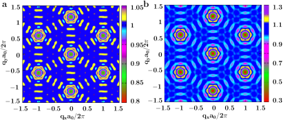
Figure 1: (a) Density plot of the structure factor $S({\bf q})$ obtained from Monte Carlo simulations for $a_{0}=4.92\;\AA$ and $r_{0}=5a_{0}$. (a) $n_{i}=0.95\times 10^{12}$ cm^-2; (b) $n_{i}=4.8\times 10^{12}$ cm^-2.

II.3 Continuum model for $S({\bf q})$

Given that the value of the d.c. conductivity depends almost entirely on the value of $S({\bf q})$ at small momenta, as discussed in Sections III and IV, it is convenient to introduce a simple continuum model being able to reproduce for small ${\bf q}$ the structure factor obtained via Monte Carlo simulations. A reasonable continuum approximation to the above discrete lattice model is given by the following pair distribution function $g({{\bf r}})$ (${{\bf r}}$ is a 2D vector in the graphene plane),

$$g({\bf r})=\begin{cases}0&|{\bf r}|\leq r_{0}\\ 1&|{\bf r}|>r_{0}\end{cases}.$$ (6)

for the impurity density distribution. In terms of the pair correlation function $g({\bf r})$ the structure factor is given by:

$$S({\bf q})=1+n_{i}\int d^{2}re^{i\mathbf{q\cdot r}}[g(\mathbf{r})-1]$$ (7)

For uncorrelated random impurity scattering, as in the standard theory, $g({\bf r})=1$ always, and $S({\bf q})\equiv 1$. With Eqs. (6) and  (7), we have

$$S(q)=1-2\pi n_{i}\frac{r_{0}}{q}J_{1}(qr_{0})$$ (8)

where $J_{1}(x)$ is the Bessel function of the first kind. Fig. 2 shows $S({\bf q})$ obtained both via Monte Carlo simulations and by using the simple continuum analytic model [Eq. (8)] for a few values of $r_{0}$ and $n_{i}$. We can see that the continuum model reproduces extremely well the dependence of the structure factor on ${\bf q}$ for small momenta, i.e. the region in momentum space that is relevant for the calculation of $\sigma$.

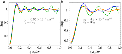
Figure 2: (a) and (b) show the calculated structure factor $S({\bf q})$ for two values of impurity density $n_{i}$. (a) $n_{i}=0.95\times 10^{12}$ cm^-2; (b) $n_{i}=4.8\times 10^{12}$ cm^-2. The solid lines show $S({\bf q})$ using Eq. (8). Dot-dashed and dashed lines show the Monte Carlo results for two different directions of ${\bf q}$ from $x$-axis, $\theta=0$ and $\theta=30^{\circ}$, respectively.

III Monolayer graphene conductivity

In this section, we explore how the spatial correlations among charged impurities affect monolayer graphene transport properties. To minimize the parameters entering the model we assume the charged impurities to be in a 2D plane placed at an effective distance $d$ from the graphene sheet (and parallel to it).

We first study the density-dependent conductivity in monolayer graphene transport for large carrier densities ($n\gg n_{i}$) using the Boltzmann transport theory, where the density fluctuations of the system can be ignored. We then discuss $\sigma(n)$ close to the charge neutrality point, where the graphene landscape breaks up into puddles Martin et al. (2008); Rossi and Das Sarma (2008); Zhang et al. (2009); Deshpande et al. (2009a); Adam et al. (2009); Deshpande et al. (2011) of electrons and holes due to the effect of the charged impurities using the effective medium theory developed in Ref.[Rossi et al., 2009].

III.1 High density: Boltzmann transport theory

Using the Boltzmann theory for the carrier conductivity at temperature $T=0$ we have

$$\sigma=\frac{e^{2}}{h}\frac{gE_{F}\tau(E_{F})}{2\hbar},$$ (9)

where $E_{F}$ is the Fermi energy, $g=4$ is the total degeneracy of graphene, and $\tau$ is the transport relaxation time at the Fermi energy obtained using the Born approximation. The scattering time at $T=0$ due to the disorder potential created by charged impurities taking into account the spatial correlations among impurities is given by Hwang and Das Sarma (2007); Li et al. (2011a); not :

$$\dfrac{\hbar}{\tau(\epsilon_{p{\bf k}})} = 2\pi n_{i}\int\dfrac{d^{2}k^{\prime}}{(2\pi)^{2}}\left[\dfrac{V(|\mathbf{k-k^{\prime}}|)}{\varepsilon(|\mathbf{k-k^{\prime}}|)}\right]^{2}S(\mathbf{k-k^{\prime}})$$ (10)

$$\times g(\theta_{\bf kk^{\prime}})\left[1-\cos\theta_{\bf kk^{\prime}}\right]\delta(\epsilon_{p\mathbf{k^{\prime}}}-\epsilon_{p\mathbf{k}})$$

where $V(q)=2\pi e^{2}/\kappa qe^{-qd}$ is the Fourier transformation of the 2D Coulomb potential created by a single charged impurity in an effective background dielectric constant $\kappa$, $\varepsilon(q)$ is the static dielectric function, $\epsilon_{s\mathbf{k}}=s\hbar v_{F}k$ is the carrier energy for the pseudospin state “$s$”, $v_{F}$ is graphene Fermi velocity, ${\bf k}$ is the 2D wave vector, $\theta_{\bf kk^{\prime}}$ is the scattering angle between in- and out- wave vectors ${\bf k}$ and ${\bf k^{\prime}}$, $g(\theta_{\bf kk^{\prime}})=\left[1+\cos\theta_{\bf kk^{\prime}}\right]/2$ is a wave function form-factor associated with the chiral nature of MLG (and is determined by its band structure). The two dimensional static dielectric function $\varepsilon(q)$ is calculated within the random phase approximation (RPA) Hwang and Das Sarma (2007), and given by

$$\varepsilon(q)=\begin{cases}1+\dfrac{4k_{F}r_{s}}{q}&\text{if\ \ }q<2k_{F}\\ 1+\dfrac{\pi r_{s}}{2}&\text{if}\ \ q>2k_{F}\end{cases}$$ (11)

After simplifying Eq. 10, the relaxation time in the presence of correlated disorder is given by:

$$\dfrac{\hbar}{\tau}=\Bigg{(}\dfrac{\pi n_{i}\text{$\hbar$}v_{F}}{4k_{F}}\Bigg{)}r_{s}^{2}\int\frac{d\theta\left(1-\cos^{2}\theta\right)}{\left(\sin\frac{\theta}{2}+2r_{s}\right)^{2}}S(2k_{F}\sin\frac{\theta}{2}),$$ (12)

where $k_{F}$ is the Fermi wavevector ($k_{F}=E_{F}/(\hbar v_{F})$), and $r_{s}$ is the graphene fine structure constant ($r_{s}=e^{2}/(\hbar v_{F}\kappa)\simeq 0.8$ for graphene on a SiO₂ substrate). For uncorrelated random impurity scattering (i.e., $r_{0}=0$, $g({\bf r})=1$, and $S({\bf q})\equiv 1$) we recover the standard formula for Boltzmann conductivity by screened random charged impurity centers Hwang et al. (2007); Ando (2006); Nomura and MacDonald (2007), where the conductivity is a linear function of carrier density.

By approximating the structure factor $S(2k_{F}\sin\theta/2)$ that appears in (12) by a Taylor expansion around $k_{F}\sin\theta/2=0$ it is possible to obtain an analytical expression for $\sigma(n)$ that allows us to gain some insight on how the spatial correlation among charged impurities affect the conductivity in MLG. Expanding the first kind of Bessel function $J_{1}(x)$ in Eq. 8 around $x\sim 0$ to the third order

$$J_{1}(x)\simeq\frac{x}{2}-\frac{x^{3}}{16}.$$ (13)

from Eq. (12) we obtain:

$$\dfrac{\hbar}{\tau}\simeq\dfrac{4\pi n_{i}\text{$\hbar$}v_{F}}{k_{F}}r_{s}^{2}\left[G_{1}(r_{s})\left(1-\pi n_{i}r_{0}^{2}\right)+G_{2}(r_{s})\dfrac{\pi n_{i}k_{F}^{2}r_{0}^{4}}{2}\right],$$ (14)

where the dimensionless functions $G_{1}(x)$ and $G_{2}(x)$ are given by, Hwang and Das Sarma (2008c)

$$\begin{array}[]{l l l }G_{1}(x)=\dfrac{\pi}{4}+6x-6\pi x^{2}+4x(6x^{2}-1)g(x),\\ \\ G_{2}(x)=\dfrac{\pi}{16}-\dfrac{4x}{3}+3\pi x^{2}+40x^{3}[1-\pi x+\dfrac{4}{5}(5x^{2}-1)g(x)],\end{array}$$ (15)

where

$$g(x)=\begin{cases}\dfrac{\text{sech}^{-1}(2x)}{\sqrt{1-4x^{2}}}&\text{if\ \ }x<\frac{1}{2},\\ \\ \dfrac{\text{sec}^{-1}(2x)}{{\sqrt{4x^{2}-1}}}&\text{if\ \ }x>\frac{1}{2}.\end{cases}$$ (16)

Using Eq. (9), (14), and recalling that $k_{F}=\sqrt{\pi n}$, we find:

$$\sigma(n)=\dfrac{An}{1-a+Ba^{2}n/n_{i}},$$ (17)

where

$$A = \dfrac{e^{2}}{h}\frac{1}{2n_{i}r_{s}^{2}G_{1}(r_{s})}$$

$$a = \pi n_{i}r_{0}^{2}$$ (18)

$$B = \frac{G_{2}(r_{s})}{2G_{1}(r_{s})}.$$

Note $a<1$ in our model because the correlation length can not exceed the average impurity distance, i.e., $r_{0}<r_{i}=(\pi n_{i})^{-1/2}$. Eq. (17) indicates that at low carrier densities the conductivity increases linearly with $n$ at a rate that increases with $r_{0}$

$$\sigma(n)\sim\dfrac{An}{(1-a)};$$ (19)

whereas at large carrier densities the dependence of $\sigma$ on $n$ becomes sublinear:

$$\sigma(n)\sim 1-\dfrac{n_{c}}{n},$$ (20)

where $n_{c}=(1-a)n_{i}/(Ba^{2})\sim O(1/n_{i}r_{0}^{4})$. Note that the above equation is valid for $\sqrt{\pi n}r_{0}\ll 1$, where we expand the structure factor as a power series of $\sqrt{\pi n}r_{0}$. The crossover density $n_{c}$, where the sublinearity ($n>n_{c}$) manifests itself, increases strongly with decreasing $r_{0}$. This generally implies that the higher mobility annealed samples should manifest stronger nonlinearity in $\sigma(n)$, since annealing leads to stronger impurity correlations (and hence larger $r_{0}$). This behavior has been observed recently in experiments in which the correlation among charged impurities was controlled via thermal annealing Yan and Fuhrer (2011). Contrary to the standard-model with no spatial correlation among charged impurities in which the resistivity increases linearly in $n_{i}$, Eq. (17) indicates that the resistivity could decrease with increasing impurity density if there are sufficient inter-impurity correlations. This is due to the fact that, for fixed $r_{0}$, higher density of impurities are more correlated causing $S({\bf q})$ to be more strongly suppressed at low $q$ as shown in Fig. 1 and 2. In the extreme case, i.e., $r_{0}=a_{0}$ and $r_{i}=r_{0}$, the charged impurity distribution would be strongly correlated, indeed perfectly periodic, and the resistance, neglecting other scattering sources, would be zero. From Eq. (17) we find that the resistivity reaches a maximum when the condition

$$r_{i}/r_{0}=\sqrt{2(1-\pi Bnr_{0}^{2})}.$$ (21)

is satisfied. Equation (21) can be used as a guide to improve the mobility of graphene samples in which charged impurities are the dominant source of disorder.

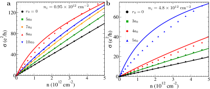
Figure 3: Calculated $\sigma(n)$ in monolayer graphene with $S({\bf q})$ obtained from the Monte Carlo simulations, symbols, and $S({\bf q})$ given by Eq. 8, solid lines for (a) $n_{i}=0.95\times 10^{12}$ cm^-2, and (b) $n_{i}=4.8\times 10^{12}$ cm^-2. The different lines correspond to different values of $r_{0}$, from top to bottom $r_{0}=10a_{0},8a_{0},7a_{0},5a_{0},0\;$ in (a) and $r_{0}=5a_{0},4a_{0},3a_{0},0\;$ in (b).

Figs. 3(a) and (b) present the results for $\sigma(n)$ obtained integrating numerically the r.h.s. of Eq. (12) and keeping the full momentum dependence of the structure factor. The solid lines show the results obtained using the $S({\bf q})$ given by the continuum model, Eq. (8), the symbols show the results obtained using the $S({\bf q})$ obtained via Monte Carlo simulations. The comparison between the two results shows that the analytic continuum correlation model is qualitatively and quantitatively reliable. It is clear that, for the same value of $r_{0}$, the dirtier (cleaner) system shows stronger nonlinearity (linearity) in a fixed density range consistent with the experimental observations Yan and Fuhrer (2011) since the correlation effects are stronger for larger values of $n_{i}$.

Fig. 4(a) presents that the resistivity $\rho=1/\sigma$ in monolayer graphene as a function of impurity density $n_{i}$ with correlation length $r_{0}=5a_{0}$ for different values of carrier density. It is clear that the impurity correlations cause a highly nonlinear resistivity as a function of impurity density and that this nonlinearity in $\rho(n_{i})$ is much stronger for lower carrier density. In Fig. 4(b) we show the value of the ratio $r_{i}/r_{0}$ for which $\rho$ is maximum as a function of $\sqrt{n}r_{0}$ The analytical expression of Eq. 21 is in very good agreement with the result obtained numerically using the full momentum dependence of $S({\bf q})$.

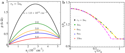
Figure 4: (a) Calculated resistivity $\rho$ in monolayer graphene as a function of impurity density $n_{i}$ for different carrier densities with $r_{0}=5a_{0}$. (b) The relationship between $r_{i}/r_{0}$ and $\sqrt{n}r_{0}$ in monolayer graphene, where the conductivity is minimum. The dashed line is obtained using Eq. 21.

III.2 Low density: Effective medium theory

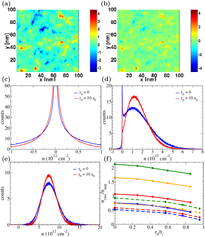
Figure 5: (color online) The carrier density in monolayer graphene for a single disorder realization obtained from the TFD theory (a) for the uncorrelated case and (b) $r_{0}=10\;a_{0}$ with $n_{i}=0.95\times 10^{12}$ cm^-2. Carrier probability distribution function $P(n)$ are shown in (c), (d), (e) for $\langle n\rangle=0$, 1.78, $7.7\times 10^{12}$ cm^-2, respectively. In (f) the ratio $n_{\rm rms}/n_{i}$ is shown as a function of $r_{0}/r_{i}$ for $n_{i}=0.95\times 10^{12}$ cm^-2, solid lines, and $n_{i}=4.8\times 10^{12}$ cm^-2, dashed lines. We use $\langle n\rangle=7.7$, 3.14, 0.94, $0\times 10^{12}$ cm^-2 for the solid lines (from top to bottom) and $\langle n\rangle=8.34$, 4.10, 1.7, $0\times 10^{12}$ cm^-2 for the dashed lines.

Due to the gapless nature of the band structure, the presence of charged impurities induce strong carrier density inhomogeneities in MLG and BLG. Around the Dirac point, the 2D graphene layer becomes a spatially inhomogeneous semi-metal with electron-hole puddles randomly located in the system. To characterize these inhomogeneities we use the Thomas-Fermi-Dirac (TFD) theory Rossi and Das Sarma (2008). Ref. [Rossi et al., 2009] has shown that the TFD theory coupled with the Boltzmann transport theory provides an excellent description of the minimum conductivity around the Dirac point with randomly distributed Coulomb impurities. We further improve this technique to calculate the density landscape and the minimum conductivity of monolayer graphene in the presence of correlated charged impurities. To model the disorder, we have assumed that the impurities are placed in a 2D plane at a distance $d=1$ nm from the graphene layer. Fig. 5(a), (b) show the carrier density profile for a single disorder realization for the uncorrelated case and correlated case ($r_{0}=10\;a_{0}$) for $n_{i}=0.95\times 10^{12}$ cm^-2. We can see that in the correlated case the amplitude of the density fluctuations is much smaller than in the uncorrelated case. The TFD approach is very efficient and allows the calculation of disorder averaged quantities such as the density root mean square, $n_{\rm rms}$, and the density probability distribution $P(n)$. Figs. 5(c), (d), (e) show $P(n)$ at the CNP, and away from the Dirac point ($n_{i}=0.95\times 10^{12}$ cm^-2). In each figure both the results for the uncorrelated case and the one for the correlated case are shown. $P(n)$ for the correlated case is in general narrower than $P(n)$ for the uncorrelated case resulting in smaller values of $n_{\rm rms}$ as shown in Fig. 5(f) in which $n_{\rm rms}/n_{i}$ as a function of $r_{0}/r_{i}$ is plotted for different values of the average density, $\langle n\rangle$, and two different values of the impurity density, $n_{i}=0.95\times 10^{12}$ cm^-2 (“low impurity density”) for the solid lines, and $n_{i}=4.8\times 10^{12}$ cm^-2 (“high impurity density”) for the dashed lines.

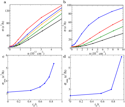
Figure 6: (a) and (b) show the results for $\sigma(\langle n\rangle)$ in monolayer graphene obtained from the EMT for $n_{i}=0.95\times 10^{12}$ cm^-2 and $n_{i}=4.8\times 10^{12}$ cm^-2 respectively. The different lines correspond to different values of $r_{0}$, from top to bottom $r_{0}=10a_{0},8a_{0},7a_{0},5a_{0},0\;$ in (a) and $r_{0}=5a_{0},4a_{0},3a_{0},0\;$ in (b). (c) and (d) show the value of $\sigma_{min}$ in monolayer graphene as a function of $r_{0}/r_{i}$.

To describe the transport properties close to the CNP and take into account the strong disorder-induced carrier density inhomogeneities we use the effective medium theory (EMT), where the conductivity is found by solving the following integral equation Bruggeman (1935); Landauer (1952, 1978); Das Sarma et al. (2011); Rossi et al. (2009); Fogler (2009); Sarma et al. :

$$\int dn\dfrac{\sigma(n)-\sigma_{EMT}}{\sigma(n)+\sigma_{EMT}}P(n)=0$$ (22)

where $\sigma(n)$ is the local Boltzmann conductivity obtained in Section III.1. Fig. 6(a) and (b) show the EMT results for $\sigma(n)$. The EMT results give similar behavior of $\sigma(n)$ at high carrier density as shown in Fig. 3, where the density fluctuations are strongly suppressed. However, close to the Dirac point, the graphene conductivity obtained using TFD-EMT approach is approximately a constant, with this constant minimum conductivity plateau strongly depending on the correlation length $r_{0}$. Fig. 6(c) and (d) show the dependence of $\sigma_{min}$ on the size of the correlation length $r_{0}$. $\sigma_{min}$ increases slowly with $r_{0}$ for $r_{0}/r_{i}<0.5$, but quite rapidly for $r_{0}/r_{i}>0.5$. The results in Fig. 6(c) and (d) are in qualitative agreement with the scaling of $\sigma_{min}$ with temperature, proportional to $r_{0}$, observed in experiments Yan and Fuhrer (2011).

IV Bilayer graphene conductivity

In this section we extend the theory presented in the previous section for monolayer graphene to bilayer graphene. MLG. The most important difference between MLG and BLG comes from the fact that, in BLG, at low energies, the band dispersion is approximately parabolic with effective mass $m\simeq 0.033m_{e}$ ($m_{e}$ being the bare electron mass) McCann et al. (2006) rather than linear as in MLG. As a consequence in BLG the scaling of the conductivity with doping, at high density, differs from the one in MLG. We restrict ourselves to the case in which no perpendicular electric field is present so that no gap is present between the conduction and the valence band Castro et al. (2007); Oostinga et al. (2008); Mak et al. (2009); Zou and Zhu (2010); Rossi and Das Sarma (2011).

To characterize the spatial correlation among charged impurities we use the same model that we used for MLG.

IV.1 High density: Boltzmann transport theory

Within the two-band approximation, the BLG conductivity at zero temperature $T=0$ is given by:

$$\sigma=\dfrac{e^{2}n\tau}{m}$$ (23)

where $\tau$ is the relaxation time in BLG for the case in which the charged impurities are spatially correlated. $\tau$ is given by Eq. 10 with $\epsilon_{s\mathbf{k}}=s\hbar^{2}k^{2}/2m$ for the pseudo-spin state “$s$”, $\epsilon(|{\bf k}-{\bf k}^{\prime}|)$ the static dielectric screening function of BLG Ref. [Hwang and Das Sarma, 2008d], and $g(\theta_{\bf kk^{\prime}})=\left[1+\cos 2\theta_{\bf kk^{\prime}}\right]/2$ the chiral factor for states on the lowest energy bands of BLG.

The full static dielectric constant of gapless BLG at $T=0$ is given by Hwang and Das Sarma (2008d)

$$\begin{array}[]{l l}\varepsilon(q)&=[1+V(q)\Pi(q)]^{-1}\\ &=[1+V(q)D_{0}\left[g(q)-f(q)\theta(q-2k_{F})\right]]^{-1}\end{array}$$ (24)

where $\Pi(q)$ is the BLG static polarizability, $D_{0}=\dfrac{2m}{\pi\hbar^{2}}$ the density of states, and

$$\begin{array}[]{l l l }f(q)&=\dfrac{2k_{F}^{2}+q^{2}}{2k_{F}^{2}q}\sqrt{q^{2}-4k_{F}^{2}}+\ln\dfrac{q-\sqrt{q^{2}-4k_{F}^{2}}}{q+\sqrt{q^{2}-4k_{F}^{2}}}\\ g(q)&=\dfrac{1}{2k_{F}^{2}}\sqrt{q^{4}+4k_{F}^{4}}-\ln\left[\dfrac{k_{F}^{2}+\sqrt{k_{F}^{4}+q^{4}/4}}{2k_{F}^{2}}\right]\end{array}$$ (25)

To make analytical progress, we calculate the density-dependent conductivity using the dielectric function of BLG within the Thomas-Fermi approximation:

$$\varepsilon(q)=1+\dfrac{q_{TF}}{q}$$ (26)

where $q_{TF}=\dfrac{4me^{2}}{\kappa\hbar^{2}}\simeq 1.0\times 10^{9}$m^-1 for bilayer graphene on $\text{SiO}_{2}$ substrate, which is a density independent constant and is larger than $2k_{F}$ for carrier density $n<8\times 10^{12}$cm^-2. The relaxation time including correlated disorder is then simplified as:

$$\dfrac{\hbar}{\tau}=\dfrac{n_{i}\pi\hbar^{2}q_{0}^{2}}{m}\int_{0}^{1}dx\left[\dfrac{1}{x+q_{0}}\right]^{2}\dfrac{x^{2}\left(1-2x^{2}\right)^{2}}{\sqrt{1-x^{2}}}S(2k_{F}x)$$ (27)

where $q_{0}=q_{TF}/(2k_{F})$. To incorporate analytically the correlation effects of charged impurities, we again expand $S(x)$ around $x\sim 0$:

$$S(2k_{F}x)\simeq 1-a+\dfrac{1}{2}\dfrac{n}{n_{i}}a^{2}x^{2}-\dfrac{1}{12}\dfrac{n^{2}}{n_{i}^{2}}a^{3}x^{4}$$ (28)

Combining Eqs. (23), (27), and (28) we obtain for $\sigma(n)$ at $T=0$ in the presence of correlated disorder

$$\sigma=\dfrac{e^{2}}{h}\dfrac{2n}{n_{i}}\frac{1}{\left[(1-a)G_{1}[q_{0}]+\frac{n}{2n_{i}}a^{2}G_{2}[q_{0}]-\frac{n^{2}}{12n_{i}^{2}}a^{3}G_{3}[q_{0}]\right]},$$ (29)

where

$$\begin{array}[]{l l l l l }G_{1}(q_{0})&=q_{0}^{2}\int_{0}^{1}\dfrac{1}{(x+q_{0})^{2}}\dfrac{x^{2}\left(1-2x^{2}\right)^{2}}{\sqrt{1-x^{2}}}dx\\ G_{2}(q_{0})&=q_{0}^{2}\int_{0}^{1}\dfrac{1}{(x+q_{0})^{2}}\dfrac{x^{4}\left(1-2x^{2}\right)^{2}}{\sqrt{1-x^{2}}}dx\\ G_{3}(q_{0})&=q_{0}^{2}\int_{0}^{1}\dfrac{1}{(x+q_{0})^{2}}\dfrac{x^{6}\left(1-2x^{2}\right)^{2}}{\sqrt{1-x^{2}}}dx\end{array}$$ (30)

For each value of $r_{0}$ and carrier density $n$, the resistivity of BLG for correlated disorder is also not a linear function of impurity density, and its behavior is close to that in MLG. The maximum resistivity of BLG is found to be at

$$r_{i}/r_{0}=\sqrt{2(1-\pi B_{B}\pi nr_{0}^{2}-C_{B}\pi^{2}n^{2}r_{0}^{4})}.$$ (31)

with $B_{B}=G_{2}[q_{0}]/(2G_{1}[q_{0}])$ and $C_{B}=-G_{3}[q_{0}]/(12G_{1}[q_{0}])$, which are functions weakly depending on carrier density $n$.

It is straightforward to calculate the asymptotic density dependence of BLG conductivity from the above formula and we will discuss $\sigma(n)$ in the strong ($q_{0}\gg 1$) and weak $q_{0}\ll 1$ screening limits separately.

In the strong screening limit $q_{0}\gg 1$, $G_{1}[q_{0}]\simeq\pi/8$, $G_{2}[q_{0}]\simeq 7\pi/64$ and $G_{3}[q_{0}]\simeq 13\pi/128$. For randomly distributed charged impurity, we can express the conductivity as a linear function of carrier density $\sigma(n)\sim n$ Das Sarma et al. (2010). In the presence of correlated charged impurity we find:

$$\sigma(n)=\dfrac{A_{B}n}{1-a+a^{2}\dfrac{7n}{16n_{i}}+a^{3}\dfrac{13n^{2}}{192n^{2}_{i}}},$$ (32)

where $a=\pi n_{i}r_{0}^{2}$, and $A_{B}\simeq\dfrac{e^{2}}{h}\dfrac{16}{\pi n_{i}}$. In the strong screening limit $q_{0}\gg 1\Rightarrow n\ll n_{i}$ from (32) we obtain $\sigma(n)\sim A_{B}n/(1-a)$. With the increase of carrier density, the calculated conductivity in BLG also shows the sublinear behavior as in MLG due to the third and fourth terms in the denominator of Eq. 32.

In the weak screening limit, $q_{0}\ll 1$, we have $G_{1}[q_{0}]\simeq\pi q_{0}^{2}/4$, $G_{2}[q_{0}]\simeq\pi q_{0}^{2}/8$ and $G_{3}[q_{0}]\simeq 7\pi q_{0}^{2}/64$. The conductivity of BLG in the limit $q_{0}\ll 1$ is a quadratic function of carrier density for randomly distributed Coulomb disorder:

$$\sigma(n)=\dfrac{e^{2}}{h}\dfrac{32n^{2}}{n_{i}q^{2}_{TF}}$$ (33)

For the correlated disorder, the calculated conductivity of BLG shows the sub-quadratic behavior:

$$\sigma(n)=\dfrac{A_{b}n^{2}}{1-a+a^{2}\dfrac{n}{4n_{i}}-a^{3}\dfrac{7n^{2}}{192n^{2}_{i}}},$$ (34)

with $A_{b}=\dfrac{e^{2}}{h}\dfrac{32}{n_{i}q^{2}_{TF}}$.

In Figs. 7(a) and (b), we show the $\sigma(n)$ within Boltzmann transport theory obtained numerically taking into account the screening via the static dielectric function given by Eq. 24. We show the results for several different correlation lengths $r_{0}$ and two different charged impurity densities, (a) $n_{i}=0.95\times 10^{12}$ cm^-2 and (b) $n_{i}=4.8\times 10^{12}$ cm^-2. From Figs. 7(a), (b) we see that the conductivity increases with $r_{0}$ as in MLG. However the details of the scaling of $\sigma$ with doping differ between MLG and BLG. In BLG $\sigma(n)\approx n^{\alpha}$ where $1<\alpha<2$ also depends on $n$. The effect of spatial correlations among impurities in BLG is to increase $\alpha$ at low densities and reduce it at high densities.

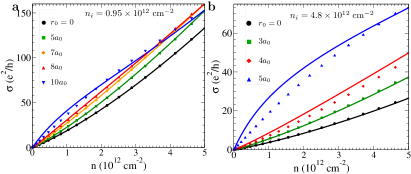
Figure 7: Calculated $\sigma(n)$ in bilayer graphene with $S({\bf q})$ obtained from the Monte Carlo simulations (symbols) and $S({\bf q})$ given by Eq. (8) (solid lines) for two different impurity densities (a) $n_{i}=0.95\times 10^{12}$ cm^-2 and (b) $n_{i}=4.8\times 10^{12}$ cm^-2. The different lines correspond to different values of $r_{0}$. In (a) we use $r_{0}=10a_{0},\;8a_{0},\;7a_{0},\;5a_{0},\;0$ (from top to bottom), and in (b) $r_{0}=5a_{0},\;4a_{0},\;3a_{0},\;0$ (from top to bottom).

In Fig. 8(a), we present the resistivity of BLG as a function of impurity density for various carrier density with $r_{0}=5a_{0}$. The spatial correlation of charged impurity leads to a highly non-linear function of $\rho(n_{i})$ as in MLG. We also present the relation between $r_{i}/r_{0}$ and $\sqrt{n}r_{0}$ where the maximum resistivity of BLG occurs in Fig. 8(b). The results are quite close to those of MLG shown in Fig. 4.

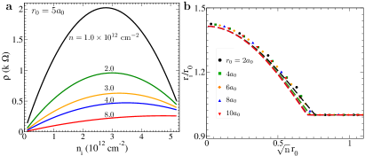
Figure 8: (a) The resistivity $\rho$ in bilayer graphene is shown as a function of impurity density $n_{i}$ for different carrier densities with $r_{0}=5a_{0}$. (b) The relationship between $r_{i}/r_{0}$ and $\sqrt{n}r_{0}$ in bilayer graphene, where the conductivity is minimum. The dashed lines are obtained using Eq. 31.

IV.2 Low density: Effective medium theory

As in MLG, also in BLG, because of the gapless nature of the dispersion the presence of charged impurities induces large carrier density fluctuations Adam and Das Sarma (2008); Deshpande et al. (2009b); Das Sarma et al. (2010); Rossi and Das Sarma (2011) that strongly affect the transport properties of BLG.

Fig. 9(a) shows the calculated density landscape for BLG for a single disorder realization, and Fig. 9(a) a comparison of the probability distribution function $P(n)$ for BLG and MLG Das Sarma et al. (2010). Within the Thomas-Fermi approximation, approximating the low energy bands as parabolic, in BLG, with no spatial correlation between charged impurities, $P(n)$ is a Gaussian whose root mean square is independent of the doping and is given by the following equation Rossi and Das Sarma (2011):

$$n_{\rm rms}=\frac{\sqrt{n_{i}}}{r_{\rm sc}}\left[\frac{2}{\pi}f(d/r_{\rm sc})\right]^{1/2}$$ (35)

where $f(d/r_{\rm sc})=e^{2d/r_{\rm sc}}(1+2d/r_{\rm sc})\Gamma(0,2d/r_{\rm sc})-1$ is a dimensionless function, $r_{\rm sc}\equiv[(2e^{2}m^{*})/(\kappa\hbar^{2})]^{-1}\approx 2$ nm is the screening length, and $\Gamma(a,x)$ is the incomplete gamma function. For small $d/r_{\rm sc}$, $f=-1-\gamma-\log(2d/r_{\rm sc})+O(d/r_{\rm sc})$ (where $\gamma=0.577216$ is the Euler constant), whereas for $d\gg r_{\rm sc}$ $f=1/(2d/r_{\rm sc})^{2}+O((d/r_{\rm sc})^{-3})$. As for MLG, also for BLG we find that the presence of spatial correlations among impurities has only a minor quantitative effect on $P(n)$. For this reason, and the fact that with no correlation between the impurities, $P(n)$ has a particularly simple analytical expression, for BLG we neglect the effect of impurity spatial correlations on $P(n)$.

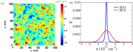
Figure 9: (Color online). (a) $n({\bf r})$ of BLG at the CNP for a single disorder realization with $n_{i}=10^{11}{\rm cm}^{-2}$ and $d=1$ nm. (b) Disorder averaged $P(n)$, at the CNP for BLG (MLG) red (blue) for $n_{i}=10^{11}{\rm cm}^{-2}$ and $d=1$ nm. For MLG $P(n=0)\approx 0.1$, out of scale. The corresponding $n_{\rm rms}$ is $5.5\times 10^{11}{\rm cm}^{-2}$ for BLG and $1.2\times 10^{11}{\rm cm}^{-2}$ for MLG.

As in MLG the effect of the strong carrier density inhomogeneities on transport can be effectively taken into account using the effective medium theory. Using Eq. (22), $\sigma(n)$ given by the Boltzmann theory, and $P(n)$ as described in the previous paragraph, the effective conductivity $\sigma_{EMT}$ for BLG can be calculated taking into account the presence of strong carrier density fluctuations. Fig. 10(a) shows the scaling of $\sigma$ with doping obtained using the EMT for several values of $r_{0}$ and $n_{i}=4.8\times 10^{12}$ cm^-2. Taking account of the carrier density inhomogeneities that dominates close to the charge neutrality point, the EMT returns a non-zero value of the conductivity $\sigma_{\rm min}$ for zero average density, a value that depends on the impurity density and their spatial correlations. In particular, as shown in Fig. 10(b), in analogy to the MLG case $\sigma_{\rm min}$ grows with $r_{0}$.

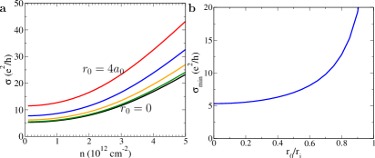
Figure 10: (a) BLG conductivity as a function of $n$ obtained using the EMT for $n_{i}=4.8\times 10^{12}$ cm^-2 for $r_{0}=(4,3,2,1,0)\times a_{0}$ from top to bottom. (b) BLG $\sigma_{\rm min}$ as a function of $r_{0}/r_{i}$ for $n_{i}=4.8\times 10^{12}$ cm^-2.

V Discussion of experiments

Although the sublinearity of $\sigma(n)$ can be explained by including both long- and short-range scatterers (or resonant scatterers) in the Boltzmann transport theory Das Sarma and Hwang (2011), it can not explain the observed enhancement of conductivity with increasing annealing temperatures as observed in Ref. [Yan and Fuhrer, 2011]. Annealing leads to stronger correlations among the impurities since the impurities can move around to equilibrium sites. Our results show that by increasing $r_{0}$, at low densities, both the conductivity and the mobility of MLG and BLG increase. Moreover, our results for MLG Li et al. (2011b) show that as $r_{0}$ increases the crossover density at which $\sigma(n)$ from linear becomes sublinear decreases. All these features have been observed experimentally for MLG Yan and Fuhrer (2011). In addition, our transport theory based on the correlated impurity model also gives a possible explanation for the observed strong nonlinear $\sigma(n)$ in suspended graphene Bolotin et al. (2008); Feldman et al. (2009) where the thermal/current annealing is used routinely. No experiment has so far directly studied the effect of increasing the spatial correlations among charged impurities in BLG and tested our predictions for BLG.

Although we have used a minimal model for impurity correlations, using a single correlation length parameter $r_{0}$, which captures the essential physics of correlated impurity scattering, it should be straightforward to improve the model with more sophisticated correlation models if experimental information on impurity correlations becomes available Yan and Fuhrer (2011). Intentional control of spatial charged impurity distributions or by rapid thermal annealing and quenching, should be a powerful tool to further increase mobility in monolayer and bilayer graphene devicesYan and Fuhrer (2011).

VI Conclusions

In summary, we provide a novel physically motivated explanation for the observed sublinear scaling of the graphene conductivity with density at high dopings by showing that the inclusion of spatial correlations among the charged impurity locations leads to a significant sublinear density dependence in the conductivity of MLG in contrast to the strictly linear-in-density graphene conductivity for uncorrelated random charged impurity scattering. We also show that the spatial correlation of charged impurity will also enhance the mobility of BLG. The great merit of our theory is that it eliminates the need for an ad hoc zero-range defect scattering mechanism which has always been used in the standard model of graphene transport in order to phenomenologically explain the high-density sublinear behavior $\sigma(n)$ of MLG. Even though the short-range disorder is not needed to explain the sublinear behavior of $\sigma(n)$ in our model we do not exclude the possibility of short range disorder scattering in real MLG samples, which would just add as another resistive channel with constant resistivity. Our theoretical results are confirmed qualitatively by the experimental measurements presented in Ref. [Yan and Fuhrer, 2011] in which the spatial correlations among charged impurities were modified via thermal annealing with no change of the impurity density. Our results, combined with the experimental observation of Ref. [Yan and Fuhrer, 2011], demonstrate that in monolayer and bilayer graphene samples in which charged impurities are the dominant source of scattering the mobility can be greatly enhanced by thermal/current annealing processes that increase the spatial correlations among the impurities.

VII Acknowledgements

This work is supported by ONR-MURI and NRI-SWAN. ER acknowledges support from the Jeffress Memorial Trust, Grant No. J-1033. ER and EHH acknowledge the hospitality of KITP, supported in part by the National Science Foundation under Grant No. PHY11-25915, where part of this work was done. Computations were carried out in part on the SciClone Cluster at the College of William and Mary.

References

- Novoselov et al. (2004) K. S. Novoselov, A. K. Geim, S. V. Morozov, D. Jiang, Y. Zhang, S. V. Dubonos, I. V. Grigorieva, and A. A. Firsov, Science 306, 666 (2004).
- Das Sarma et al. (2011) S. Das Sarma, S. Adam, E. H. Hwang, and E. Rossi, Rev. Mod. Phys. 83, 407 (2011).
- Peres (2010) N. M. R. Peres, Rev. Mod. Phys. 82, 2673 (2010).
- Chen et al. (2009) J.-H. Chen, W. G. Cullen, C. Jang, M. S. Fuhrer, and E. D. Williams, Phys. Rev. Lett. 102, 236805 (2009).
- Ishigami et al. (2007) M. Ishigami, J. H. Chen, W. G. Cullen, M. S. Fuhrer, and E. D. Williams, Nano Letters 7, 1643 (2007).
- Katsnelson and Geim (2008) M. I. Katsnelson and A. K. Geim, Phil. Trans. R. Soc. A 366, 195 (2008).
- Bao et al. (2009) W. Bao, F. Miao, Z. Chen, H. Zhang, W. Jang, C. Dames, and C. N. Lau, Nature Nanotech. 4, 562 (2009).
- Stauber et al. (2007) T. Stauber, N. M. R. Peres, and F. Guinea, Phys. Rev. B 76, 205423 (2007).
- Monteverde et al. (2010) M. Monteverde, C. Ojeda-Aristizabal, R. Weil, K. Bennaceur, M. Ferrier, S. Guéron, C. Glattli, H. Bouchiat, J. N. Fuchs, and D. L. Maslov, Phys. Rev. Lett. 104, 126801 (2010).
- Wehling et al. (2010) T. O. Wehling, S. Yuan, A. I. Lichtenstein, A. K. Geim, and M. I. Katsnelson, Phys. Rev. Lett. 105, 056802 (2010).
- Ferreira et al. (2011) A. Ferreira, J. Viana-Gomes, J. Nilsson, E. R. Mucciolo, N. M. R. Peres, and A. H. Castro Neto, Phys. Rev. B 83, 165402 (2011).
- Efetov and Kim (2010) D. K. Efetov and P. Kim, Phys. Rev. Lett. 105, 256805 (2010).
- Hwang and Das Sarma (2008a) E. H. Hwang and S. Das Sarma, Phys. Rev. B 77, 115449 (2008a).
- Min et al. (2011) H. Min, E. H. Hwang, and S. Das Sarma, Phys. Rev. B 83, 161404 (2011).
- Li et al. (2011a) Q. Li, E. H. Hwang, and S. Das Sarma, Phys. Rev. B 84, 115442 (2011a).
- Heo et al. (2011) J. Heo, H. J. Chung, S.-H. Lee, H. Yang, D. H. Seo, J. K. Shin, U.-I. Chung, S. Seo, E. H. Hwang, and S. Das Sarma, Phys. Rev. B 84, 035421 (2011).
- Hwang and Das Sarma (2008b) E. H. Hwang and S. Das Sarma, Phys. Rev. B 77, 235437 (2008b).
- Novoselov et al. (2005a) K. S. Novoselov, A. K. Geim, S. V. Morozov, D. Jiang, M. I. Katsnelson, I. V. Grigorieva, S. V. Dubonos, and A. A. Firsov, Nature 438, 197 (2005a).
- Tan et al. (2007) Y.-W. Tan, Y. Zhang, K. Bolotin, Y. Zhao, S. Adam, E. H. Hwang, S. Das Sarma, H. L. Stormer, and P. Kim, Phys. Rev. Lett. 99, 246803 (2007).
- Chen et al. (2008) J.-H. Chen, C. Jang, S. Adam, M. S. Fuhrer, E. D. Williams, and M. Ishigami, Nature Phys. 4, 377 (2008).
- Bolotin et al. (2008) K. Bolotin, K. Sikes, Z. Jiang, M. Klima, G. Fudenberg, J. Hone, P. Kim, and H. Stormer, Solid State Commun. 146, 351 (2008).
- Feldman et al. (2009) B. E. Feldman, J. Martin, and A. Yacoby, Nature Phys. 5, 889 (2009).
- Novoselov et al. (2005b) K. S. Novoselov, D. Jiang, F. Schedin, T. J. Booth, V. V. Khotkevich, S. V. Morozov, and A. K. Geim, Proc. Natl. Acad. Sci. USA 102, 10451 (2005b).
- Hong et al. (2009) X. Hong, K. Zou, and J. Zhu, Phys. Rev. B 80, 241415 (2009).
- Adam et al. (2007) S. Adam, E. H. Hwang, V. M. Galitski, and S. D. Sarma, Proc. Natl. Acad. Sci. USA 104, 18392 (2007).
- Rossi et al. (2009) E. Rossi, S. Adam, and S. Das Sarma, Phys. Rev. B 79, 245423 (2009).
- Hwang et al. (2007) E. H. Hwang, S. Adam, and S. Das Sarma, Phys. Rev. Lett. 98, 186806 (2007).
- Ando (2006) T. Ando, J. Phys. Soc. Jpn. 75, 074716 (2006).
- Nomura and MacDonald (2007) K. Nomura and A. H. MacDonald, Phys. Rev. Lett. 98, 076602 (2007).
- Ponomarenko et al. (2009) L. A. Ponomarenko, R. Yang, T. M. Mohiuddin, M. I. Katsnelson, K. S. Novoselov, S. V. Morozov, A. A. Zhukov, F. Schedin, E. W. Hill, and A. K. Geim, Phys. Rev. Lett. 102, 206603 (2009).
- Schedin et al. (2007) F. Schedin, A. K. Geim, S. V. Morozov, E. W. Hill, P. Blake, M. I. Katsnelson, and K. S. Novoselov, Nature Materials 6, 652 (2007).
- Li et al. (2011b) Q. Li, E. H. Hwang, E. Rossi, and S. Das Sarma, Phys. Rev. Lett. 107, 156601 (2011b).
- Rossi and Das Sarma (2008) E. Rossi and S. Das Sarma, Phys. Rev. Lett. 101, 166803 (2008).
- Kawamura and Sarma (1996) T. Kawamura and S. D. Sarma, Solid State Communications 100, 411 (1996).
- Caragiu and Finberg (2005) M. Caragiu and S. Finberg, J. Phys.: Condens. Matter 17, R995 (2005).
- Martin et al. (2008) J. Martin, N. Akerman, G. Ulbricht, T. Lohmann, J. H. Smet, K. von Klitzing, and A. Yacobi, Nature Physics 4, 144 (2008).
- Zhang et al. (2009) Y. Zhang, V. W. Brar, C. Girit, A. Zettl, and M. F. Crommie, Nat. Phys. 5, 722 (2009).
- Deshpande et al. (2009a) A. Deshpande, W. Bao, F. Miao, C. N. Lau, and B. J. LeRoy, Phys. Rev. B 79, 205411 (2009a).
- Adam et al. (2009) S. Adam, E. Hwang, E. Rossi, and S. D. Sarma, Solid State Communications 149, 1072 (2009).
- Deshpande et al. (2011) A. Deshpande, W. Bao, Z. Zhao, C. N. Lau, and B. J. LeRoy, Phys. Rev. B 83, 155409 (2011).
- Hwang and Das Sarma (2007) E. H. Hwang and S. Das Sarma, Phys. Rev. B 75, 205418 (2007).
- (42) For densities below the value of the conductivity obtained using the Boltzmann theory depends very weakly on ( changes by less than 10% in going from to nm) and therefore in the remainder we set d=0 to simplify the analytical expressions for the relaxation time and , see also Ref. Das Sarma et al., 2011.
- Hwang and Das Sarma (2008c) E. H. Hwang and S. Das Sarma, Phys. Rev. B 77, 195412 (2008c).
- Yan and Fuhrer (2011) J. Yan and M. S. Fuhrer, Phys. Rev. Lett. 107, 206601 (2011).
- Bruggeman (1935) D. A. G. Bruggeman, Ann. Physik 416, 636 (1935).
- Landauer (1952) R. Landauer, J. Appl. Phys. 23, 779 (1952).
- Landauer (1978) R. Landauer, in Electrical transport and optical properties of inhomogeneous media., edited by J. C. Garland and D. B. Tanner (1978), p. 2.
- Fogler (2009) M. M. Fogler, Phys. Rev. Lett. 103, 236801 (2009).
- (49) S. D. Sarma, E. H. Hwang, and Q. Li, arXiv:1109.0988 (2011).
- McCann et al. (2006) E. McCann, K. Kechedzhi, V. I. Fal’ko, H. Suzuura, T. Ando, and B. Altshuler, Phys. Rev. Lett. 97, 146805 (2006).
- Castro et al. (2007) E. V. Castro, K. S. Novoselov, S. V. Morozov, N. M. R. Peres, J. M. B. L. dos Santos, J. Nilsson, F. Guinea, A. K. Geim, and A. H. C. Neto, Phys. Rev. Lett. 99, 216802 (2007).
- Oostinga et al. (2008) J. B. Oostinga, H. B. Heersche, X. Liu, A. F. Morpurgo, and L. M. K. Vandersypen, Nat. Mater. 7, 151 (2008).
- Mak et al. (2009) K. F. Mak, C. H. Lui, J. Shan, and T. F. Heinz, Phys. Rev. Lett. 102, 256405 (2009).
- Zou and Zhu (2010) K. Zou and J. Zhu, Phys. Rev. B 82, 081407 (2010).
- Rossi and Das Sarma (2011) E. Rossi and S. Das Sarma, Phys. Rev. Lett. 107, 155502 (2011).
- Hwang and Das Sarma (2008d) E. H. Hwang and S. Das Sarma, Phys. Rev. Lett. 101, 156802 (2008d).
- Das Sarma et al. (2010) S. Das Sarma, E. H. Hwang, and E. Rossi, Phys. Rev. B 81, 161407 (2010).
- Adam and Das Sarma (2008) S. Adam and S. Das Sarma, Phys. Rev. B 77, 115436 (2008).
- Deshpande et al. (2009b) A. Deshpande, W. Bao, Z. Zhao, C. N. Lau, and B. J. LeRoy, Appl. Phys. Lett. 95, 243502 (2009b).
- Das Sarma and Hwang (2011) S. Das Sarma and E. H. Hwang, Phys. Rev. B 83, 121405 (2011).