Modelling non-linear redshift-space distortions in the galaxy clustering pattern: systematic errors on the growth rate parameter

Abstract

We investigate the ability of state-of-the-art redshift-space distortions models for the galaxy anisotropic two-point correlation function $\xi(r_{\perp},r_{\parallel})$, to recover precise and unbiased estimates of the linear growth rate of structure $f$, when applied to catalogues of galaxies characterised by a realistic bias relation. To this aim, we make use of a set of simulated catalogues at $z=0.1$ and $z=1$ with different luminosity thresholds, obtained by populating dark-matter haloes from a large N-body simulation using halo occupation prescriptions. We examine the most recent developments in redshift-space distortions modelling, which account for non-linearities on both small and intermediate scales produced respectively by randomised motions in virialised structures and non-linear coupling between the density and velocity fields. We consider the possibility of including the linear component of galaxy bias as a free parameter and directly estimate the growth rate of structure $f$. Results are compared to those obtained using the standard dispersion model, over different ranges of scales. We find that the model of Taruya et al. (2010), the most sophisticated one considered in this analysis, provides in general the most unbiased estimates of the growth rate of structure, with systematic errors within $\pm 4\%$ over a wide range of galaxy populations spanning luminosities between $L>L^{*}$ and $L>3L^{*}$. The scale-dependence of galaxy bias plays a role on recovering unbiased estimates of $f$ when fitting quasi non-linear scales. Its effect is particularly severe for most luminous galaxies, for which systematic effects in the modelling might be more difficult to mitigate and have to be further investigated. Finally, we also test the impact of neglecting the presence of non-negligible velocity bias with respect to mass in the galaxy catalogues. This can produce an additional systematic error of the order of $1-3\%$ depending on the redshift, comparable to the statistical errors the we aim at achieving with future high-precision surveys such as Euclid.

1 Introduction

The structure in the Universe grows through the competing effects of universal expansion and gravitational instability. For this reason, the large-scale spatial distribution and dynamics of galaxies, which follows in some way those of mass, provide fundamental information about the expansion history and the nature of gravity. In general, galaxies are biased tracers of the underlying mass distribution. However, they are sensitive to the same gravitational potential and their motions keep an imprint of the rate of structure growth. One manifestation of this is the observed anisotropy between the clustering of galaxies along the line-of-sight and that perpendicular to it in redshift space. These anisotropies or distortions are caused by the line-of-sight component of galaxy peculiar velocities affecting the observed galaxy redshifts from which distances are measured. In turn, the large-scale coherent component of galaxy peculiar motions is the fingerprint of the growth rate of structure.

By mapping the large-scale structure over scales which retain this primordial information, galaxy spectroscopic surveys have become one of the most powerful probes of the cosmological model. A specific application of spectroscopic surveys involves recovering cosmological information on the expansion history $H(z)$, by measuring the shape of the power spectrum (e.g. Tegmark et al. 2004; Cole et al. 2005; Percival et al. 2007; Reid et al. 2010) and tracking the baryonic acoustic oscillations (BAO) feature in the power spectrum or in the two-point correlation function at different redshifts (e.g Eisenstein et al. 2005; Percival et al. 2010; Kazin et al. 2010; Blake et al. 2011b; Anderson et al. 2012, and references therein). However, measurements of $H(z)$ alone, either from BAO or Type Ia supernovae, cannot discriminate dark energy from modifications of General Relativity (e.g. Carroll et al. 2004), in order to explain the observed recent acceleration of the expansion of the Universe (Riess et al. 1998; Perlmutter et al. 1999). This degeneracy can be lifted by measuring the growth rate at different epochs (Peacock et al. 2006; Albrecht et al. 2006). Indeed, scenarios with similar expansion history but different gravity or type of dark energy will have a different rate of structure growth resulting from different effective gravity strength in action. This makes redshift-space distortions measured from large spectroscopic surveys a very efficient probe to test cosmology, at the same level as BAO and cosmological microwave background (CMB) anisotropies. In fact, although this effect is known since the late eighties (Kaiser 1987), its usefulness as a probe of dark energy and modified gravity has been realised only recently (Guzzo et al. 2008).

Measuring the growth rate of structure from redshift-space distortions is however non trivial. The linear theory formalism for the power spectrum was first derived by Kaiser (1987) (see Hamilton 1992, for its configuration-space counterpart). Its validity is however limited to very large scales as it lacks a description of small-scale non-linear fluctuations. This model has been extended to quasi- and non-linear scales in the early nineties using the earlier ideas of the “streaming model” (Peebles 1980), in which the linear correlation function is convolved along the line-of-sight with a pairwise velocity distribution (Fisher et al. 1994; Peacock & Dodds 1994). This enables one to approximately reproduce the Fingers-of-God small-scale elongation (Jackson 1972). Fitting functions calibrated on simulations have also been proposed for this purpose (Hatton & Cole 1999; Tinker et al. 2006). Such extension of the linear model, usually referred as the “dispersion model”, has been extensively used to measure the growth rate of structure $f$ or the distortion parameter $\beta=f/b_{L}$ from redshift surveys, using measurements of both redshift-space correlation function (Peacock et al. 2001; Hawkins et al. 2003; Zehavi et al. 2005; Ross et al. 2007; Okumura et al. 2008; Guzzo et al. 2008; da Ângela et al. 2008; Cabré & Gaztañaga 2009a, b; Samushia et al. 2011b) and power spectrum (Percival et al. 2004; Tegmark et al. 2004, 2006; Blake et al. 2011a). We refer the reader to Hamilton (1998) for a review of older studies. Although generally the dispersion model is found to be a good fit on linear and quasi-linear scales (Percival & White 2009; Blake et al. 2011a), it breaks down in the non-linear regime (Taruya et al. 2010; Okumura & Jing 2011). In particular, it has been shown that it introduces systematic errors of about $10-15\%$ on the growth rate parameter (e.g. Taruya et al. 2010; Okumura & Jing 2011; Bianchi et al. 2012), of the order of or greater than the statistical errors expected from on-going and prospected very large spectroscopic surveys such as WiggleZ (Drinkwater et al. 2010), GAMA (Driver et al. 2011), VIPERS (Guzzo et al. 2012), BOSS (White et al. 2011), Euclid (Laureijs et al. 2011), or BigBOSS (Schlegel et al. 2011). In particular, Euclid, the recently selected ESA dark energy mission, should be able to constrain the growth rate at the percent level (Wang et al. 2010; Samushia et al. 2011a; Majerotto et al. 2012). There is therefore a strong need to go beyond the dispersion model, in order to bring systematic errors below this expected level of precision, i.e. measure the growth rate parameter in an unbiased way. This is particularly crucial to be able to disentangle different models of gravity. For instance, modified-gravity models with Dark Matter-Dark Energy time-dependent or constant coupling predict variations from General Relativity on the growth rate smaller than $10\%$ (Guzzo et al. 2008).

Work in this direction started since quite some time, concentrating first on describing the redshift-space clustering and dynamics of dark matter. Scoccimarro (2004) demonstrated that the dispersion model gives rise to unphysical distributions of pairwise velocities and proposed an ansatz that accounts, to some extent, for the non-linear coupling between the velocity and the density fields. This latter model has been shown to provide a better match to the observed redshift-space power spectrum in dark matter simulations (Scoccimarro 2004; Jennings et al. 2011) and has later on been refined by Taruya et al. (2010). Further approaches have also been proposed while completing this paper (Seljak & McDonald 2011; Reid & White 2011; Cai & Bernstein 2012), but we shall not discuss them in this analysis.

All mentioned advanced redshift-space distortions models have been tested so far only on the redshift-space power spectra of dark matter and dark matter haloes, as extracted from large N-body simulations (Kwan et al. 2012; Reid & White 2011; Okumura et al. 2012; Nishimichi & Taruya 2011). This is quite different from a real survey, in which the most useful tracers of mass, the galaxies, are in general biased with respect to the underlying density field through a bias which is generally non-linear and scale-dependent. The performance of redshift-space distortions models applied to galaxy populations with a priori unknown biases, has to be precisely investigated. This is the aim of this paper, in which we confront non-linear models of redshift-space distortions for the anisotropic two-point correlation function in the case of realistic galaxy samples. This is done in the framework of the concordant $\Lambda CDM$ cosmological model. We study the ability of these models to recover the linear growth rate of structure and their range of applicability. Furthermore we investigate the effects of galaxy non-linear spatial and velocity biases and quantify how the latter affect the estimated linear growth rate for differently biased galaxy populations.

The paper is organised as follows. In Sect. 2, we present the redshift-space distortions formalism and how models can be implemented in practice. In Sect. 3, we present the comparison between the different models and study the effect of galaxy non-linear bias. In Sect. 4, we investigate the impact of neglecting galaxy velocity bias in the modelling. In Sect. 5, we summarise our results and conclude.

2 Redshift-space distortions theory

2.1 Fourier space

The peculiar velocity $\mn@boldsymbol{v}$ alters objects apparent comoving position $\mn@boldsymbol{s}$ from their true comoving position $\mn@boldsymbol{r}$, as

$$\mn@boldsymbol{s}=\mn@boldsymbol{r}+\frac{v_{\parallel}(\mn@boldsymbol{r})\mn@boldsymbol{\hat{e}_{\parallel}}}{aH(a)},$$ (1)

where $H(a)$ is the Hubble parameter, $a$ is the scale factor, and $\mn@boldsymbol{\hat{e}_{\parallel}}$ is the line-of-sight unit vector. The redshift-space density field $\delta^{s}(\mn@boldsymbol{s})$ can be obtained from the real-space one by requiring mass conservation, i.e. $\left[1+\delta^{s}(\mn@boldsymbol{s})\right]d^{3}\mn@boldsymbol{s}=\left[1+\delta(\mn@boldsymbol{r})\right]d^{3}\mn@boldsymbol{r}$, as

$$\delta^{s}(\mn@boldsymbol{s})=\left[1+\delta(\mn@boldsymbol{r})\right]\left|\frac{d^{3}\mn@boldsymbol{s}}{d^{3}\mn@boldsymbol{r}}\right|^{-1}-1.$$ (2)

In the following we shall work in the plane-parallel approximation and in this limit, the Jocobian of the real- to redshift-space transformation can be simply written as,

$$\left|\frac{d^{3}\mn@boldsymbol{s}}{d^{3}\mn@boldsymbol{r}}\right|=1-f\partial_{\parallel}u_{\parallel},$$ (3)

where we defined $u_{\parallel}(\mn@boldsymbol{r})=-v_{\parallel}(\mn@boldsymbol{r})/(faH(a))$ with $f$ being the linear growth rate. The linear growth rate parameter is defined as the logarithmic derivative of the linear growth factor $D(a)$ and given by $f(a)=d\ln{D}/d\ln{a}$. To a very good approximation it has a generic form (Wang & Steinhardt 1998; Linder 2005),

$$f(a)\simeq\Omega_{m}(a)^{\gamma}$$ (4)

where

$$\Omega_{m}(a)=\frac{\Omega_{m,0}}{a^{3}}\frac{H_{0}^{2}}{H^{2}(a)}.$$ (5)

In this parametrisation, while $\Omega_{m}$ characterises the mass content in the Universe, the exponent $\gamma$ directly relates to the theory of gravity (e.g. Linder 2004). General Relativity scenarios have $\gamma\simeq 0.55$.

From Eq. 2 and Eq. 3, one can write the redshift-space density field as,

$$\delta^{s}(\mn@boldsymbol{s})=\left(\delta(\mn@boldsymbol{r})+f\partial_{\parallel}u_{\parallel}\right)\left(1-f\partial_{\parallel}u_{\parallel}\right)^{-1}.$$ (6)

One usually assumes an irrotational velocity field for which $u_{\parallel}(\mn@boldsymbol{r})=\partial_{\parallel}\Delta^{-1}\theta(\mn@boldsymbol{r})$ and where $\theta(\mn@boldsymbol{r})=\mn@boldsymbol{\nabla}\cdot\mn@boldsymbol{v}(\mn@boldsymbol{r})$ is the velocity divergence field and $\Delta$ denotes the Laplacian. In that case Eq. 6 can be recast,

$$\delta^{s}(\mn@boldsymbol{s})=\left(\delta(\mn@boldsymbol{r})+f\partial_{\parallel}^{2}\Delta^{-1}\theta(\mn@boldsymbol{r})\right)\left(1-f\partial_{\parallel}^{2}\Delta^{-1}\theta(\mn@boldsymbol{r})\right)^{-1}.$$ (7)

In Fourier space, it is noticeable that $\partial_{\parallel}^{2}\Delta^{-1}=(k_{\parallel}/k)^{2}=\mu^{2}$ with $\mu$ being the cosine of the angle between the line-of-sight and the separation vector. Therefore, one can write the redshift-space density field (Scoccimarro et al. 1999) as,

$$\delta^{s}(k,\mu) ={}\int\frac{d^{3}\mn@boldsymbol{s}}{(2\pi)^{3}}e^{-i\mn@boldsymbol{k}\cdot\mn@boldsymbol{s}}\delta^{s}(\mn@boldsymbol{s})$$ (8)

$$={}\int\frac{d^{3}\mn@boldsymbol{r}}{(2\pi)^{3}}e^{-i\mn@boldsymbol{k}\cdot\mn@boldsymbol{r}}e^{-ikf\mu}[\delta(\mn@boldsymbol{x})+\mu^{2}f\theta(\mn@boldsymbol{x})]$$ (9)

and the redshift-space power spectrum as,

$$P^{s}(k,\mu) ={}\int\frac{d^{3}\mn@boldsymbol{r}}{(2\pi)^{3}}e^{-i\mn@boldsymbol{k}\cdot\mn@boldsymbol{r}}\left<e^{-ikf\mu\Delta u_{\parallel}}\times\right.$$

$$\left.[\delta(\mn@boldsymbol{x})+\mu^{2}f\theta(\mn@boldsymbol{x})][\delta(\mn@boldsymbol{x}^{\prime})+\mu^{2}f\theta(\mn@boldsymbol{x}^{\prime})]\right>$$ (10)

where in the latter equation, $\Delta u_{\parallel}=u_{\parallel}(\mn@boldsymbol{x})-u_{\parallel}(\mn@boldsymbol{x}^{\prime})$ and $\mn@boldsymbol{r}=\mn@boldsymbol{x}-\mn@boldsymbol{x}^{\prime}$. The redshift-space power spectrum given in Eq. 10 is almost exact, the only approximation which has been done is to assume that all object line-of-sight separations are parallel. This approximation is valid for samples with pairs covering angles typically lower than $10^{\circ}$ (Matsubara 2000). Eq. 10 captures all the different regimes of distortions. While the terms in square brackets describe the squashing effect or “Kaiser effect” which leads to an enhancement of clustering on large scales due to the coherent infall of mass towards overdensities, the exponential prefactor is responsible to some extent for the Fingers-of-God effect (FoG, Jackson 1972) which disperses objects along the line-of-sight due to random motions in virialised structures. Scoccimarro (2004) proposed a simple ansatz for the redshift-space anisotropic power spectrum by making the assumption that the exponential prefactor and the term involving the density and velocity fields can be separated in the ensemble average. In that case Eq. 10 simplifies to,

$$P^{s}(k,\mu)=e^{-(fk\mu\sigma_{v})^{2}}\left[P_{\mathrm{\delta\delta}}(k)+2\mu^{2}fP_{\mathrm{\delta\theta}}(k)+\mu^{4}f^{2}P_{\mathrm{\theta\theta}}(k)\right],$$ (11)

where $P_{\mathrm{\delta\delta}}$, $P_{\mathrm{\delta\theta}}$, $P_{\mathrm{\theta\theta}}$ are respectively the non-linear mass density-density, density-velocity divergence, and velocity divergence-velocity divergence power spectra and $\sigma_{v}$ is the pairwise velocity dispersion defined as,

$$\sigma^{2}_{v}=\frac{1}{6\pi^{2}}\int P_{\mathrm{\theta\theta}}(k)dk.$$ (12)

It is found that this model captures most of the distortion features predicted by N-body simulations (Scoccimarro 2004; Jennings et al. 2011) although it breaks down in the non-linear regime (Percival & White 2009; Taruya et al. 2010). Note that in the linear regime where $P_{\mathrm{\delta\delta}}=P_{\mathrm{\delta\theta}}=P_{\mathrm{\theta\theta}}=P$ and in the limit where $k\sigma_{v}$ tends to zero, one recovers the original Kaiser (1987) formula,

$$P^{s}(k,\mu)=[1+2\mu^{2}f+\mu^{4}f^{2}]P(k),$$ (13)

derived from linear-order calculations.

In principle, the exponential prefactor and the term involving the density and velocity fields in Eq. 10, which we will refer to as the damping and Kaiser terms in the following, cannot be treated separately. Additional terms may arise in Eq. 11 from the coupling between the exponential prefactor and the velocity divergence and density fields. Taruya et al. (2010) proposed an improved model that takes into account these couplings, adding two correction terms $C_{A}$ and $C_{B}$ to Scoccimarro (2004)’s formula such as,

$$P^{s}(k,\mu) ={}D(k\mu\sigma_{v})\left[P_{\mathrm{\delta\delta}}(k)+2\mu^{2}fP_{\mathrm{\delta\theta}}(k)+\mu^{4}f^{2}P_{\mathrm{\theta\theta}}(k)\right.$$

$$\left.+C_{A}(k,\mu;f)+C_{B}(k,\mu;f)\right],$$ (14)

whose perturbative expressions are given in their appendix A. In the improved model, the exponential prefactor has been replaced by an arbitrary functional form $D(k\mu\sigma_{v})$ for which $\sigma_{v}$ is an effective pairwise velocity dispersion parameter that can be fitted for. Taruya et al. (2010) showed that while adopting a Gaussian or a Lorentzian for the damping function and letting $\sigma_{v}$ free, one improves dramatically the fit to the redshift-space power spectrum in large dark matter simulations, particularly on translinear scales.

The function $D(k\mu\sigma_{v})$ damps the power spectra in the Kaiser term but also partially mimics the effects of the pairwise velocity distribution (PVD) in virialised systems, which translate into the FoG seen in the anisotropic power spectrum and correlation function on small scales. This is analogous to the phenomenological dispersion model proposed in the early nineties (e.g. Fisher et al. 1994; Peacock & Dodds 1994) in which the linear Kaiser model in configuration space (Hamilton 1992) is radially convolved with a PVD model to reproduce the FoG elongation on small scales, as for the early streaming model (Peebles 1980).

There is however not any simple general functional form for the PVD that matches all scales for all types of tracers. The shape of the PVD is found to depend on galaxy physical properties and halo occupation (Li et al. 2006; Tinker et al. 2006), and its associated pairwise velocity dispersion to vary with scale, in particular at small separations (e.g. Hawkins et al. 2003; Cabré & Gaztañaga 2009b). It can be shown mathematically that the PVD is in fact not a single function but rather an infinite number of PVD corresponding to different scales and angles between velocities and separation vectors (Scoccimarro 2004). In practice however, the use of an exponential distribution, a Gaussian or other forms with more degrees of freedom (e.g. Tang et al. 2011; Kwan et al. 2012) shows to be very useful to fit the residual small-scale distortions remaining once the large-scale Kaiser distortions are accounted for, unless one is interested in modelling the very small highly non-linear scales.

2.2 Configuration space

The redshift-space anisotropic two-point correlation function can be obtained by Fourier-transforming the anisotropic redshift-space power spectrum as,

$$\xi(r_{\perp},r_{\parallel})=\int\frac{d^{3}\mn@boldsymbol{k}}{(2\pi)^{3}}e^{i\mn@boldsymbol{k}\cdot\mn@boldsymbol{s}}P^{s}(k,\mu)=\sum_{l}\xi^{s}_{l}(s)L_{l}(\nu)$$ (15)

where $\nu=r_{\parallel}/s$, $r_{\perp}=\sqrt{s^{2}-r_{\parallel}^{2}}$, and $L_{l}$ denote Legendre polynomials. The correlation function multipole moments $\xi^{s}_{l}(s)$ are defined as,

$$\xi^{s}_{l}(s)=i^{l}\int\frac{dk}{2\pi^{2}}k^{2}P^{s}_{l}(k)j_{l}(ks),$$ (16)

where $j_{l}$ denotes the spherical Bessel functions and

$$P^{s}_{l}(k)=\frac{2l+1}{2}\int_{-1}^{1}d\mu P^{s}(k,\mu)L_{l}(\mu).$$ (17)

In practice, it can be convenient to write the redshift-space two-point correlation function as a convolution between the Fourier transform of the damping function $D$ and that of the Kaiser term as,

$$\xi(r_{\perp},r_{\parallel}) ={}\hat{D}(r_{\parallel},\sigma_{v})\otimes\int\frac{d^{3}\mn@boldsymbol{k}}{(2\pi)^{3}}e^{i\mn@boldsymbol{k}\cdot\mn@boldsymbol{s}}P_{K}^{s}(k,\mu)$$

$$={}\hat{D}(r_{\parallel},\sigma_{v})\otimes\xi_{K}\left(r_{\perp},r_{\parallel}\right)$$

$$={}\hat{D}(r_{\parallel},\sigma_{v})\otimes\sum_{l}\xi^{s,K}_{l}(s)L_{l}(\nu)$$ (18)

In the case of the model of Eq. 11, the three non-null correlation function multipole moments related to the Kaiser term are given by,

$$\xi^{s,K}_{0}(s) ={}\xi_{\mathrm{\delta\delta}}(r)+f\frac{2}{3}\xi_{\mathrm{\delta\theta}}(r)+f^{2}\frac{1}{5}\xi_{\mathrm{\theta\theta}}(r),$$ (19)

$$\xi^{s,K}_{2}(s) ={}f\frac{4}{3}\xi^{(2)}_{\delta\theta}(r)+f^{2}\frac{4}{7}\xi^{(2)}_{\theta\theta}(r),$$ (20)

$$\xi^{s,K}_{4}(s) ={}f^{2}\frac{8}{35}\xi^{(4)}_{\theta\theta}(r),$$ (21)

where $\xi_{\mathrm{\delta\delta}}$, $\xi_{\mathrm{\delta\theta}}$, $\xi_{\mathrm{\theta\theta}}$ are the Fourier conjugate pairs of $P_{\mathrm{\delta\delta}}$, $P_{\mathrm{\delta\theta}}$, $P_{\mathrm{\theta\theta}}$ and (Hamilton 1992; Cole et al. 1994),

$$\xi^{(2)}_{X}(r) ={}\xi_{X}(r)-\frac{3}{r^{3}}\int_{0}^{r}\xi_{X}(r^{\prime})r^{\prime 2}dr^{\prime}$$ (22)

$$\xi^{(4)}_{X}(r) ={}\xi_{X}(r)+\frac{5}{2}\frac{3}{r^{3}}\int_{0}^{r}\xi_{X}(r^{\prime})r^{\prime 2}dr^{\prime}$$

$$-\frac{7}{2}\frac{5}{r^{5}}\int_{0}^{r}\xi_{X}(r^{\prime})r^{\prime 4}dr^{\prime}.$$ (23)

The correlation function multipole moments of the Kaiser term in the case of the model of Eq. 14 are given in Appendix A. For the latter model we restrain ourselves to use only the first three non-null multipole moments, as those of orders $l=6$ and $l=8$ are very poorly defined in our simulated galaxy catalogues.

2.3 From mass to galaxies

The models derived in the previous section apply in the case of perfectly unbiased tracers of mass. Real galaxies however are biased with respect to mass. Galaxy biasing is generally expected to be non-linear, scale-dependent, stochastic, and to depend on galaxy type, although it is still poorly constrained by observations. On large scales in the linear regime, one expects the bias to be a constant multiplicative factor to the mass density field as $\delta_{g}=b_{L}\delta$. In that case, it is convenient to replace the growth rate $f$ in the models with a “effective” growth rate (or distortion parameter) $\beta=f/b_{L}$, which accounts for the large-scale linear bias $b_{L}$ of the considered galaxies. This simple model is valid on large scales where the bias asymptotes to a constant value but breaks down on small non-linear scales, where bias possibly varies with scale. Recently, Okumura & Jing (2011) showed that the scale-dependent behaviour of halo bias can strongly affect the recovery of the growth rate. While some analytical approaches have been proposed to include bias non-linearity in the model (Desjacques & Sheth 2010; Matsubara 2011), here we follow a different route and assume that the scale dependence of bias is known. In fact, the latter can be measured to some extent from the data themselves in configuration space, once the shape for the underlying non-linear mass power spectrum is assumed. General arguments may suggest that galaxy motions are also biased with respect to the mass velocity field, while observations tend to indicate that this bias is small (Tinker et al. 2006; Skibba et al. 2011). In this analysis we will neglect the galaxy velocity bias in the models but discuss and quantify its impact on the recovery of $f$ in Section 4.

2.4 Constructing the galaxy redshift-space distortion models

We will use in this analysis different combinations of Kaiser terms, damping functions, and bias prescriptions. Although we will work in configuration space, we refer to the different models in this section as their Fourier-space counterpart for clarity. All the models we consider take the general form,

$$P_{g}^{s}(k,\mu)=D(k\mu\sigma_{v})P_{K}(k,\mu,b)$$ (24)

where,

$$D(k\mu\sigma_{v})=\left\{\begin{array}[]{lcl}\exp(-(k\mu\sigma_{v})^{2})\\ \\ 1/(1+(k\mu\sigma_{v})^{2})\end{array}\right.$$ (28)

and,

$$P_{K}(k,\mu,b)=\hskip 113.81102pt$$

$$\left\{\begin{array}[]{lcl}b^{2}(k)P_{\mathrm{\delta\delta}}(k)+2\mu^{2}fb(k)P_{\mathrm{\delta\delta}}(k)+\mu^{4}f^{2}P_{\mathrm{\delta\delta}}(k)\;\;\;\;{\rm(mod.~{}A)}\\ \\ b^{2}(k)P_{\mathrm{\delta\delta}}(k)+2\mu^{2}fb(k)P_{\mathrm{\delta\theta}}(k)+\mu^{4}f^{2}P_{\mathrm{\theta\theta}}(k)\;\;\;\;{\rm(mod.~{}B)}\\ \\ b^{2}(k)P_{\mathrm{\delta\delta}}(k)+2\mu^{2}fb(k)P_{\mathrm{\delta\theta}}(k)+\mu^{4}f^{2}P_{\mathrm{\theta\theta}}(k)\\ +C_{A}(k,\mu;f,b)+C_{B}(k,\mu;f,b)\;\;\;\;\;\;\;\;\;\;\;\;\;\;\;\;\;\;\;\;\;\;\;\;\;{\rm(mod.~{}C)}\end{array}\right.$$ (35)

$$b(k)=\left\{\begin{array}[]{lcl}b_{L}\\ \\ b_{L}b_{NL}(k)\end{array}\right.\;\;.$$ (39)

Hereafter, we will refer as the different $P_{K}$ models to A, B, and C. Model A corresponds to the Kaiser (1987) model with the non-linear power spectrum instead of the linear one. It assumes a linear coupling between the density and velocity fields such that $\delta\propto\theta$. Model B is the generalisation proposed by Scoccimarro (2004) that accounts for the non-linear coupling between the density and velocity fields, making explicitly appearing the velocity divergence auto-power spectrum and density–velocity divergence cross-power spectrum. Finally, model C is an extension of model B that contains the two additional correction terms proposed by Taruya et al. (2010) to correctly account for the coupling between the Kaiser and damping terms. Besides, we will consider two deterministic galaxy biasing prescriptions: a constant linear bias $b(k)=b_{L}$ and a general non-linear bias which we define as $b(k)=\left(P_{gg}/P_{\mathrm{\delta\delta}}\right)^{1/2}(k)=b_{L}b_{NL}(k)$, where $P_{gg}$ is the galaxy power spectrum and $b_{NL}(k)$ is the scale-dependent part of the bias that tends to unity at small $k$. We note that the Gaussian and Lorentzian damping forms that we will consider here, correspond respectively to Gaussian and exponential functions in configuration-space.

The redshift-space distortions models necessitate $P_{\mathrm{\delta\delta}}$, $P_{\mathrm{\delta\theta}}$, and $P_{\mathrm{\theta\theta}}$ real-space power spectra as input. These can be obtained analytically using perturbation theory. Although standard perturbation theory does not describe well the shape of these power spectra on intermediate and non-linear scales, improved treatments such as Renormalised Perturbation Theory (RPT, Crocce & Scoccimarro 2006) or Closure Theory (Taruya et al. 2009) have been shown to be much more accurate (see Carlson et al. 2009, for a thorough comparison). In particular, Closure Theory predictions are found to match large N-body simulation real-space power spectra to the percent-level up to $k=0.2$ for $z>0.5$ (Taruya et al. 2009).

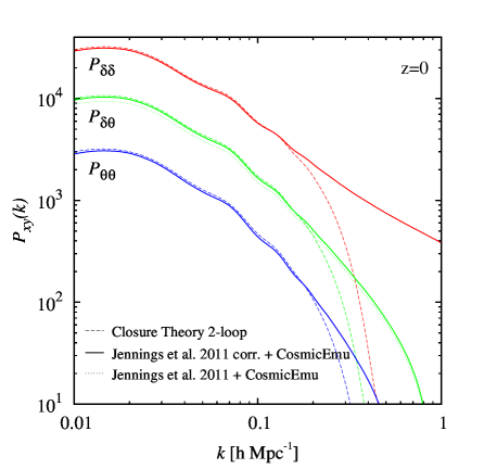
Figure 1: The predicted $P_{\mathrm{\delta\delta}}$, $P_{\mathrm{\delta\theta}}$, $P_{\mathrm{\theta\theta}}$ by CosmicEmu (Lawrence et al. 2010) and Jennings et al. (2011) fitting functions (solid and dotted curves), and Closure theory (Taruya et al. 2009) (dashed curves) at $z=0$ in the assumed cosmology. In all cases, $P_{\mathrm{\delta\theta}}$ and $P_{\mathrm{\theta\theta}}$ have been divided by a factor of 3 and 10 respectively to improve the clarity of the figure.

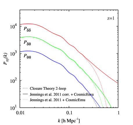
Figure 2: Same as Fig. 1 but for $z=1$.

In this analysis we use the $P_{\mathrm{\delta\delta}}$ provided by CosmicEmu emulator (Lawrence et al. 2010) and the fitting functions of Jennings et al. (2011) to obtain $P_{\mathrm{\theta\theta}}$ and $P_{\mathrm{\delta\theta}}$ from $P_{\mathrm{\delta\delta}}$. The latter fitting functions have an accuracy of $5\%$ to $k=0.2$ for both standard $\Lambda CDM$ and quintessence dark energy cosmological models. In Fig. 1 and 2 we compare the $P_{\mathrm{\delta\delta}}$, $P_{\mathrm{\delta\theta}}$, $P_{\mathrm{\theta\theta}}$ obtained in this way with Closure Theory 2-loop analytical predictions at $z=0$ and $z=1$. We find that all power spectra agree very well below $k\simeq 0.2$ and $k\simeq 0.3$ respectively for the two redshifts considered, except in the case of $P_{\mathrm{\delta\theta}}$ for which they systematically differ by about $10\%$. While all other power spectra match on linear scales, the $P_{\mathrm{\delta\theta}}$ fitting formula from Jennings et al. (2011) stays somewhat below (dotted lines in the figures). We find that by multiplying the latter by a factor of $1.1$ one obtains a good match with Closure Theory predictions on both linear and non-linear scales (solid lines in the figures). We will then adopt this correcting factor in the following when calculating the redshift-space distortions models.

It is noticeable that Closure Theory breaks down at lower $k$ than Jennings et al. (2011) fitting functions, indicating that the latter are more suitable in practice to describe clustering on the smallest scales. It is however important to mention that the validity of these fitting functions is limited at large $k$ ($k_{max}=0.2-0.3$, Jennings et al. 2011). One can therefore reliably describe the models involving $P_{\mathrm{\delta\theta}}$ and $P_{\mathrm{\theta\theta}}$ only down to scales of $r\simeq\pi/k_{max}\simeq 10.5~{}{\rm h}^{-1}~{}\rm{Mpc}$. On smaller scales, $P_{\mathrm{\delta\theta}}$ and $P_{\mathrm{\theta\theta}}$ configuration-space counterparts, $\xi_{\mathrm{\delta\theta}}$ and $\xi_{\mathrm{\theta\theta}}$, will drop rapidly and their contributions to the redshift-space distortions models will be underestimated with respect to that of $\xi_{\mathrm{\delta\delta}}$.

3 Model testing

3.1 Methodology

To test the redshift-space distortions models presented in section 2.4 and quantify how well the linear growth rate parameter $f$ can be recovered from the anisotropic two-point correlation function $\xi(r_{\perp},r_{\parallel})$, we constructed a set of realistic galaxy catalogues. We populate the identified friends-of-friends haloes in the MultiDark Run 1 (MDR1) dark matter N-body simulation (Prada et al. 2011) with galaxies by specifying the Halo Occupation Distribution (HOD). MDR1 assumes a $\Lambda CDM$ cosmology with $(\Omega_{m}=\Omega_{dm}+\Omega_{b},~{}\Omega_{\Lambda},~{}\Omega_{b},~{}h,~{}n,~{}\sigma_{8})=(0.27,~{}0.73,~{}0.0469,~{}0.7,~{}0.95,~{}0.82)$ and probe a cubic volume of $1~{}{\rm h}^{-3}~{}{\rm Gpc}^{3}$ with a mass resolution of $m_{p}=8.721\times 10^{9}~{}\rm{h^{-1}}~{}\rm{M_{\odot}}$. From haloes at snapshots $z=0.1$ and $z=1$, we built galaxy catalogues based on the current most accurate observations of the halo occupation (HOD) available at these redshifts (Zheng et al. 2007; Zehavi et al. 2011; Coupon et al. 2012) and create three luminosity-threshold samples corresponding to $L>L^{*}$, $L>2L^{*}$, and $L>3L^{*}$. In these catalogues, the redshift-space displacements with respect to real space were reproduced using Eq. 1 and the galaxy peculiar velocity information. Consistently with model assumptions, we used the plane-parallel approximation and applied redshift-space distortions along one dimension of the simulation boxes only. The details of the procedure used to create the galaxy catalogues are given in Appendix B. The main limitation of using HOD for this study rely on the hypothesis of halo sphericity and isotropy. These assumptions can have an influence on the dynamics of galaxies inside haloes, in particular on their random velocities. However, these have only a very limited impact on this analysis which focuses on scales greater than $1$$\,{\rm h}^{-1}$ Mpc, where the effect of possible anisotropies in the galaxy velocity distribution in haloes is only marginal.

We measured the anisotropic two-point auto-correlation function $\xi(r_{\perp},r_{\parallel})$ in the redshift-space catalogues using the Landy & Szalay (1993) estimator in linearly-spaced bins of $0.5{\rm h}^{-1}~{}\rm{Mpc}$ in both $r_{\perp}$ and $r_{\parallel}$ directions. Because of the large number of galaxies and to keep the computational time reasonable, all pair counts have been performed using a specifically developed parallel kd-tree code following the dual-tree approach (Moore et al. 2001).

The best-fitting parameters for the different models have been determined by adopting the usual likelihood function,

$$-2\ln{\mathcal{L}}=\sum_{i=1}^{N_{p}}\sum_{j=1}^{N_{p}}\Delta_{i}C^{-1}_{ij}\Delta_{j}$$ (40)

where $N_{p}$ is the number of points in the fit, $\Delta$ is the data-model difference vector, and $C$ is the covariance matrix of the data. The likelihood is performed on the quantity $y=\ln\left(1+\xi(r_{\perp},r_{\parallel})\right)$, rather than simply $\xi(r_{\perp},r_{\parallel})$, as to enhance the weight on large more linear scales (see Bianchi et al. 2012, for discussion).

The determination of the covariance matrix is however troublesome when fitting two-dimensional correlation functions. Having only one realisation of the simulated catalogues at each redshift, we can use to this end internal estimators, such as blockwise bootstrap or jackknife resampling (e.g. Norberg et al. 2009). Using the latter method, we find that the maximum number of cubic sub-volumes that can be extracted without underestimating the variances on the scales of interest is 64. This poses a problem, since in order to have a proper estimation of the eigenvalues of the covariance matrix, this number should be at least equal to the number of degrees of freedom, which in our case ranges between 14397 and 25597 (i.e. $120^{2}$ to $160^{2}$ data points minus $3$ free parameters) depending on the scale interval of the fit. As a result, the covariance matrix estimated in this way is degenerate and in the end not very useful. We note that this is a general problem for redshift-space distortions analysis, when one tries to fit the full anisotropic two-point correlation function or power spectrum. In principle this could be solved by using a very large number of realisations or alternatively, theoretically-motivated analytical forms for the covariance matrix. In our case, due to the limited size of the simulation, it is impracticable to define more sub-volumes than degrees of freedom, as this would result in underestimating the covariances by using too small sub-volumes. We note however that by estimating $\xi(r_{\perp},r_{\parallel})$ using bins of size $0.5{\rm h}^{-1}~{}\rm{Mpc}$ in both directions in the jackknife resamplings, we are oversampling the functions so the actual number of degrees of freedom may be smaller than that associated to the number of data points (e.g. Fisher et al. 1994). We are therefore forced to perform our fits ignoring the non-diagonal elements of the covariance, i.e. use the variances only. We verified however on a test case that the best-fit values of the parameters obtained in this way do not differ significantly when using the full covariance matrix based on 64 sub-volumes. This is presented in Fig. 3 where it is shown that for $L>L^{*}$ galaxies at $z=0.1$, the recovered value of $f$ do not differ by more than $1-2\%$. We note that statistical errors may however be underestimated by up to about $50\%$ when not using the full covariances.

Figure 3: Relative systematic (top) and statistical (bottom) errors on the growth rate parameter for $L>L^{*}$ galaxies at $z=0.1$ when the full covariance matrix based on 64 jackknife resamplings is used in the fitting or only its diagonal elements. The different symbols correspond to the different models quoted in Fig. 4, except that empty symbols here corresponds to models with scale-dependent bias while filled corresponds to those with linear bias. In all cases we assumed an exponential form for the damping term in the models.

In all cases we define $f$, $\sigma_{v}$, and $b_{L}$ as free parameters and use different scale ranges in the fit by varying $r_{\perp}$ from $r_{\perp}^{min}=1{\rm h}^{-1}~{}\rm{Mpc}$ to $r_{\perp}^{min}=20{\rm h}^{-1}~{}\rm{Mpc}$ and fixing $r_{\perp}^{max}=r_{\parallel}^{max}=80{\rm h}^{-1}~{}\rm{Mpc}$. The statistical errors on the model parameters, and in particular on $f$, have been estimated from the $1\sigma$ dispersion of their best-fitted values among the $64$ resamplings. Because our main aim is to compare the accuracy of different models of redshift-space distortions, we assume the shape and normalisation ($\sigma_{8}$) of the input mass power spectra to be perfectly known and fix them to those of the simulation. We use for the growth rate fiducial values $f^{fid}$ those given by Eq. 4.

3.2 Varying the Kaiser and damping terms

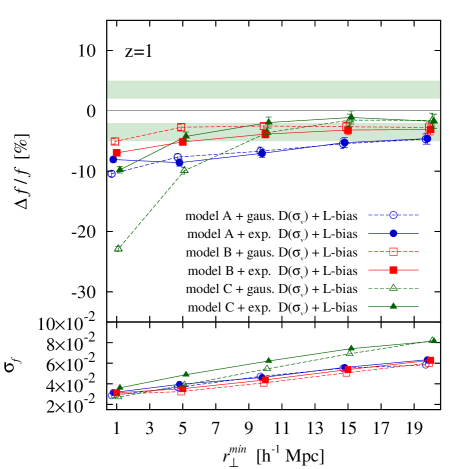
Figure 4: Top: relative systematic error on $f$ and its corresponding 1$\sigma$ uncertainty for $L>L^{*}$ galaxies at $z=1$, in the case of models for which galaxy bias is assumed to be linear. The light (dark) shaded band marks the $2\%$ ($5\%$) region around the fiducial value. Bottom: 1$\sigma$ statistical error on $f$ in the case of a survey probing $1~{}{\rm h}^{-3}~{}{\rm Gpc}^{3}$.

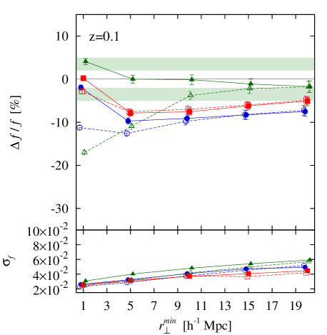
Figure 5: Same as Fig. 4 but at redshift $z=0.1$.

Let us first study the effect of using different combinations of Kaiser term and damping function with the assumption that galaxy bias is linear and scale-independent. We use the full galaxy catalogues at $z=1$ and $z=0.1$ and estimate the statistical and systematic errors on the growth rate with the different models, varying the minimum perpendicular scale used in the fit, $r_{\perp}$. In this and the following section, we consider simulated galaxies with luminosities $L>L^{*}$ (see Appendix B for details), having linear biases of $b_{L}=1.34$ and $b_{L}=2.01$ respectively at $z=0.1$ and $z=1$. These values are realistically close to current observations (e.g. Norberg et al. 2001; Pollo et al. 2005; Coil et al. 2006; Zehavi et al. 2011).

The different models behave quite similarly at both $z=1$ and $z=0.1$, as shown respectively in Fig. 4 and Fig. 5. The systematic errors on the growth rate are significant using any of the model variants, and depends on the chosen minimum scale for the fit, $r_{\perp}^{min}$. Although in general all models tend to underestimate the growth rate, the systematic errors gradually diminishes while passing from model A to model C, the latter performing best. In particular, in the case of model C with exponential damping (C-exp), $|\Delta f/f|$ always remains below $2\%$ at both redshift $z=1$ and $z=0.1$ for $r_{\perp}^{min}>10{\rm h}^{-1}~{}\rm{Mpc}$. Model B perform substantially worse, underestimating the growth rate by $3-7\%$ and $5-8\%$ at $z=1$ and $z=0.1$ respectively. Finally, we note that model A with exponential damping (A-exp) applied to scales $r_{\perp}^{min}<10{\rm h}^{-1}~{}\rm{Mpc}$, which is one of the most commonly used models in the literature, performs worst, systematically underestimating $f$ by up to $10\%$ in agreement with recent analysis (e.g. Bianchi et al. 2012).

These results are qualitatively consistent with the power spectrum analysis of Kwan et al. (2012), who show that for dark matter only at $z=0$, $z=0.5$ and $z=1$, model C with Gaussian damping (C-gauss) is the least biased model when fitting up to $k_{max}=0.1$. Our tests show however that for galaxies, model C-exp is less biased than C-gauss. In fact, the choice of damping function has only a significant impact on the model’s ability to handle small scales, with the difference diminishing with increasing $r_{\perp}^{min}$ given the similar asymptotic behaviour of the two functional forms. Conversely, we note that the Gaussian damping produces in general slightly lower statistical errors than the exponential damping. These tend also to be about $15\%$ smaller for models A and B than for model C.

It is important to note that for $r_{\perp}^{min}<10{\rm h}^{-1}~{}\rm{Mpc}$, the accuracy with which $f$ is recovered tends to deteriorate for all models. This is plausibly associated with the increase of non-linearities in galaxy clustering. In this regime, the assumption of linear biasing breaks down and it becomes crucial to account for non-linearities to recover unbiased measurements of the growth rate, as we will discuss in the next sections.

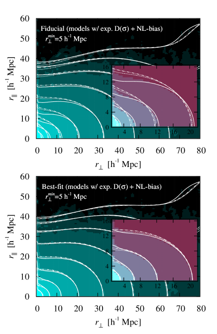
Figure 6: Measured $\xi(r_{\perp},r_{\parallel})$ and associated models for $L>L^{*}$ galaxies at $z=1$. In each panel the dotted, dot-dashed, and solid curves correspond respectively to model A, B, and C with exponential damping and linear bias, while the contours correspond to the measured $\xi(r_{\perp},r_{\parallel})$ in the galaxy catalogue. The top panel shows the fiducial prediction of the models while the bottom panel shows the best-fitting model when the parameters ($f$,$\sigma_{v}$,$b_{L}$) are allowed to vary. We note the fiducial value for $\sigma_{v}$ is fixed to its linear value. In this figure, the measured $\xi(r_{\perp},r_{\parallel})$ is smoothed using a Gaussian kernel of size $0.5{\rm h}^{-1}~{}\rm{Mpc}$.

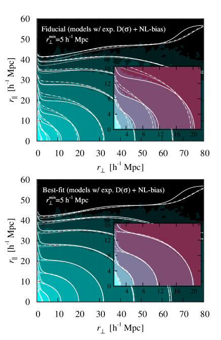
Figure 7: Same as Fig. 6 but at $z=0.1$.

3.3 Effect of galaxy scale-dependent bias

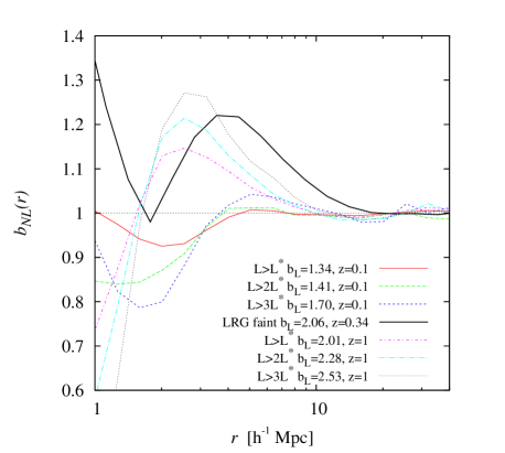
Figure 8: The scale dependence of galaxy bias at $z=0.1$ and $z=1.0$, for the different galaxy populations considered in this work (see inset). It is defined as $b_{NL}(r)=\left[\xi_{gg}(r)/\left(b^{2}_{L}\xi_{\mathrm{\delta\delta}}(r)\right)\right]^{1/2}$.

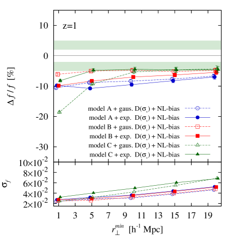
Figure 9: Top: relative systematic error on $f$ and its corresponding 1$\sigma$ uncertainty for $L>L^{*}$ galaxies at $z=1$, when the bias scale dependence is included. The light (dark) shaded band marks the $2\%$ ($5\%$) region around the fiducial value. Bottom: 1$\sigma$ statistical error on $f$ in the case of a survey probing $1~{}{\rm h}^{-3}~{}{\rm Gpc}^{3}$.

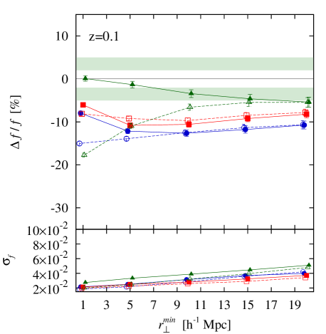
Figure 10: Same as Fig. 9 but at $z=0.1$.

We now allow for scale-dependence in the galaxy bias description inside the models and study whether this can improve the recovery of the growth rate parameter, in particular when including scales below $10{\rm h}^{-1}~{}\rm{Mpc}$ in the fitting. In general, the galaxy bias in configuration space can be defined as,

$$b(r)=\left(\frac{\xi_{gg}(r)}{\xi_{\mathrm{\delta\delta}}(r)}\right)^{1/2}=b_{L}b_{NL}(r)$$ (41)

where $\xi_{gg}$ is the galaxy real-space auto-correlation function and $b_{NL}(r)$ is the non-linear scale-dependent part of the bias. It is important to stress that $\xi_{gg}(r)$ is directly measurable from observations by deprojecting the observed projected correlation function $w(r_{\perp})$ (Saunders et al. 1992). This procedure allows one to correctly recover the shape of $\xi_{gg}(r)$ up to about $30{\rm h}^{-1}~{}\rm{Mpc}$ (e.g. Saunders et al. 1992; Cabré & Gaztañaga 2009b) while it can possibly introduce noise. In general the latter can increase the statistical error but may not introduce any systematic bias in the recovery of $f$ (Marulli et al. 2012), although this has to be investigated in more details in practical applications. In the following we will therefore make the assumption that the real-space galaxy auto-correlation function $\xi_{gg}(r)$ is known, and used its measured values from the simulated catalogues to infer $b_{NL}(r)$ in the models. In fact, it is not necessary to know the exact shape of $\xi_{gg}(r)$ on scales larger than about $20-30$$\,{\rm h}^{-1}$ Mpc, where one generally finds the galaxy bias to be almost scale-independent and can thus safely assume $b_{NL}(r)=1$. A notable exception is that of more non-linear objects, for which the scale dependence may extend to larger scales (see section 3.3.2).

Fig. 8 shows the non-linear scale-dependent component of galaxy bias, $b_{NL}(r)$, for the different galaxy populations in our simulated catalogues at the two reference redshifts considered, $z=1$ and $z=0.1$. In the previous section we considered only catalogues of galaxies with $L>L^{*}$, while in this figure we introduce more extreme galaxy populations, which we analyse in the following section. To define $b_{NL}(r)$, the linear bias $b_{L}$ has been determined for each galaxy population by minimising the difference between $\xi_{gg}$ and $b^{2}_{L}\xi_{\mathrm{\delta\delta}}$ on scales above $r=10{\rm h}^{-1}~{}\rm{Mpc}$. It is evident from this figure that non-linearities in the galaxy bias produce variations up to $40\%$ in the real-space clustering on scales $1{\rm h}^{-1}~{}\rm{Mpc}<r<20{\rm h}^{-1}~{}\rm{Mpc}$, the strength of the effect increasing for more luminous galaxies.

Let us come back to our original $L>L^{*}$ catalogues and repeat the analysis of the previous section now including the scale dependence of galaxy bias shown in Fig. 8. The new statistical and systematic errors on $f$ estimated from our simulated catalogues are shown in Figs. 9 and 10. In general, one sees that including the bias scale-dependence information has only the effect of shifting the recovered $f$ values by about $-3\%$ at both $z=1$ and $z=0.1$. This systematic effect is not straightforward to explain but could be due to degeneracies in the models when including this extra degree of freedom. Accounting for bias scale dependence tends however to reduce the dependence of the systematic error on the minimum fitted scale when including scales below $r_{\perp}=10{\rm h}^{-1}~{}\rm{Mpc}$: the retrieved value is more constant down to $r_{\perp}^{min}=1{\rm h}^{-1}~{}\rm{Mpc}$ for all considered models. Moreover, it reduces the statistical error on $f$ by about $15\%$ for all models.

These results suggest that including the bias scale-dependence empirically in the models in the way presented here, does not significantly improve the modelling of $\xi(r_{\perp},r_{\parallel})$ on scales below $10{\rm h}^{-1}~{}\rm{Mpc}$. A more detailed inclusion of galaxy bias and its non-linearities in redshift-space distortions models might be needed.

3.3.1 Fidelity in reproducing the anisotropic two-point correlation function

We visually compare in Fig. 6 and Fig. 7 the model correlation functions at $z=1$ and $z=0.1$ using (a) the fiducial values of the parameters ($f$, $\sigma_{v}$, $b_{L}$) and (b) their best-fit values obtained with the chosen model, to those measured in our simulated catalogues. For case (a), $\sigma_{v}$ is set to linear theory prediction which is given by Eq. 12, replacing $P_{\mathrm{\theta\theta}}$ by the linear power spectrum. We limit this comparison to the case with exponential damping, scale-dependent bias, and $r_{\perp}^{min}=5{\rm h}^{-1}~{}\rm{Mpc}$.

As shown in the top panels, when all parameters are fixed to their fiducial value, model C (solid line) provides a good description of the observed $\xi(r_{\perp},r_{\parallel})$ in the catalogues, with a slightly worse match for $r_{\perp}<10{\rm h}^{-1}~{}\rm{Mpc}$, $r_{\parallel}>10{\rm h}^{-1}~{}\rm{Mpc}$ particularly at $z=1$. Conversely, model A and B produce contours that at intermediate separations ($r_{\perp}<40{\rm h}^{-1}~{}\rm{Mpc}$, $r_{\parallel}<25-30{\rm h}^{-1}~{}\rm{Mpc}$) are less squashed along the line-of-sight than the data. It is important to keep in mind that our description of model B and C on scales below $r\simeq 10.5~{}{\rm h}^{-1}~{}\rm{Mpc}$ may be biased as we lack information on the small-scale amplitude of $\xi_{\mathrm{\delta\theta}}(r)$ and $\xi_{\mathrm{\theta\theta}}(r)$ in their construction (see Section 2.4). When ($f$, $\sigma_{v}$, $b_{L}$) are allowed to vary (lower panels), all models are generally capable to achieve a good fit to $\xi(r_{\perp},r_{\parallel})$ above $r_{\perp}=10{\rm h}^{-1}~{}\rm{Mpc}$. For model A and B, this is obtained through a lower damping than predicted by linear theory. This allows one to reproduce the significant squashing along the line-of-sight seen in the catalogues, but fails to model the FoG elongation at smaller $r_{\perp}$.

In general, low values of $\sigma_{v}$ can balance the deficit of power on small scales, yet they do not allow to recover the true value of $f$. This is shown in Fig. 11 and 12, where the recovered values of $\sigma_{v}$ for the different models are compared to linear prediction. While model C is able to recover realistic values of $\sigma_{v}$, of the order of linear theory predictions, model A and B provides best-fitting values strongly deviating from linear expectations, leading to $\sigma_{v}$ as small as $0-200\,{\rm km\cdot s^{-1}}$. These results are consistent with the findings of Taruya et al. (2010) and Nishimichi & Taruya (2011), who compared model A and C in the case of dark matter and halo catalogues, finding a better agreement of the recovered $\sigma_{v}$ with linear theory in the case of model C. These findings confirm that model C is probably less degenerate than A and B regarding its description of streaming and random velocities.

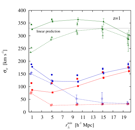
Figure 11: Recovered values of $\sigma_{v}$ for the different models in the case of $L>L^{*}$ galaxies at $z=1$. The symbol definition is the same as in Fig. 4. The connected points correspond to the case with scale-dependent bias, while others correspond to that with linear bias. The latter points are slightly shifted horizontally for clarity.

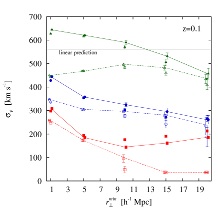
Figure 12: Same as Fig. 11 but at $z=0.1$.

3.3.2 The case of highly-biased galaxies

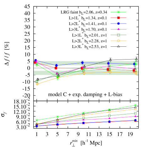
Figure 13: Top: relative systematic error on $f$ and its corresponding 1$\sigma$ uncertainty for different galaxy populations at various redshifts (see inset). In all cases we use model C-exp with linear bias. The light (dark) shaded band marks the $2\%$ ($5\%$) region around the fiducial value. Bottom: 1$\sigma$ statistical error on $f$ in the case of a survey probing $1~{}{\rm h}^{-3}~{}{\rm Gpc}^{3}$, except in the case of the LRG sample where the quoted value is for a survey of $13.8~{}{\rm h}^{-3}~{}{\rm Gpc}^{3}$ (see text for details).

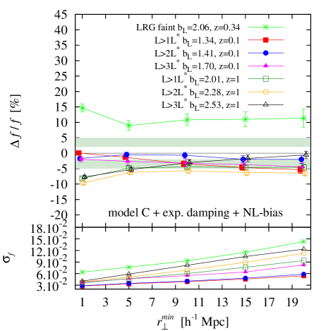
Figure 14: Same as Fig. 13 but in the case where the bias is scale-dependent.

Highly biased objects are in general favoured tracers by redshift-space distortions studies by virtue of the fact that they probe larger volumes of the Universe. However, these objects, which are more likely to reside in the most massive haloes, have undergone a stronger non-linear evolution, this explaining their stronger bias scale-dependence seen in Fig. 8. As such, the inclusion of $b_{NL}$ in the models may become even more critical for these objects, if one’s goal is to accurately measure the growth rate parameter (e.g. Cabré & Gaztañaga 2009a). In this section, we explicitly test this hypothesis, extending the model comparison to the regime of highly biased galaxy populations.

Let us first define higher-luminosity galaxies from our simulated catalogues. We shall consider two sub-samples, defined as including galaxies with $L>2L^{*}$ and $L>3L^{*}$. We complement these with a catalogue of simulated Luminous Red Galaxies (LRG) drawn from the “LasDamas” suite of simulations, meant to accurately reproduce the galaxy clustering in the SDSS-DR7 release (McBride et al., in preparation). More precisely, we shall use 100 mock realisations of what are defined as “faint LRG” ($M_{r}<-21.2$). These mock samples, which are in fact lightcones, have been constructed by populating haloes with galaxies in 40 cubic dark matter N-body simulations of $2400{\rm h}^{-1}~{}\rm{Mpc}$ a side and resolution $m_{p}=45.73\times 10^{10}~{}\rm{h^{-1}}~{}\rm{M_{\odot}}$. When fitting the measured $\xi(r_{\perp},r_{\parallel})$ in those catalogues, we use in the models the non-linear mass power spectrum given by CAMB for the cosmological parameters of the LasDamas simulations. This includes non-linear evolution of clustering as described by Smith et al. (2003).

We compare in Fig. 13 and Fig. 14 the relative systematic error on the growth rate obtained for these highly biased galaxies. We use here model C-exp with and without including the scale-dependence of bias. In the case of the linearly-biased model, the systematic error on the growth rate remains within $\pm 5\%$ at $r_{\perp}^{min}>10{\rm h}^{-1}~{}\rm{Mpc}$, for all considered galaxy populations, but those with $L>3L^{*}$ at $z=1$, which are the most biased objects considered in this analysis. In the latter case the growth rate is overestimated by about $6-7\%$, suggesting additional non-linear effects that are not accounted for in our models.

When including scale-dependent bias, for all but LRG, the dispersion among the recovered growth rates is reduced and systematic errors remain within $-7\%<\Delta f/f<-2\%$ when $r_{\perp}^{min}>5{\rm h}^{-1}~{}\rm{Mpc}$. In the case of LRG, the growth rate is overestimated by about $10\%$ and the associated statistical error is higher. It is important to mention that LRG statistical errors on $f$ in the figures correspond to a cosmological volume larger by $2.4^{3}$ than for the other samples. Thus, in order to make a fair comparison, one has to further multiply the quoted LRG statistical errors by the square root of the ratio between the volumes (e.g. Bianchi et al. 2012), i.e. by about $3.7$. A cautionary remark in interpreting this result is that the simulated LRG samples are, unlike the other samples considered, relatively wide lightcones and as a consequence, may include wide-angle effects that are not accounted for in our models (but see Samushia et al. 2011a).Moreover, although this sample has been already used for other investigations, we have no way to verify the details of the HOD implementation and its impact on our results.

Overall these results confirm our previous findings, suggesting that for highly non-linearly biased galaxies, additional systematic effects arise which could be due to an incorrect inclusion of scale-dependence of bias into the model. From a theoretical point-of-view, bias non-linearity changes the correction terms $C_{A}$ and $C_{B}$ in model C, which might need to be modified to properly include galaxy bias non-linearities and scale-dependence (see Tang et al. 2011; Nishimichi & Taruya 2011). We plan to investigate in more details these aspects in a future paper. Finally, we note that FoG modelling could be potentially improved by adding more freedom in the damping function (e.g. Kwan et al. 2012) or including scale dependence in the pairwise velocity dispersion (e.g. Hawkins et al. 2003), but at the price of increasing the statistical error on the growth rate estimate.

4 Effect of galaxy velocity bias

In the framework of understanding the impact of non-linear effects on the accuracy of growth rate estimates from redshift-space distortions, we investigate in this section the possible impact of velocity bias, an effect which is is usually neglected. The galaxy catalogues that we used so far, assume that the radial distribution of satellite galaxies inside dark-matter halos follows that of mass, as described by a Navarro et al. (1996) (NFW) radial density profile. Moreover, central galaxies have been defined as being at rest at the centre of their dark matter halo, inheriting its mean velocity. These assumptions make galaxy velocities unbiased with respect to the mass velocity field. However, there are some observational evidences that galaxies does not exactly follow the same radial distribution as dark matter and exhibit some velocity bias. In particular, recent small-scale clustering measurements in the SDSS suggest that relatively luminous galaxies have a steeper radial density profile than NFW, with inner slopes close to $-2$ and lower concentration parameters (Watson et al. 2012). In addition, galaxy groups and galaxy clusters analysis tend to indicate that central galaxies might in general not be exactly at rest at the centre of the potential well of dark matter haloes (e.g. van den Bosch et al. 2005; Skibba et al. 2011). Differences between the radial distribution of galaxies and that of mass implies the presence of additional spatial and velocity biases. This has a direct impact on the description of the observed redshift-space distortions. In this section we provide a first quantitative assessment of the systematic uncertainty on $f$ that it can introduce if not accounted for in the models.

To this end, we include in the catalogues some amount of velocity bias coming from either central or satellite galaxies. For central galaxies we follow van den Bosch et al. (2005) and assign halo-centric positions assuming a radial density distribution of the form,

$$\rho_{cen}(r|m)\propto\frac{\displaystyle f_{r}r_{v}(m)}{\displaystyle r\left(r+f_{r}r_{v}(m)\right)^{3}}$$ (42)

where $m$ is the halo mass, $r_{v}$ is the halo virial radius, and $f_{r}$ is a free parameter that controls the amount of spatial and velocity bias introduced. This effectively offsets central galaxies from their halo centre of mass. By solving Jeans equation one obtains the associated one-dimensional velocity dispersion,

$$\sigma^{2}_{cen}(r|m)=\frac{1}{\rho_{cen}(r|m)}\int_{r}^{\infty}\rho_{cen}(r|m)\frac{d\psi}{dr}dr$$ (43)

where $\psi(r)$ is gravitational potential. One can thus define the velocity bias of central galaxies as,

$$b^{cen}_{v}(m)=\frac{\left<\sigma_{cen}|m\right>}{\left<\sigma_{dm}|m\right>},$$ (44)

where the halo-averaged velocity dispersions are given by,

$$\left<\sigma_{cen}|m\right> ={}\frac{4\pi}{m}\displaystyle\int_{0}^{r_{v}(m)}\rho_{cen}(r|m)\sigma_{cen}(r|m)r^{2}dr$$ (45)

$$\left<\sigma_{dm}|m\right> ={}\frac{4\pi}{m}\displaystyle\int_{0}^{r_{v}(m)}\rho_{NFW}(r|m)\sigma_{NFW}(r|m)r^{2}dr$$ (46)

and the NFW radial density profile is defined as,

$$\rho_{NFW}(r|m)\propto\left(\frac{c_{dm}(m)r}{r_{v}(m)}\right)^{-1}\left(1+\frac{c_{dm}(m)r}{r_{v}(m)}\right)^{-2}$$ (47)

where $c_{dm}$ is the dark matter concentration parameter (see Appendix B for its definition). Galaxy halo-centric velocities are drawn from a Gaussian distribution in each dimension with velocity dispersion given by Eq. 43. We choose the value of $f_{r}$ in order to have $b^{cen}_{v}(m)=0.2$. The latter is an average value motivated by recent observations (e.g. Coziol et al. 2009; Skibba et al. 2011).

In the case of satellite galaxies we followed a similar methodology. Based on the recent results of Watson et al. (2012) in the SDSS for $M_{r}<-20.5$ galaxies, we radially distribute satellite galaxies as to reproduce a generalised radial density profile of the form,

$$\rho_{sat}(r|m)\propto\left(\frac{c_{sat}(m)r}{r_{v}(m)}\right)^{-\gamma}\left(1+\frac{c_{sat}(m)r}{r_{v}(m)}\right)^{-3+\gamma}$$ (48)

with $c_{sat}(m)=\frac{c_{dm}(m)}{2}$ and $\gamma=2$. As for central galaxies, we assign satellite galaxy velocities from the associated one-dimensional velocity dispersion,

$$\sigma^{2}_{sat}(r|m)=\frac{1}{\rho_{sat}(r|m)}\int_{r}^{\infty}\rho_{sat}(r|m)\frac{d\psi}{dr}dr.$$ (49)

This leads to a velocity bias,

$$b^{sat}_{v}(m)=\frac{\left<\sigma_{sat}|m\right>}{\left<\sigma_{dm}|m\right>},$$ (50)

where

$$\left<\sigma_{sat}|m\right>=\frac{4\pi}{m}\displaystyle\int_{0}^{r_{v}(m)}\rho_{sat}(r|m)\sigma_{sat}(r|m)r^{2}dr.$$ (51)

In that case, $b^{sat}_{v}(m)$ slowly increases from $b^{sat}_{v}=1$ at $m=10^{9}~{}h^{-1}~{}M_{\odot}$ to $b^{sat}_{v}\simeq 1.2$ at $m=10^{16}~{}h^{-1}~{}M_{\odot}$. Assuming that the haloes are spherical and isotropic, all previous integrals can be solved analytically (see e.g. Appendix B and van den Bosch et al. 2005).

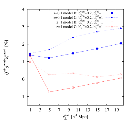
Figure 15: Percent systematic variation of the measured growth rate $(f^{vb}-f^{novb})/f^{novb}$ induced by including some amount of velocity bias from central galaxies in the simulated catalogues. Galaxies with $L>L^{*}$ at the two reference redshifts are considered, applying models B-exp and C-exp with scale-dependent bias.

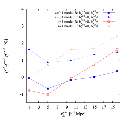
Figure 16: Same as Fig. 15 but when including velocity bias coming from satellite galaxies in the simulated catalogues.

Fig. 15 and 16 show the percent variation on the estimated $f$, when a velocity bias is included in the simulated catalogues according to the previously described procedure. The curves show the systematic effect of velocity bias coming from either central or satellite galaxies, when $f$ is estimated from models B-exp and C-exp assuming a scale-dependent spatial bias. We find that the impact of central galaxy velocity bias is smaller than that of satellite galaxies: at $z=0.1$ a velocity bias of $b_{v}^{cen}=0.2$ introduces a negative systematic error of about $1\%$, independently of the model. At $z=1$ the effect is larger, with a systematic error that can reach about $-3\%$ over the range $1{\rm h}^{-1}~{}\rm{Mpc}<r_{\perp}^{min}<20{\rm h}^{-1}~{}\rm{Mpc}$. We should note that the test at $z=1$ may be pessimistic, as the amount of velocity bias introduced in the catalogues corresponds to observational constraints from the local Universe and it is plausible that at $z=1$ the actual velocity bias is lower. In the case of satellite galaxies, the introduction of a velocity bias has a stronger impact: at $z=1$ the systematic error remains within $1-2\%$, while at $z=0.1$ it is of about $2-3\%$, depending on the model used. In the latter case, we note that model C tend to be less affected.

These admittedly simple tests suggest that velocity bias, if not accounted for in the models, can introduce additional systematic errors of the order of $1-3\%$, i.e. of the same order of statistical errors expected to be reachable by future large surveys. Although not dramatic, this additional source of systematic error needs to be kept in mind and possibly accounted for in future models. In principle, galaxy velocity bias can be included in the models by adding an effective velocity bias factor in front of the terms involving the velocity divergence field. At first approximation, one could assume this velocity bias factor to be constant and set it as a free parameter while fitting redshift-space distortions. Introducing more degrees of freedom in the models would however inevitably increase statistical errors.

5 Summary and conclusions

Measurements of the growth rate of structure from redshift-space distortions have come to be considered as one of the most promising probes for future massive redshift surveys that aim at solving the dilemma of cosmic acceleration. A notable example is the survey planned for the approved ESA Euclid space mission (Laureijs et al. 2011). In this paper, we have investigated in some detail how well non-linear effects can be accounted for by current models when performing such measurements on galaxy catalogues. The question is how to optimally use observations and models, in order to minimise statistical and systematic errors alike. The actual extraction of the redshift-space distortions signal from real data is subject to two competing requirements. On one hand, one would like to use the simple linear description of redshift-space distortions induced by large-scale coherent motions, thus limiting the measurements and modelling to very large scales. On such scales fluctuations are close to be linear and systematic effects appear to be reduced (e.g. Samushia et al. 2011a). On the other hand, the clustering signal on those scales is so weak that statistical errors on the measured growth rate remain large, even when using samples probing large volumes. One may therefore prefer to extend the modelling to smaller scales, enlarging the range of analysed scales and thus reducing the statistical error.

The most effective compromise to exploit the size and statistics of future surveys seems thereby that of including intermediate quasi-nonlinear scales, at the expense of a more complicated modelling effort. As discussed in the introduction, most recent developments in this direction have so far concentrated on improving the description of non-linear effects in the redshift-space clustering of matter fluctuations in Fourier space. Here we have investigated how these models perform when applied to catalogues of realistic galaxies in configuration space, in both the local Universe at $z=0.1$ and the more distant Universe at $z=1$. For this purpose, we have reformulated in terms of the anisotropic two-point correlation function of galaxies $\xi(r_{\perp},r_{\parallel})$, the analytical model for the redshift-space anisotropic power spectrum by Scoccimarro (2004) as well as the recent improvements proposed by Taruya et al. (2010), in addition to the standard dispersion model. In these models, we have included the possibility of using a realistic non-linear scale-dependent galaxy bias, the latter being in principle measurable from the observations. At variance with the usual habit of fitting for the distortion parameter $\beta=f/b_{L}$, we have considered the possibility of including the linear component of galaxy bias as a free parameter and directly estimate the growth rate of structure $f$. Our key findings and results can be summarised as follows:

1. When applied to the galaxy anisotropic correlation function, Taruya et al. (2010)’s model, the most sophisticated model considered in this analysis, generally provide the most unbiased estimates of the growth rate of structure $f$, retrieving it at the level of about $\pm 4\%$ at $z=0.1$ and $z=1$. The commonly used Scoccimarro (2004) and dispersion models generally underestimate the growth rate by $4-7\%$ and $5-10\%$ respectively.

2. The inclusion of the scale-dependence of bias in the models is important for minimising the systematic error on $f$, in particular when one uses the scales below about $10{\rm h}^{-1}~{}\rm{Mpc}$.

3. Systematic errors vary with the degree of non-linearity in the bias of the considered galaxy population, which in turn is a function of redshift. Accounting for it is therefore particularly relevant when “slicing” deep surveys to measure $f(z)$ over a significant redshift range.

4. Galaxy velocity bias could represent, if not accounted for, an additional source of systematic error. By implementing realistic prescriptions for galaxy velocity bias coming from either central or satellite galaxies in our simulated samples, we estimate that neglecting it yields to an underestimate of the recovered $f$ by $1-3\%$.

Overall, these results further emphasise the need for careful modelling of non-linear effects, if redshift-space distortions have to be used as a precision cosmology probe. Further investigation is needed on the proper inclusion of bias non-linearities, in particular when using galaxy populations with strong bias scale-dependence. This is still a non-negligible source a systematic error that has to be accounted for, to reach the percent accuracy on the growth rate. Our results nevertheless indicate promising venues along which to develop further methods to overcome systematic biases and support the hope that redshift-space distortions in future surveys will provide us with a unique test of the cosmological model.

Appendix A Redshift-space anisotropic two-point correlation function for the Taruya, Nishimichi & Saito (2010) model

The redshift-space anisotropic two-point correlation function is obtainable by Fourier-transforming the anisotropic redshift-space power spectrum $P^{s}(k,\mu)$ as,

$$\xi(r_{\perp},r_{\parallel})=\int\frac{d^{3}\mn@boldsymbol{k}}{(2\pi)^{3}}e^{i\mn@boldsymbol{k}\cdot\mn@boldsymbol{s}}P^{s}(k,\mu)=\sum_{l}\xi^{s}_{l}(s)L_{l}(\nu)$$ (52)

where $\nu=r_{\parallel}/s$, $r_{\perp}=\sqrt{s^{2}-r_{\parallel}^{2}}$, and $L_{l}$ denote Legendre polynomials. The correlation function multipole moments $\xi^{s}_{l}(s)$ are defined as,

$$\xi^{s}_{l}(s)=i^{l}\int\frac{dk}{2\pi^{2}}k^{2}P^{s}_{l}(k)j_{l}(ks),$$ (53)

where $j_{l}$ denotes the spherical Bessel functions and

$$P^{s}_{l}(k)=\frac{2l+1}{2}\int_{-1}^{1}d\mu P^{s}(k,\mu)L_{l}(\mu).$$ (54)

In the case of biased tracers of mass, Taruya et al. (2010) model for the redshift-space anisotropic power spectrum can be written as,

$$P^{s}(k,\mu) ={}D(k\mu\sigma_{v})\left[b^{2}P_{\mathrm{\delta\delta}}(k)+2b\mu^{2}fP_{\mathrm{\delta\theta}}(k)\right.$$

$$\left.+\mu^{4}f^{2}P_{\mathrm{\theta\theta}}(k)+C_{A}(k,\mu;f,b)+C_{B}(k,\mu;f,b)\right]$$ (55)

where $b$ is the spatial bias of the considered tracers and,

$$C_{A}(k,\mu;f,b) ={}\sum_{m,n=1}^{3}b^{3-n}f^{n}\mu^{2m}P_{Amn}(k),$$

$$C_{B}(k,\mu;f,b) ={}\sum_{n=1}^{4}\sum_{a,b=1}^{2}b^{4-a-b}(-f)^{a+b}\mu^{2n}P_{Bnab}(k),$$

with,

$$P_{Amn}(k) ={}\frac{k^{3}}{(2\pi)^{2}}\left[\int_{0}^{\infty}dr\int_{-1}^{+1}dx\left(A_{mn}(r,x)P(k)\right.\right.$$

$$\left.+\widetilde{A}_{mn}(r,x)P(kr)\right)\times\frac{P\left(k\sqrt{1+r^{2}-2rx}\right)}{(1+r^{2}-2rx)^{2}}$$

$$\left.+P(k)\int_{0}^{\infty}dra_{mn}(r)P(kr)\right],$$ (56)

$$P_{Bnab}(k) ={}\frac{k^{3}}{(2\pi)^{2}}\int_{0}^{\infty}dr\int_{-1}^{+1}dxB^{n}_{ab}(r,x)$$

$$\frac{P_{a2}\left(k\sqrt{1+r^{2}-2rx}\right)P_{b2}(kr)}{(1+r^{2}-2rx)^{a}},$$ (57)

where functions $A_{mn}(r,x)$, $\widetilde{A}_{mn}(r,x)$, $a_{mn}(r,x)$, $B_{ab}(r,x)$ are given in Appendix A of Taruya et al. (2010), $P(k)$ is the linear mass power spectrum, $P_{12}(k)=P_{\mathrm{\delta\theta}}(k)$, and $P_{22}(k)=P_{\mathrm{\theta\theta}}(k)$. By using the Kaiser term in Eq. 55 (i.e. Eq. 55 without the damping function $D(k\mu\sigma_{v})$) into Eq. 54 and 53, one obtains the corresponding correlation function multipole moments. The non-null multipole moments are then given by,

$$\xi^{s}_{0}(s){} =b^{2}\xi_{\mathrm{\delta\delta}}+bf\frac{2}{3}\xi_{\mathrm{\delta\theta}}+f^{2}\frac{1}{5}\xi_{\mathrm{\theta\theta}}$$

$$+b^{2}f\frac{1}{3}\xi_{A11}+bf^{2}\frac{1}{3}\xi_{A12}+bf^{2}\frac{1}{5}\xi_{A22}+f^{3}\frac{1}{5}\xi_{A23}$$

$$+f^{3}\frac{1}{7}\xi_{A33}+b^{2}f^{2}\frac{1}{3}\xi_{B111}-bf^{3}\frac{1}{3}\left(\xi_{B112}+\xi_{B121}\right)$$

$$+f^{4}\frac{1}{3}\xi_{B122}+b^{2}f^{2}\frac{1}{5}\xi_{B211}-bf^{3}\frac{1}{5}\left(\xi_{B212}+\xi_{B221}\right)$$

$$+f^{4}\frac{1}{5}\xi_{B222}-bf^{3}\frac{1}{7}\left(\xi_{B312}+\xi_{B321}\right)+f^{4}\frac{1}{7}\xi_{B322}$$

$$+f^{4}\frac{1}{9}\xi_{B422},$$ (58)

$$\xi^{s}_{2}(s){} =bf\frac{4}{3}\xi^{(2)}_{\delta\theta}+f^{2}\frac{4}{7}\xi^{(2)}_{\theta\theta}$$

$$+b^{2}f\frac{2}{3}\xi^{(2)}_{A11}+bf^{2}\frac{2}{3}\xi^{(2)}_{A12}+bf^{2}\frac{4}{7}\xi^{(2)}_{A22}+f^{3}\frac{4}{7}\xi^{(2)}_{A23}$$

$$+f^{3}\frac{10}{21}\xi^{(2)}_{A33}+b^{2}f^{2}\frac{2}{3}\xi^{(2)}_{B111}-bf^{3}\frac{2}{3}\left(\xi^{(2)}_{B112}+\xi^{(2)}_{B121}\right)$$

$$+f^{4}\frac{2}{3}\xi^{(2)}_{B122}+b^{2}f^{2}\frac{4}{7}\xi^{(2)}_{B211}-bf^{3}\frac{4}{7}\left(\xi^{(2)}_{B212}+\xi^{(2)}_{B221}\right)$$

$$+f^{4}\frac{4}{7}\xi^{(2)}_{B222}-bf^{3}\frac{10}{21}\left(\xi^{(2)}_{B312}+\xi^{(2)}_{B321}\right)+f^{4}\frac{10}{21}\xi^{(2)}_{B322}$$

$$+f^{4}\frac{40}{99}\xi^{(2)}_{B422},$$ (59)

$$\xi^{s}_{4}(s){} =f^{2}\frac{8}{35}\xi^{(4)}_{\theta\theta}$$

$$+bf^{2}\frac{8}{35}\xi^{(4)}_{A22}+f^{3}\frac{8}{35}\xi^{(4)}_{A23}+f^{3}\frac{24}{77}\xi^{(4)}_{A33}+b^{2}f^{2}\frac{8}{35}\xi^{(4)}_{B211}$$

$$-bf^{3}\frac{8}{35}\left(\xi^{(4)}_{B212}+\xi^{(4)}_{B221}\right)+f^{4}\frac{8}{35}\xi^{(4)}_{B222}-bf^{3}\frac{24}{77}\left(\xi^{(4)}_{B312}\right.$$

$$+\left.\xi^{(4)}_{B321}\right)+f^{4}\frac{24}{77}\xi^{(4)}_{B322}+f^{4}\frac{48}{143}\xi^{(4)}_{B422},$$ (60)

$$\xi^{s}_{6}(s){} =f^{3}\frac{16}{231}\xi^{(6)}_{A33}-bf^{3}\frac{16}{231}\left(\xi^{(6)}_{B312}+\xi^{(6)}_{B321}\right)+f^{4}\frac{16}{231}\xi^{(6)}_{B322}$$

$$+f^{4}\frac{64}{495}\xi^{(6)}_{B422},$$ (61)

$$\xi^{s}_{8}(s){} =f^{4}\frac{128}{6435}\xi^{(8)}_{B422},$$ (62)

where $\xi_{Amn}$ and $\xi_{Bnab}$ are the Fourier conjugate pairs of $P_{Amn}$ and $P_{Bnab}$ in Eqs. 56 and 57, and $\xi^{(l)}_{X}$ are the correlation function multipole moments associated with $P_{X}$ as defined in Eq. 53. For orders $l=2$, $l=4$, $l=6$ and $l=8$, the latter can be conveniently rewritten as,

$$\xi^{(2)}_{X}(r) ={}\xi_{X}(r)-3X_{2}(r)$$ (63)

$$\xi^{(4)}_{X}(r) ={}\xi_{X}(r)+\frac{15}{2}X_{2}(r)-\frac{35}{2}X_{4}(r)$$ (64)

$$\xi^{(6)}_{X}(r) ={}\xi_{X}(r)-\frac{105}{8}X_{2}(r)+\frac{315}{4}X_{4}(r)$$

$$+\frac{693}{8}X_{6}(r)$$ (65)

$$\xi^{(8)}_{X}(r) ={}\xi_{X}(r)+\frac{315}{16}X_{2}(r)-\frac{3465}{16}X_{4}(r)$$

$$-\frac{9009}{16}X_{6}+\frac{6435}{16}X_{8}(r)$$ (66)

where,

$$X_{n}(r)=r^{-(n+1)}\int_{0}^{r}\xi_{X}(r^{\prime})r^{\prime n}dr^{\prime}.$$ (67)

These identities, which orders $l=2$ and $l=4$ were already found by Hamilton (1992) and Cole et al. (1994), are obtained by using recurrence relations and integral forms of spherical Bessel functions (see Toyoda & Ozaki 2010, for details).

Although the model predicts non-null multipole moments of orders $l=6$ and $l=8$, we neglected these terms in this analysis, including only correlation function multipole moments $\xi^{s}_{0}(s)$, $\xi^{s}_{2}(s)$, and $\xi^{s}_{4}(s)$ (see main text).

Appendix B HOD galaxy catalogue construction

We describe in this appendix the method that we used to create realistic galaxy catalogues from a large N-body dark matter simulation, based on the Halo Occupation Distribution (HOD) formalism (e.g. Cooray & Sheth 2002).

We used the dark matter haloes identified using a friends-of-friends algorithm with linking length of $l=0.17$ in the MDR1 dark matter simulation by Prada et al. (2011). Halo masses were estimated from the sum of dark matter particle masses inside each halo after correcting for finite force and mass resolution (Bhattacharya et al. 2011, Eq. 4). We populated haloes according to their mass by specifying the galaxy halo occupation which we parametrise as,

$$\left<N_{gal}|m\right>=\left<N_{cen}|m\right>(1+\left<N_{sat}|m\right>)$$ (68)

where $\left<N_{cen}|m\right>$ and $\left<N_{sat}|m\right>$ are the average number of central and satellite galaxies in a halo of mass $m$. Central and satellite galaxy occupations are defined as (Zheng et al. 2005),

$$\left<N_{cen}|m\right> = \frac{1}{2}\left[1+\rm{erf}\left(\frac{\log~{}m-\log M_{min}}{\sigma_{\log~{}m}}\right)\right],$$ (69)

$$\left<N_{sat}|m\right> = \left(\frac{m-M_{0}}{M_{1}}\right)^{\alpha}.$$ (70)

where $M_{min}$, $\sigma_{\log~{}m}$, $M_{0}$, $M_{1}$, and $\alpha$ are HOD parameters.

We positioned central galaxies at halo centres with probability given by a Bernoulli distribution function with mean taken from Eq. 69 and assigned host halo mean velocities to them. The number of satellite galaxies per halo is set to follow a Poisson distribution with mean given by Eq. 70. We assumed that satellite galaxies follow the spatial and velocity distribution of mass and randomly distributed their halo-centric radial position as to reproduce a Navarro et al. (1996) (NFW) radial profile,

$$\rho_{NFW}(r|m)\propto\left(\frac{c_{dm}(m)r}{r_{v}(m)}\right)^{-1}\left(1+\frac{c_{dm}(m)r}{r_{v}(m)}\right)^{-2}$$ (71)

where $c_{dm}$ is the concentration parameter and $r_{v}(m)$ is the virial radius defined as,

$$r_{v}(m)=\left(\frac{3m}{4\pi\bar{\rho}(z)\Delta_{NL}}\right)^{1/3}.$$ (72)

In this equation, $\bar{\rho}(z)$ is the mean matter density at redshift $z$ and $\Delta_{NL}=200$ is the critical overdensity for virialisation in our definition. Consistently with the works of Zehavi et al. (2011), Zheng et al. (2007), and Coupon et al. (2012) that we used to infer the mean galaxy occupation, we assumed the mass-concentration relation of Bullock et al. (2001),

$$c_{dm}(m,z)=\frac{c_{0}}{1+z}\left(\frac{m}{m_{*}}\right)^{\beta}$$ (73)

where $c_{0}=11$, $\beta=-0.13$, and $m_{*}$ is the non-linear mass scale at $z=0$ defined such as $\sigma(m_{*},0)=\delta_{c}$. Here $\delta_{c}$ and $\sigma(m,0)$ are respectively the critical overdensity (we fixed $\delta_{c}=1.686$) and the standard deviation of mass fluctuations at $z=0$. The latter is defined as,

$$\sigma^{2}(m,z)=\int_{0}^{\infty}\frac{dk}{k}\frac{k^{3}P(k,z)}{2\pi^{2}}|W(kR)|^{2}\,\,\,\,.$$ (74)

where $R=\left[3m/\left(4\pi\bar{\rho}(z)\right)\right]^{1/3}$, $P(k,z)$ is the linear mass power spectrum at redshift $z$ in the adopted cosmology, and $W(x)$ is the Fourier transform of a top-hat filter.

In order to assign satellite galaxy velocities, we assumed halo isotropy and sphericity, and drawn velocities from Gaussian distribution functions along each Cartesian dimension with velocity dispersion given by (van den Bosch et al. 2004),

$$\sigma^{2}_{sat}(r|m) ={}\frac{1}{\rho_{NFW}(r|m)}\int_{r}^{\infty}\rho_{NFW}(r|m)\frac{d\psi}{dr}dr$$ (75)

$$={}\frac{Gm}{r_{v}}\frac{c_{dm}}{f(c_{dm})}\left(\frac{c_{dm}r}{r_{v}}\right)\left(1+\frac{c_{dm}r}{r_{v}}\right)^{2}I(r/rs)$$ (76)

where $\psi(r)$ is the gravitational potential, $G$ is the gravitational constant, $f(x)=\ln(1+x)-x/(1+x)$, and

$$I(x)=\int_{x}^{\infty}\frac{f(t)dt}{t^{3}(1+t)^{2}}.$$ (77)

Table 1: HOD parameters and associated galaxy catalogue properties.

Redshift	Luminosity	Absolute magnitude						Galaxy number
$z$	threshold	threshold	$\log M_{min}$	$\sigma_{\log~{}m}$	$\log M_{0}$	$\log M_{1}$	$\alpha$	density
$0.1$	$L>L^{*}$	$M_{r}-5\log(h)<-20.44$	12.18	0.21	12.18	13.31	1.08	0.347
$0.1$	$L>2L^{*}$	$M_{r}-5\log(h)<-21.19$	12.89	0.68	12.89	13.89	1.17	0.105
$0.1$	$L>3L^{*}$	$M_{r}-5\log(h)<-21.63$	13.48	0.70	13.48	14.35	1.23	0.026
$1$	$L>L^{*}$	$M_{B/g^{\prime}}-5\log(h)<-20.78$	12.29	0.35	12.29	13.36	1.23	0.200
$1$	$L>2L^{*}$	$M_{B/g^{\prime}}-5\log(h)<-21.53$	12.67	0.38	12.67	13.77	1.42	0.072
$1$	$L>3L^{*}$	$M_{B/g^{\prime}}-5\log(h)<-21.97$	12.94	0.40	12.94	14.10	1.54	0.032

Masses are given in $\rm{h^{-1}}~{}\rm{M_{\odot}}$ and galaxy number densities in $10^{-2}~{}\rm{h^{3}}~{}\rm{Mpc^{-3}}$.

We generated catalogues corresponding to different populations of galaxies defined such that their luminosity is greater than multiples of the characteristic luminosity at both $z=0.1$ and $z=1$. For this purpose, we used the HOD parameters obtained from the SDSS survey at $z\simeq 0.1$ by Zehavi et al. (2011) and interpolated the parameter dependence on luminosity threshold to build catalogues for $L>L^{*}$, $L>2L^{*}$, and $L>3L^{*}$ galaxies. For $z=1$ catalogues, we used the HOD parameters measured by Coupon et al. (2012) and Zheng et al. (2007) respectively in the CFHTLS and DEEP2 surveys. In that case, while the two analysis use slightly different selection magnitude bands ($g^{\prime}$ and $B$), we assumed here that the later give comparable luminosities (the two bands largely overlap in wavelength) and interpolate between the parameters indifferently of the band. The parameter $M_{0}$ is poorly constrained by current observations and we decided to fix $M_{0}=M_{min}$. We found that this approximation does not introduce any significant effect on the halo occupation and predicted clustering. The characteristic absolute magnitudes at $z=0.1$ and $z=1$ that we used to define the galaxy samples were taken from Blanton et al. (2003) and Ilbert et al. (2005) respectively. The catalogue properties and HOD parameters are summarised in Table LABEL:tab.

References

- Albrecht et al. (2006) Albrecht, A., Bernstein, G., Cahn, R., et al. 2006, ArXiv Astrophysics e-prints
- Anderson et al. (2012) Anderson, L., Aubourg, E., Bailey, S., et al. 2012, ArXiv e-prints
- Bhattacharya et al. (2011) Bhattacharya, S., Heitmann, K., White, M., et al. 2011, ApJ, 732, 122
- Bianchi et al. (2012) Bianchi, D., Guzzo, L., Branchini, E., et al. 2012, ArXiv e-prints
- Blake et al. (2011a) Blake, C., Brough, S., Colless, M., et al. 2011a, MNRAS, 415, 2876
- Blake et al. (2011b) Blake, C., Davis, T., Poole, G. B., et al. 2011b, MNRAS, 415, 2892
- Blanton et al. (2003) Blanton, M. R., Hogg, D. W., Bahcall, N. A., et al. 2003, ApJ, 592, 819
- Bullock et al. (2001) Bullock, J. S., Kolatt, T. S., Sigad, Y., et al. 2001, MNRAS, 321, 559
- Cabré & Gaztañaga (2009a) Cabré, A. & Gaztañaga, E. 2009a, MNRAS, 393, 1183
- Cabré & Gaztañaga (2009b) Cabré, A. & Gaztañaga, E. 2009b, MNRAS, 396, 1119
- Cai & Bernstein (2012) Cai, Y.-C. & Bernstein, G. 2012, MNRAS, 2647
- Carlson et al. (2009) Carlson, J., White, M., & Padmanabhan, N. 2009, Phys. Rev. D, 80, 043531
- Carroll et al. (2004) Carroll, S. M., Duvvuri, V., Trodden, M., & Turner, M. S. 2004, Phys. Rev. D, 70, 043528
- Coil et al. (2006) Coil, A. L., Newman, J. A., Cooper, M. C., et al. 2006, ApJ, 644, 671
- Cole et al. (1994) Cole, S., Fisher, K. B., & Weinberg, D. H. 1994, MNRAS, 267, 785
- Cole et al. (2005) Cole, S., Percival, W. J., Peacock, J. A., et al. 2005, MNRAS, 362, 505
- Cooray & Sheth (2002) Cooray, A. & Sheth, R. 2002, Phys. Rep., 372, 1
- Coupon et al. (2012) Coupon, J., Kilbinger, M., McCracken, H. J., et al. 2012, A&A, 542, A5
- Coziol et al. (2009) Coziol, R., Andernach, H., Caretta, C. A., Alamo-Martínez, K. A., & Tago, E. 2009, AJ, 137, 4795
- Crocce & Scoccimarro (2006) Crocce, M. & Scoccimarro, R. 2006, Phys. Rev. D, 73, 063519
- da Ângela et al. (2008) da Ângela, J., Shanks, T., Croom, S. M., et al. 2008, MNRAS, 383, 565
- Desjacques & Sheth (2010) Desjacques, V. & Sheth, R. K. 2010, Phys. Rev. D, 81, 023526
- Drinkwater et al. (2010) Drinkwater, M. J., Jurek, R. J., Blake, C., et al. 2010, MNRAS, 401, 1429
- Driver et al. (2011) Driver, S. P., Hill, D. T., Kelvin, L. S., et al. 2011, MNRAS, 413, 971
- Eisenstein et al. (2005) Eisenstein, D. J., Zehavi, I., Hogg, D. W., et al. 2005, ApJ, 633, 560
- Fisher et al. (1994) Fisher, K. B., Davis, M., Strauss, M. A., Yahil, A., & Huchra, J. P. 1994, MNRAS, 267, 927
- Guzzo et al. (2008) Guzzo, L., Pierleoni, M., Meneux, B., et al. 2008, Nature, 451, 541
- Guzzo et al. (2012) Guzzo, L. et al. 2012, in preparation
- Hamilton (1992) Hamilton, A. J. S. 1992, ApJ, 385, L5
- Hamilton (1998) Hamilton, A. J. S. 1998, in Astrophysics and Space Science Library, Vol. 231, The Evolving Universe, ed. D. Hamilton, 185
- Hatton & Cole (1999) Hatton, S. & Cole, S. 1999, MNRAS, 310, 1137
- Hawkins et al. (2003) Hawkins, E., Maddox, S., Cole, S., et al. 2003, MNRAS, 346, 78
- Ilbert et al. (2005) Ilbert, O., Tresse, L., Zucca, E., et al. 2005, A&A, 439, 863
- Jackson (1972) Jackson, J. C. 1972, MNRAS, 156, 1P
- Jennings et al. (2011) Jennings, E., Baugh, C. M., & Pascoli, S. 2011, MNRAS, 410, 2081
- Kaiser (1987) Kaiser, N. 1987, MNRAS, 227, 1
- Kazin et al. (2010) Kazin, E. A., Blanton, M. R., Scoccimarro, R., et al. 2010, ApJ, 710, 1444
- Kwan et al. (2012) Kwan, J., Lewis, G. F., & Linder, E. V. 2012, ApJ, 748, 78
- Landy & Szalay (1993) Landy, S. D. & Szalay, A. S. 1993, ApJ, 412, 64
- Laureijs et al. (2011) Laureijs, R., Amiaux, J., Arduini, S., et al. 2011, ArXiv e-prints
- Lawrence et al. (2010) Lawrence, E., Heitmann, K., White, M., et al. 2010, ApJ, 713, 1322
- Li et al. (2006) Li, C., Kauffmann, G., Jing, Y. P., et al. 2006, MNRAS, 368, 21
- Linder (2004) Linder, E. V. 2004, Phys. Rev. D, 70, 023511
- Linder (2005) Linder, E. V. 2005, Phys. Rev. D, 72, 043529
- Majerotto et al. (2012) Majerotto, E., Guzzo, L., Samushia, L., et al. 2012, MNRAS in press
- Marulli et al. (2012) Marulli, F., Bianchi, D., Branchini, E., et al. 2012, ArXiv e-prints
- Matsubara (2000) Matsubara, T. 2000, ApJ, 535, 1
- Matsubara (2011) Matsubara, T. 2011, Phys. Rev. D, 83, 083518
- Moore et al. (2001) Moore, A. W., Connolly, A. J., Genovese, C., et al. 2001, in Mining the Sky, ed. A. J. Banday, S. Zaroubi, & M. Bartelmann, 71–+
- Navarro et al. (1996) Navarro, J. F., Frenk, C. S., & White, S. D. M. 1996, ApJ, 462, 563
- Nishimichi & Taruya (2011) Nishimichi, T. & Taruya, A. 2011, Phys. Rev. D, 84, 043526
- Norberg et al. (2009) Norberg, P., Baugh, C. M., Gaztañaga, E., & Croton, D. J. 2009, MNRAS, 396, 19
- Norberg et al. (2001) Norberg, P., Baugh, C. M., Hawkins, E., et al. 2001, MNRAS, 328, 64
- Okumura & Jing (2011) Okumura, T. & Jing, Y. P. 2011, ApJ, 726, 5
- Okumura et al. (2008) Okumura, T., Matsubara, T., Eisenstein, D. J., et al. 2008, ApJ, 676, 889
- Okumura et al. (2012) Okumura, T., Seljak, U., McDonald, P., & Desjacques, V. 2012, JCAP, 2, 10
- Peacock et al. (2001) Peacock, J. A., Cole, S., Norberg, P., et al. 2001, Nature, 410, 169
- Peacock & Dodds (1994) Peacock, J. A. & Dodds, S. J. 1994, MNRAS, 267, 1020
- Peacock et al. (2006) Peacock, J. A., Schneider, P., Efstathiou, G., et al. 2006, ESA-ESO Working Group on ”Fundamental Cosmology”, Tech. rep.
- Peebles (1980) Peebles, P. J. E. 1980, The large-scale structure of the universe (Princeton University Press, 1980. 435 p.)
- Percival et al. (2004) Percival, W. J., Burkey, D., Heavens, A., et al. 2004, MNRAS, 353, 1201
- Percival et al. (2007) Percival, W. J., Nichol, R. C., Eisenstein, D. J., et al. 2007, ApJ, 657, 645
- Percival et al. (2010) Percival, W. J., Reid, B. A., Eisenstein, D. J., et al. 2010, MNRAS, 401, 2148
- Percival & White (2009) Percival, W. J. & White, M. 2009, MNRAS, 393, 297
- Perlmutter et al. (1999) Perlmutter, S., Aldering, G., Goldhaber, G., et al. 1999, ApJ, 517, 565
- Pollo et al. (2005) Pollo, A., Meneux, B., Guzzo, L., et al. 2005, A&A, 439, 887
- Prada et al. (2011) Prada, F., Klypin, A., Yepes, G., Nuza, S. E., & Gottloeber, S. 2011, ArXiv e-prints
- Reid et al. (2010) Reid, B. A., Percival, W. J., Eisenstein, D. J., et al. 2010, MNRAS, 404, 60
- Reid & White (2011) Reid, B. A. & White, M. 2011, MNRAS, 417, 1913
- Riess et al. (1998) Riess, A. G., Filippenko, A. V., Challis, P., et al. 1998, AJ, 116, 1009
- Ross et al. (2007) Ross, N. P., da Ângela, J., Shanks, T., et al. 2007, MNRAS, 381, 573
- Samushia et al. (2011a) Samushia, L., Percival, W. J., Guzzo, L., et al. 2011a, MNRAS, 410, 1993
- Samushia et al. (2011b) Samushia, L., Percival, W. J., & Raccanelli, A. 2011b, ArXiv e-prints
- Saunders et al. (1992) Saunders, W., Rowan-Robinson, M., & Lawrence, A. 1992, MNRAS, 258, 134
- Schlegel et al. (2011) Schlegel, D., Abdalla, F., Abraham, T., et al. 2011, ArXiv e-prints
- Scoccimarro (2004) Scoccimarro, R. 2004, Phys. Rev. D, 70, 083007
- Scoccimarro et al. (1999) Scoccimarro, R., Couchman, H. M. P., & Frieman, J. A. 1999, ApJ, 517, 531
- Seljak & McDonald (2011) Seljak, U. & McDonald, P. 2011, JCAP, 11, 39
- Skibba et al. (2011) Skibba, R. A., van den Bosch, F. C., Yang, X., et al. 2011, MNRAS, 410, 417
- Smith et al. (2003) Smith, R. E., Peacock, J. A., Jenkins, A., et al. 2003, MNRAS, 341, 1311
- Tang et al. (2011) Tang, J., Kayo, I., & Takada, M. 2011, MNRAS, 416, 2291
- Taruya et al. (2010) Taruya, A., Nishimichi, T., & Saito, S. 2010, Phys. Rev. D, 82, 063522
- Taruya et al. (2009) Taruya, A., Nishimichi, T., Saito, S., & Hiramatsu, T. 2009, Phys. Rev. D, 80, 123503
- Tegmark et al. (2004) Tegmark, M., Blanton, M. R., Strauss, M. A., et al. 2004, ApJ, 606, 702
- Tegmark et al. (2006) Tegmark, M., Eisenstein, D. J., Strauss, M. A., et al. 2006, Phys. Rev. D, 74, 123507
- Tinker et al. (2006) Tinker, J. L., Weinberg, D. H., & Zheng, Z. 2006, MNRAS, 368, 85
- Toyoda & Ozaki (2010) Toyoda, M. & Ozaki, T. 2010, Computer Physics Communications, 181, 277
- van den Bosch et al. (2004) van den Bosch, F. C., Norberg, P., Mo, H. J., & Yang, X. 2004, MNRAS, 352, 1302
- van den Bosch et al. (2005) van den Bosch, F. C., Weinmann, S. M., Yang, X., et al. 2005, MNRAS, 361, 1203
- Wang & Steinhardt (1998) Wang, L. & Steinhardt, P. J. 1998, ApJ, 508, 483
- Wang et al. (2010) Wang, Y., Percival, W., Cimatti, A., et al. 2010, MNRAS, 409, 737
- Watson et al. (2012) Watson, D. F., Berlind, A. A., McBride, C. K., Hogg, D. W., & Jiang, T. 2012, ApJ, 749, 83
- White et al. (2011) White, M., Blanton, M., Bolton, A., et al. 2011, ApJ, 728, 126
- Zehavi et al. (2011) Zehavi, I., Zheng, Z., Weinberg, D. H., et al. 2011, ApJ, 736, 59
- Zehavi et al. (2005) Zehavi, I., Zheng, Z., Weinberg, D. H., et al. 2005, ApJ, 630, 1
- Zheng et al. (2005) Zheng, Z., Berlind, A. A., Weinberg, D. H., et al. 2005, ApJ, 633, 791
- Zheng et al. (2007) Zheng, Z., Coil, A. L., & Zehavi, I. 2007, ApJ, 667, 760