Thermodynamic glass transition in a spin glass without time-reversal symmetry

Abstract

Spin glasses are a longstanding model for the sluggish dynamics that appears at the glass transition. However, spin glasses differ from structural glasses for a crucial feature: they enjoy a time reversal symmetry. This symmetry can be broken by applying an external magnetic field, but embarrassingly little is known about the critical behaviour of a spin glass in a field. In this context, the space dimension is crucial. Simulations are easier to interpret in a large number of dimensions, but one must work below the upper critical dimension (i.e., in $d<6$) in order for results to have relevance for experiments. Here we show conclusive evidence for the presence of a phase transition in a four-dimensional spin glass in a field. Two ingredients were crucial for this achievement: massive numerical simulations were carried out on the Janus special-purpose computer, and a new and powerful finite-size scaling method.

The glass transition differs from standard phase transitions in that the equilibration time of glass formers (supercooled liquids, polymers, proteins, superconductors, etc.) diverges without dramatic changes in their structural properties Debenedetti (1997); Debenedetti and Stillinger (2001); Cavagna (2009). The reconciliation of the dynamic slowdown with the apparent immutability of glass formers is a major challenge for condensed matter physics.

Spin glasses (which are disordered magnetic alloys Mydosh (1993)) enjoy a privileged status in this context, as they provide the simplest model system both for theoretical and experimental studies of a glassy dynamics. On the experimental side, time-dependent magnetic fields provide a wonderful tool to probe the dynamic response, which can be accurately measured with a SQUID (for instance, see Hérisson and Ocio (2002)). On the theoretical side, magnetic systems are notably easier to model and to simulate numerically. In fact, special-purpose computers have been built for the simulation of spin glasses Cruz et al. (2001); Ogielski (1985); Belletti et al. (2008a, b).

Yet, spin glasses differ from most glassy systems in a crucial feature: like all magnetic systems, they enjoy time-reversal symmetry in the absence of an applied magnetic field. In fact, we now know that their glassy dynamics is due to a bona fide phase transition in which the time-reversal symmetry is spontaneously broken Gunnarsson et al. (1991); Ballesteros et al. (2000); Palassini and Caracciolo (1999). Yet, in the presence of an applied magnetic field, the experimental spin-glass dynamics is just as glassy, although the field explicitly breaks the symmetry.

However, whether spin glasses in a magnetic field undergo a phase transition has been a long-debated and still open question (see Bray and Moore (2011); Parisi and Temesvári (2011) for recent, opposed views). In the mean-field approximation, which is valid for large spatial dimension down to the upper critical dimension $d_{\mathrm{u}}=6$ Bray and Roberts (1980), the de Almeida-Thouless line de Almeida and Thouless (1978) separates the high-temperature paramagnetic phase from the glassy phase . Yet, recent numerical simulations in spatial dimensions below $d_{\mathrm{u}}$ did not find the transition in a field Young and Katzgraber (2004); Jörg et al. (2008). Experimental studies have been conducted as well, with conflicting conclusions Jönsson et al. (2005); Petit et al. (1999, 2002); Tabata et al. (2010). In spite of this, it has been argued that the would-be spin-glass transition in a magnetic field sets the universality class for the thermodynamic glass transition Moore and Drossel (2002).

Here, we present conclusive evidence for a spin-glass transition in the presence of an external magnetic field in the four-dimensional Edwards-Anderson model (hence, well below $d_{\mathrm{u}}$). This result was obtained by means of a large-scale numerical simulation, partly carried out on the Janus computer Belletti et al. (2008a). Due to some pathologies of the spin-glass correlation function Leuzzi et al. (2009), our analysis method departs from the standard one. We compute critical exponents, widely differing from the zero field case, with an accuracy of five percent. The failure of previous work to identify the transition is explained in terms of very strong corrections to scaling.

I Results

We consider the Edwards-Anderson model with Ising spins ($S_{\boldsymbol{x}}=\pm 1$) sitting on the nodes of a $D=4$ cubic lattice of size $V=L^{D}$. Our Hamiltonian is

$$\mathcal{H}=-\sum_{\langle\boldsymbol{x},\boldsymbol{y}\rangle}J_{\boldsymbol{x}\boldsymbol{y}}S_{\boldsymbol{x}}S_{\boldsymbol{y}}-h\sum_{\boldsymbol{x}}S_{\boldsymbol{x}},$$ (1)

where $\langle\boldsymbol{x},\boldsymbol{y}\rangle$ indicates that the sum is taken over all nearest-neighbour pairs and each $J_{\boldsymbol{x}\boldsymbol{y}}$ is $\pm 1$ with $50\%$ probability. We provide details about our numerical simulations in Appendix A.

As stated in the introduction, we want to investigate whether this system experiences a second-order phase transition in the presence of a non-zero magnetic field $h$. This is typically checked through the study of some correlation length $\xi$, which is a good marker of the scale invariance commonly associated to continuous transitions.

To this end, we begin by defining the spatial autocorrelation function $G(\boldsymbol{r})$. This can actually be done in several ways in the presence of a magnetic field (see Appendix B for details). Then, $\xi$ is just the characteristic length for the long-distance decay of $G(\boldsymbol{r})$. In order to arrive at an appropriate definition for finite lattice systems, one typically considers the propagator in Fourier space, $\hat{G}(\boldsymbol{k})$, and defines the second-moment correlation length $\xi_{2}$ from a truncated Ornstein-Zernike expansion —eqs. (11) and (12).

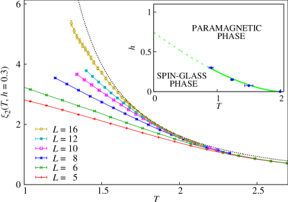
Figure 1: Plot of the second moment correlation length $\xi_{2}$ —eq. (12)— against temperature in an external field $h=0.3$. There is a clear crossover from the convergence to a finite envelope at high $T$ to the more rapid growth at low $T$. As this paper shows, this is caused by the onset of a spin-glass transition. The dotted black line is a fit to a critical divergence as $\xi_{2}^{\infty}\propto[T-T_{\text{c}}(h)]^{-\nu}$, where $T_{\text{c}}$ and $\nu$ are taken from Table 1. The inset is a sketch of the phase diagram (the de Almeida-Thouless line), including a fit to the Fisher-Sompolinsky scaling $h^{2}_{\text{c}}(T)\simeq A|T-T_{\text{c}}^{(0)}|^{\beta^{(0)}+\gamma^{(0)}}$ Fisher and Sompolinsky (1985). The quantities with a superindex $(0)$ are the values for the $h=0$ critical point, Jörg and Katzgraber (2008); Marinari and Zuliani (1999) so the only free parameter is the amplitude $A$.

We have plotted $\xi_{2}$ in Figure 1 for all our lattice sizes and $h=0.3$. There is a clear change of regime from the high-temperature behaviour, where we can see a finite enveloping curve, to the growth of the correlation length at low temperatures. We intend to show that this change of regime actually corresponds to a phase transition, using finite-size scaling Amit and Martin-Mayor (2005).

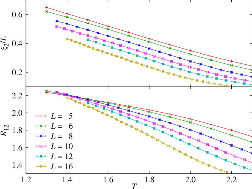
Figure 2: Top: plot of $\xi_{2}/L$ as a function of temperature for all our lattice sizes at $h=0.15$. According to leading-order finite-size scaling, the curves for different sizes should intersect at the phase transition point, but this behaviour is not seen in the plot. This apparent lack of scale invariance has led some authors to conclude that there is no phase transition in this system. Bottom: Same plot of the dimensionless ratio $R_{12}$, eq. (3), which should have the same leading-order scaling as $\xi_{2}/L$. Unlike the correlation length, however, $R_{12}$ does exhibit very clear intersections, signalling the presence of a second-order phase transition. The dramatic improvement in the scaling, compared to the top panel, is explained by the pernicious effect on $\xi_{2}$ of the anomalous behaviour in the correlation function for zero momentum.

In principle, at the transition point there should be scale invariance in the system, meaning that

$$\xi_{2}/L=f_{\xi}\bigl{(}L^{1/\nu}t\bigr{)}+\ldots,\quad t=\frac{T-T_{\text{c}}(h)}{T_{\text{c}}(h)}$$ (2)

where $\nu$ is the thermal critical exponent and the dots represent corrections to leading scaling, expected to be unimportant for large lattice sizes. Therefore, the curves of $\xi_{2}/L$ for large lattices should intersect at the critical point $t=0$. Previous attempts to find $T_{\text{c}}$ using this approach, however, have generally concluded that these intersections cannot be found (or, rather, that the apparent intersection point goes to $T=0$ as $L$ grows) Young and Katzgraber (2004); Jörg et al. (2008). Indeed, if we look at the top panel of Figure 2, we see that either there is no phase transition or $\xi_{2}$ is completely in a preasymptotic regime.

Some authors, working with $D=1$ models with long-range interactions, have already offered an explanation for this apparent lack of scale invariance: the propagator behaves anomalously, but only for the $\boldsymbol{k}=0$ mode Leuzzi et al. (2009). This results in very strong corrections to the leading scaling term of eq. (2), since the second-moment correlation length depends on $\hat{G}(\boldsymbol{k}=0)$. We have checked numerically that this phenomenon is also at play in our $D=4$ system, which is probably a general consequence of the presence of Goldstone bosons in the system (see Appendix B for a discussion of this phenomenon).

In order to avoid this issue, in this paper we take a novel approach, eschewing $\xi_{2}/L$ in favour of a new dimensionless ratio as the basic quantity for our finite-size scaling study. In particular, we shall consider ratios of higher momenta:

$$R_{12}=\frac{\hat{G}(\boldsymbol{k}_{1})}{\hat{G}(\boldsymbol{k}_{2})},$$ (3)

where $\boldsymbol{k}_{1}=(2\pi/L,0,0,0)$, $\boldsymbol{k}_{2}=(2\pi/L,2\pi/L,0,0)$ (and permutations) are the smallest non-zero momenta compatible with the periodic boundary conditions. Notice that, while our use of $R_{12}$ as a basic parameter is novel, this is not in any way a strange quantity. In fact, it is a universal renormalisation-group invariant, whose value in the large-$L$ limit for a paramagnetic system should be $R_{12}(T>T_{\text{c}})=1$. At the critical point, however, $R_{12}(T_{\text{c}})>1$. For instance, using conformal theory relations Di Francesco et al. (1987, 1988), we have computed the critical ratio exactly for the non-disordered $D=2$ Ising model: $R_{12}^{\text{Ising}}(T_{\text{c}})=1.694\,024\ldots$

To leading order, $R_{12}$ should have the same scaling behaviour as $\xi_{2}/L$, namely,

$$R_{12}=f_{12}\bigl{(}L^{1/\nu}t\bigr{)}+\text{[scaling corrections]}.$$ (4)

However, since this quantity avoids the anomalous $\boldsymbol{k}=0$ mode, we expect that corrections to scaling be smaller. Indeed, in the bottom panel of Figure 2 we can see that the improvement in the scaling from the $\xi_{2}$ case is dramatic. Even though corrections to scaling are noticeable, for large sizes the intersections of the curves seem to converge. Notice as well that the high values of $R_{12}$ in the neighbourhood of the intersection point are not only far from the paramagnetic limit of $R_{12}=1$, but also above the bound $R_{12}\leq 2$ that would result from a smooth behaviour of the propagator (see the discussion following eq. (11)).

Therefore, it is our working hypothesis that there is a phase transition, but one that is affected by large corrections to scaling. To substantiate this statement and actually compute the critical parameters, we must begin by somehow controlling these corrections. This analysis is rather technical, but not critical to our discussion, so we leave it for Appendix C, where we study the behaviour of $\xi_{2}/L$ at fixed $R_{12}$ as a function of $L$. To leading order, this should be a constant, so it has allowed us to isolate the effect of the scaling corrections, parameterised as an extra term in $L^{-\omega}$ in (2) and (4), where

$$\omega =1.43(37).$$ (5)

Now that we have the scaling corrections exponent $\omega$, we can go back to study $R_{12}$. The easiest way to compute the critical parameters ($T_{\text{c}}$, $\nu$, etc.) from a renormalisation-group invariant such as $R_{12}$ is the quotients method Ballesteros et al. (1996). Unfortunately, in our case the corrections to scaling are strong, and for some lattice sizes we do not actually reach the intersection point. Let us, therefore, consider an alternative procedure Billoire et al. (2011).

We assume (and therefore will test) that all points of the de Almeida-Thouless line ($h>0$) belong to the same universality class. We begin by considering eq. (4) and explicitely write the corrections to scaling, recall that $t=(T-T_{\mathrm{c}}(h))/T_{\mathrm{c}}(h)$,

$$R_{12}\bigl{(}T,L,h\bigr{)}=f_{12}(tL^{1/\nu})+A(h,tL^{1/\nu})L^{-\omega}+\ldots$$ (6)

Now we define $T_{R}^{L}(h)$ as

$$R_{12}\bigl{(}T_{R}^{L}(h),L,h\bigr{)}=R.$$ (7)

Therefore, if $R$ is in the scaling region, i.e., not too far from $f_{12}(0)$, then

$$T_{R}^{L}(h)\simeq T_{\text{c}}(h)+B_{R,h}L^{-1/\nu}[1+C_{R,h}L^{-\omega}].$$ (8)

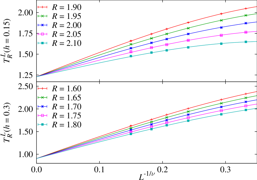
Figure 3: Computation of the critical temperature $T_{\text{c}}(h)$ and the critical exponent $\nu$. We compute the temperature $T_{R}^{L}(h)$ for which $R_{12}(T_{R}^{L},L,h)=R$. For $R$ inside the scaling region, these temperatures should approach the critical one according to (8). We perform a joint fit for all the data sets in the plot, forcing all of them to share the same $\nu$ and forcing all sets with the same $h$ to extrapolate to the same $T_{\text{c}}(h)$. The result of this fit, which had a chi-square per degree of freedom of $\chi^{2}/\text{d.o.f.}=40.2/37$ ($P$-value: 33%), can be seen in Table 1.

Using this formula, keeping $\omega$ fixed to the value of (5), we can, in principle, estimate the critical exponent $\nu$ and the critical temperature $T_{\text{c}}(h)$. However, for a single value of $R$ we do not have enough degrees of freedom in the fit. Therefore, following Álvarez Baños et al. (2010a), we consider several values of $R$ and two values of the field, $h=0.15$ and $h=0.30$ at the same time in a joint fit, where $\nu$ is shared by all data sets and $T_{\text{c}}(h)$ is shared by all the data sets with the same $h$ (see Yllanes (2011) for full details on this fitting procedure). This is plotted in Figure 3, while the fit parameters can be seen in Table 1. We also include the critical temperature for $h=0.075$, extrapolated with the value of $\nu$ computed for $h=0.15$ and $h=0.3$ . We have thus been able to obtain a precise determination of $T_{\text{c}}(h)$ and of the critical exponent $\nu$. It is important to mention that the value of $\nu$ which, as we have seen, is universal for $h>0$, is very different from that of the $h=0$ case. As a consistency check of our non-standard finite-size scaling method, we have run a smaller set of simulations for $h=0$ and obtained $\nu^{(0)}=0.96(11)$ and $T_{\mathrm{c}}^{(0)}=2.002(10)$, in good agreement with previous results for the $h=0$ case Jörg and Katzgraber (2008); Marinari and Zuliani (1999). We remark that both the critical temperature and $\nu^{(0)}$ widely differ from the values in Table 1.

Parameter	$h=0.3$	$h=0.15$	$h=0.075$
$T_{\text{c}}(h)$	0.906(40)[3]	1.229(30)[2]	1.50(7)
$\nu$	1.46(7)[6]		—
$\eta$	$-0.30(4)[1]$		—

Table 1: Critical temperatures and exponents for our model. The second error bar, in square brackets, refers to the effect of the uncertainty in $\omega$. In order to compute $\nu$ and $T_{\text{c}}(h)$ we studied the scaling of $R_{12}$ with a joint fit for $h=0.15$ and $h=0.3$, as depicted in Figure 3. The value of $\eta$ was computed from the scaling of $\hat{G}(\boldsymbol{k})$ at $h=0.15$ and $h=0.3$. The data for $h=0.075$ presented severe corrections, probably due to the proximity of the $h=0$ critical point. Therefore, we did not include this field in the previous fits and only used the data for $L\geq 12$ in order to estimate $T_{\text{c}}(h=0.075)$ using the previously computed $\nu$.

The determination of the second independent critical exponent, the anomalous dimension $\eta$ of the propagator, is much more difficult. In principle, we could consider the scaling of the propagator $\hat{G}(\boldsymbol{k})$ at fixed $R_{12}=R$. However, $\eta$ is more affected by the scaling corrections than $\nu$. In fact, as discussed in Appendix C, we had to consider quadratic corrections to scaling, as $A_{1}L^{-\omega_{\text{eff}}}+A_{2}L^{-2\omega_{\text{eff}}}$, with $\omega_{\text{eff}}=2.2(3)$, in order to fit the data. Our final estimate is quoted in Table 1. Finally, we can combine our results in Table 1 to sketch the de Almeida-Thouless line. This is plotted in the inset to Figure 1, where we also show a very good fit to the Fisher-Sompolinsky scaling Fisher and Sompolinsky (1985).

Let us finally mention that one may analyse our data as well under the assumption of the absence of the phase transition in a field. This analysis, which relies on Refs. Fisher and Huse (1988); Hartmann (1999); Hukushima (1999), is reported in Appendix D. The data fail to follow basic scaling relations derived under the no-transition hypothesis (or, at least, they fail to scale within the range of system sizes that we could simulate).

II Discussion

In summary, we have presented a finite-size scaling study of the four dimensional Edwards-Anderson model of an Ising spin glass in an external magnetic field. We have been able to reach large system sizes and low temperatures, thanks to the Janus special-purpose computer. We introduce a novel finite-size scaling method, which cures the anomalies first observed in Leuzzi et al. (2009). We present conclusive evidence for the presence of a de Almeida-Thouless line in the temperature-magnetic field phase plane (inset for Figure 1), whose universality class we characterise. In other words, a spin-glass transition occurs, even without time-reversal symmetry, for realistic models (i.e., well below the upper critical dimension $d_{\mathrm{u}}=6$). A far-reaching consequence is that the universality class for the phase transition in structural glasses may actually exist Moore and Drossel (2002). Our result also settles a longstanding controversy in the field of spin glasses (see, e.g., Bray and Moore (2011); Parisi and Temesvári (2011)).

Appendix A Simulations

$L$	$h$	$T_{\mathrm{min}}$	$T_{\mathrm{max}}$	$N_{T}$	$N_{\text{s}}$
$5$	$0.075$	$1.300$	$2.600$	$14$	$25600$
$5$	$0.150$	$1.300$	$2.600$	$14$	$25600$
$5$	$0.300$	$0.833$	$2.797$	$20$	$25600$
$6$	$0.075$	$1.300$	$2.600$	$14$	$25600$
$6$	$0.150$	$1.300$	$2.600$	$14$	$25600$
$6$	$0.300$	$0.833$	$2.797$	$20$	$25600$
$8$	$0.075$	$1.350$	$2.500$	$24$	$25600$
$8$	$0.150$	$1.350$	$2.500$	$24$	$25600$
$8$	$0.300$	$1.200$	$2.325$	$16$	$25600$
$10$	$0.075$	$1.350$	$2.402$	$26$	$25600$
$10$	$0.150$	$1.350$	$2.402$	$26$	$25600$
$10$	$0.300$	$1.340$	$2.243$	$20$	$25600$
$12$	$0.075$	$1.425$	$2.402$	$24$	$25600$
$12$	$0.150$	$1.502$	$2.402$	$22$	$12800$
$12$	$0.3$	$1.400$	$2.160$	$20$	$25600$
$16$	$0.075$	$1.400$	$2.179$	$32$	$4000$
$16$	$0.15$	$1.400$	$2.179$	$32$	$4000$
$16$	$0.300$	$1.304$	$1.681$	$18$	$1000$

Table 2: Parameters describing our parallel tempering simulations. The $N_{T}$ temperatures were evenly spaced between $T_{\mathrm{min}}$ and $T_{\mathrm{max}}$ for $L\leq 12$, but with a slightly larger separation in the hot region for $L=16$. We simulate four real replicas for each of the $N_{\mathrm{s}}$ samples.

We have carried out parallel tempering Hukushima and Nemoto (1996); Marinari (1998) simulations for three values of the magnetic field (see Table 2), with periodic boundary conditions.

Our thermalisation protocol is sample dependent (see Yllanes (2011) for details). We first perform a number of iterations large enough to ensure thermalisation in a large fraction of the samples (typically 90%). We study the autocorrelation of the temperature flow during the parallel tempering and extend the runs for the slower samples until a total length of 14 exponential autocorrelation times is ensured. The final product is a set of thermalised and almost independent configurations. As an example, each $L=16$ sample in $h=0.15$ was simulated at least for $5\times 10^{7}$ heat bath lattice sweeps at each of the $N_{T}=32$ temperatures (we performed a parallel tempering update every 10 heat baths). However, the hardest sample required as many as $2.6\times 10^{10}$ heat bath sweeps.

The $L=16$ lattices were simulated on the Janus computer with an update speed (for each of its 256 units) of $86$ ps per spin flip with a heat bath scheme. The $L\leq 12$ lattices were simulated on PC clusters, with a C code that uses multi-spin coding Newman and Barkema (1999) with 128-bit words (using the SSE extensions); the update speed in this case is 350 ps per spin flip using a Metropolis algorithm (on an Intel Core2 processor at 2.40GHz) With multi-spin coding, the samples whose simulations have to be extended must be extracted from the original 128-sample bundles to construct new bundles that are then extended with the same code. Note finally that, since the PC spreads the spin-flips over 128 samples, the simulation for each sample is faster on Janus by a factor $\sim 500$. This difference is significant when the equilibration time is large.

Appendix B The correlation functions

The main quantities that we compute are the correlation functions. In the presence of a magnetic field, the expectation of each spin $S_{\boldsymbol{x}}$ is non-vanishing. Hence we may consider these two correlation functions:

$$G_{1}(\boldsymbol{r}) = \frac{1}{L^{4}}\sum_{\boldsymbol{x}}\overline{\bigl{(}\langle S_{\boldsymbol{x}}S_{\boldsymbol{x}+\boldsymbol{r}}\rangle-\langle S_{\boldsymbol{x}}\rangle\langle S_{\boldsymbol{x}+\boldsymbol{r}}\rangle\bigr{)}^{2}}\,,$$ (9)

$$G_{2}(\boldsymbol{r}) = \frac{1}{L^{4}}\sum_{\boldsymbol{x}}\overline{\bigl{(}\langle S_{\boldsymbol{x}}S_{\boldsymbol{x}+\boldsymbol{r}}\rangle^{2}-\langle S_{\boldsymbol{x}}\rangle^{2}\langle S_{\boldsymbol{x}+\boldsymbol{r}}\rangle^{2}\bigr{)}}\,.$$ (10)

In the above, the $\langle\cdots\rangle$ stands for the thermal average in a single sample, while the disorder average is indicated by an overline. Note that the Fourier transform $\hat{G}_{1}(\boldsymbol{k}=0)$ is the spin-glass susceptibility. We simulate four real replicas $\{S_{\boldsymbol{x}}^{(a)}\}$ (i.e., four systems with the same coupling evolving independently under the thermal noise) in order to obtain unbiased estimators of the correlation functions. In the main text $G$ stands for either of the $G_{1,2}$. In the fits we have combined data from both whenever it was useful to obtain smaller statistical errors.

The correlation functions were computed off-line over stored configurations. We note that configurations at different Monte Carlo times can be combined as long as they belong to different replicas Álvarez Baños et al. (2010b). This results in small Monte Carlo errors with a modest number of configurations, so the uncertainty on the final result is dominated by the sample-to-sample fluctuations. This step is rather time consuming, so we also use multi-spin coding to accomplish it.

In order to define the second-moment correlation length Cooper et al. (1982), we consider the following Ornstein-Zernike expansion for the propagator in Fourier space,

$$\frac{1}{\hat{G}(\boldsymbol{k})}=\frac{\xi^{2}}{\hat{G}(0)}\left[\frac{1}{\xi^{2}}+\cancel{k}^{2}+a_{4}(\cancel{k}^{2})^{2}+\ldots\right],$$ (11)

where $\cancel{k}^{2}=4\sum_{\mu}\sin^{2}(k_{\mu}/2)$. Then, the common second-moment correlation length $\xi_{2}$ is obtained by truncating the expansion at the $\cancel{k}^{2}$ term:

$$\xi_{2}=\frac{1}{2\sin(\pi/L)}\left(\frac{\hat{G}(0)}{\hat{G}(\boldsymbol{k}_{1})}-1\right)^{1/2},$$ (12)

As we comment in the main text, this definition is not well behaved for our model, due to the anomalous behaviour of the $\boldsymbol{k}=0$ mode. Actually, there is a simple, yet unexpected explanation for this anomaly. It arises whenever soft excitations (Goldstone bosons) are present in the low-temperature phase, while an external magnetic field splits excitations into longitudinal and transversal Zinn-Justin (2005). Familiar examples of Goldstone bosons are magnons, or the phonons in an acoustical branch. What is most peculiar about spin glasses is that soft modes are present Bray and Moore (1987); de Dominicis et al. (1998), even if our variables are discrete.

Appendix C Computation of the scaling corrections

In order to compute corrections to scaling, we recall that the behavior of $\xi_{2}/L$ and $R_{12}$ is the same to leading scaling order:

$$\xi_{2}/L(T,L,h) =f_{\xi}(tL^{1/\nu})+\text{[scaling corrections]},$$ (13)

$$R_{12}(T,L,h) =f_{12}(tL^{1/\nu})+\text{[scaling corrections]}.$$ (14)

As we saw in Figure 2, the effect of the scaling corrections was dramatic for $\xi_{2}/L$ (they erase all trace of a phase transition in the simulated regime). For $R_{12}$, the deviation from the leading scaling was milder, but still strong enough that we cannot ignore it in our analysis. Therefore, it becomes necessary to parameterize the corrections.

Since the number of lattice sizes is not enough to fit for the leading order behavior and the corrections at the same time, our strategy has been isolating the latter. In order so to do, we first consider the evolution of $\xi_{2}/L$ as a function of $R_{12}$ (Figure 4). According to (13), to leading order this function should not depend on the lattice size. We see in the figure that this behavior is indeed realized at high temperatures (low values of $R_{12}$) but that, close to the transition point, the deviations become very strong. Therefore, by fixing the value of $R_{12}$ and studying the evolution of $\xi_{2}/L$ with the system size we can isolate the corrections to scaling. These include an enormous variety of effects, but the standard practice is to consider simply the leading corrections, characterized by an exponent $\omega$

$$\begin{split}\xi_{2}(T,L,h)/L\simeq&g\bigl{(}R_{12}(T,L,h)\bigr{)}\\ &+A\bigl{(}R_{12}(T,L,h),h\bigr{)}L^{-\omega}.\end{split}$$ (15)

Notice that the extrapolation to infinite volume depends only on $R_{12}$, but that the amplitude of the corrections depends also separately on the magnetic field $h$. We can, therefore, consider a joint fit to (15) for $h=0.15,0.3$ and several values of $R_{12}$. Data for $h=0.075$ are not included due to their proximity to $h=0$. In this global fit, the value of $\omega$ is shared by all data sets, while the infinite-volume extrapolation is common to the data sets with the same $R_{12}$ but different $h$. This is represented in Figure 5, where we only show a few $R_{12}$ values for clarity. In this computation we use our data for $L>10$. The result and the chi-square per degree of freedom (as well as the $P$-value of the fit) are

$$\omega =1.43(37), \chi^{2}/\text{d.o.f.} =9.2/11\ (P=60\%).$$ (16)

This is the value of $\omega$ used in the main text of the paper to compute $\nu$ and the critical temperatures. Notice, however, that for its computation we had to restrict the fit to lattice sizes $L\geq 12$. For smaller systems, the effect of subleading corrections to scaling is very important, as evinced by the curvature in the plots of the figure.

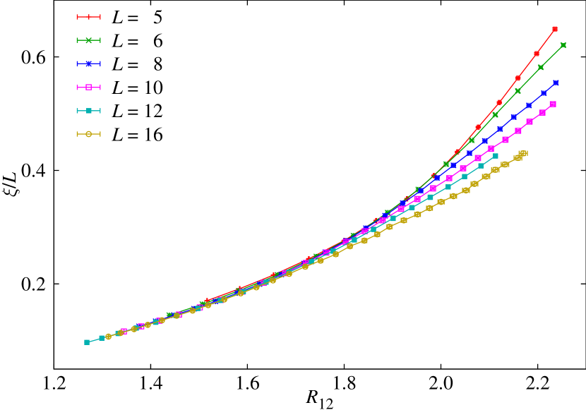
Figure 4: Plot of $\xi_{2}/L$ against $R_{12}$ at $h=0.15$. To leading scaling order, this curve should be independent of the system size, a prediction that is realized at low values of $R_{12}$ (i.e., far from the critical point). Close to the critical point, however, strong scaling corrections appear.

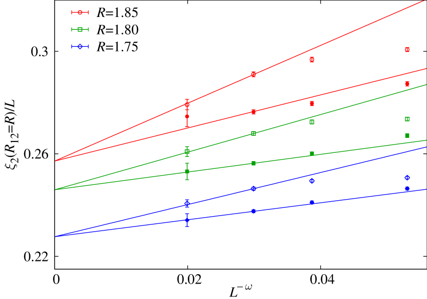
Figure 5: Plots of $\xi_{2}/L$ at fixed $R_{12}=R$ as a function of the lattice size (i.e., vertical cuts of the left panel) for $h=0.15$ (empty symbols) and $h=0.3$ (solid symbols). The extrapolation to the $h$-independent limit for each $R$ is governed by the scaling corrections exponent $\omega$ —eq. 15 . We have performed a joint fit for several values of $R$, forcing all data sets to share the same exponent and taking their correlation into account

Since this is a potentially dangerous effect, we have also, as a consistency check, tried to include smaller lattices in the fit at the cost of including more correction terms. Unfortunately, these subleading corrections are extremely varied and we cannot be sure of the relative importance of each term. We do know, however, that among them is a series on powers of $L^{-\omega}$. Therefore, we can consider an effective parameterization of the corrections in the following way

$$\begin{split}\xi_{2}(T,L,h)/L\simeq&g\bigl{(}R_{12}(T,L,h)\bigr{)}\\ &+B\bigl{(}R_{12}(T,L,h),h\bigr{)}L^{-\omega_{\text{eff}}}\\ &+C\bigl{(}R_{12}(T,L,h),h\bigr{)}L^{-2\omega_{\text{eff}}}.\end{split}$$ (17)

If we redo the computation of Figure 5 in this non-standard way, including lattices with $L>6$ we obtain a value of $\omega_{\text{eff}}=2.2(3)$. At a first glance the discrepancy with the previous $\omega$ may seem alarming. Actually, a computation of $\nu$ and the critical temperatures with this alternative corrections to scaling yields compatible values: $T_{\text{c}}(0.3)=0.902(33)[1],$ $T_{\text{c}}(0.15)=1.233(23)[1]$ and $\nu=1.54(6)[2]$, with $\chi^{2}/\text{d.o.f.}=39.0/37$ $(P=38\%)$. This can be seen as a check that, even though the scaling corrections are strong, our computation of the critical parameters is robust.

A final comment regards the estimation of the second independent critical exponent, $\eta$. We can consider the scaling of the propagator $\hat{G}(\boldsymbol{k})$ at fixed $R_{12}=y$ (i.e., at $T=T_{y}^{L}$, see main text), with either of the two models for the scaling corrections:

$$\hat{G}(\boldsymbol{k},T_{y}^{L},L,h) \simeq A_{k,h,y}L^{2-\eta}[1+B_{k,h,y}L^{-\omega}].$$ (18)

$$\hat{G}(\boldsymbol{k},T_{y}^{L},L,h) \simeq A_{k,h,y}L^{2-\eta}[1+C_{k,h,y}L^{-\omega_{\text{eff}}}$$ (19)

$$\hskip 81.09052ptD_{k,h,y}L^{-2\omega_{\text{eff}}}].$$

In this case we have found that the first form, including only the leading corrections, does not adequately represent our data unless we exclude from the fit so many lattice sizes that we lose all degrees of freedom. Therefore, we cannot make a controlled determination of this critical exponent using (18). The most that can be said is that the propagator $\hat{G}(\boldsymbol{k})$ —and, in particular, the susceptibility $\tilde{\chi}=\hat{G}(0)$— diverges quickly at the critical point, with a value of $\eta\approx-0.3$, similar to the value for $h=0$.

On the other hand, using the effective quadratic corrections of (C), the value of this exponent results

$$\eta =-0.30(4)[1],$$ (20)

with $\chi^{2}/\text{d.o.f.}=9.55/11$ ($P=57\%$). This is the value quoted in Table 1 of the paper.

Appendix D The no-transition hypothesis

Let us assume that no real phase transition arises in a field. For the sake of brevity, we introduce the reduced temperature, which depends on the standard temperature $T$:

$$t=\frac{T-T_{\mathrm{c}}}{T_{\mathrm{c}}}\,.$$ (21)

In particular, note that $t(T_{\mathrm{c}})\!=\!0$, while $t(T\!=\!0)\!=\!-1$. In this section, we are assuming that the only phase transition occurs when $h=0$, hence $T_{\mathrm{c}}$ refers to the zero-field critical temperature. Therefore, in a field, the correlation length in the thermodynamic limit is finite for all temperatures: $\xi(t,h)<\infty$ if $h>0$. Under these circumstances, it is unavoidable that

$$\lim_{L\to\infty}R_{12}(t,h,L)=1\,.$$ (22)

Nevertheless, it is quite reasonable to expect that $R_{12}$ verify a scaling law ($W$ is a scaling function):

$$R_{12}(t,h,L)=W(\xi(t,h)/L)$$ (23)

In order to model our data according to this expectation, we need some educated guess for $\xi(t,h)$. We shall get it from the droplet model for spin glasses Bray and Moore (1987); Fisher and Huse (1988).

We first gather some necessary information in Sects. D.1 and D.2. Our data are analyzed under this light in Sect. D.3.

D.1 The critical behavior according to the droplet model

In the droplet model for spin glasses Fisher and Huse (1988), one expects for $t=-1$ (i.e. $T=0$) a correlation length that diverges only in the limit of $h\to 0$:

$$\xi(t=-1,h)\propto h^{-2/(D-2\theta)}\,,$$ (24)

where $\theta$ is the droplet exponent. In $D=4,$ that exponent is $\theta\approx 0.7$ Hartmann (1999); Hukushima (1999). So, the prediction is

$$\xi_{\mathrm{droplet}}(t=-1,h)\propto 1/h^{0.77}\,.$$ (25)

Fisher and Huse Fisher and Huse (1988), define as well a dynamical de Almeida-Thouless (dAT) line. That is, a freezing temperature which should scale very much as the equilibrium dAT line (which is inexistent on their theory). This freezing line $T_{f}(t_{m},h)$ would depend on the measuring time $t_{m}$ as ($\tau_{0}$ is a microscopic time unit and $\Psi$ is the barrier exponent)

$$\frac{T_{\mathrm{c}}-T_{f}(t_{m},h)}{T_{\mathrm{c}}}\sim h^{\frac{2}{\gamma+\beta}}[\log(t_{m}/\tau_{0})]^{(D-\theta)/(\gamma+\beta)\Psi}\,.$$ (26)

Hence, for a fixed measuring time $t_{m}$, the freezing line scales with $h$ just as expected for the dAT line, see Sect. D.2 below.

Fisher and Huse description Fisher and Huse (1988) of the crossover phenomena to be observed in equilibrium, coincides with our Eq. (37) (see below).

D.2 Scaling close to the $h=0$ critical point

The critical behavior of the Edwards-Anderson model, in $D=4$ and $h=0$, is relatively well understood Jörg and Katzgraber (2008); Marinari and Zuliani (1999):

$$T_{\mathrm{c}}=2.03(3)\,,$$ (27)

$$\nu=1.025(15)\,,$$ (28)

$$\eta=-0.275(25)\,.$$ (29)

From these estimates, we obtain the Renormalization Group (RG) eigenvalues $y_{t}$ and $y_{h}$,

$$y_{t} =1/\nu=0.976(14)\,,$$ (30)

$$y_{h} =\frac{D+2-\eta}{2}=3.137(13)\,.$$ (31)

In order to make connection with Eq. (26), note, in particular, that $y_{t}/y_{h}=1/(\beta+\gamma)$.

The Fisher-Sompolinski relation Fisher and Sompolinsky (1985), follows from a simple scaling argument. Recall that, for spin glasses, the ordering field is $h^{2}$ rather than $h$, due to the gauge invariance of the coupling distribution. Hence, the RG transformation of scale $b$ transforms $h^{2}$ into $b^{y_{h}}h^{2}$, while the correlation length transforms as (see, e.g., Amit and Martin-Mayor (2005))

$$\xi(t,h)=b\,\xi(b^{y_{t}}t,b^{y_{h}/2}h)\,.$$ (32)

Let us now choose $b$ such that $b^{y_{h}}h^{2}=1$, hence

$$\xi(t,h^{2})=\frac{1}{h^{2/y_{h}}}G(t/h^{2y_{t}/y_{h}})\,,$$ (33)

where $G(x)$ is a scaling function. Now, imagine that there is a dAT line. Then, one should be able of adjusting the temperature, at fixed $h>0$, in such a way that $\xi(t,h)$ grows unboundly. On the view of Eq. (33), this is only possible if the scaling function $G(x)$ has a singularity at some $x^{*}$. Hence, the dAT line would be located at

$$t=x^{*}h^{2y_{t}/y_{h}}=x^{*}h^{2/(\beta+\gamma)}\,,$$ (34)

at least while the scaling fields $t$ and $h$ are small enough to behave linearly under the RG, as we have assumed in Eq. (32).

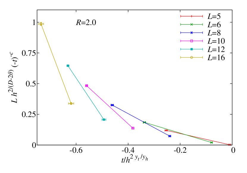
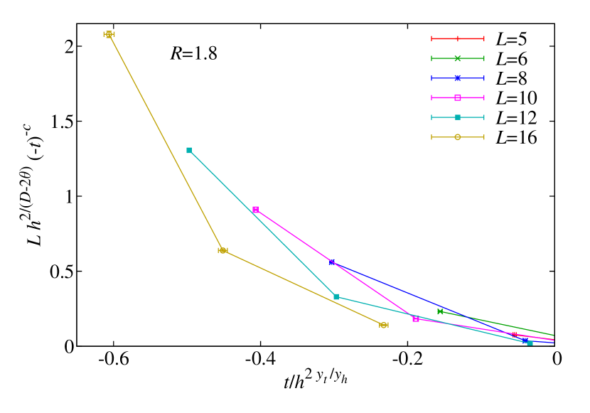
Figure 6: Numerical test of Eq. (39). For every lattice size $L$, and fields $h$, we obtain the temperature where $R_{12}(T_{R}^{L},L,h)=R$. The reduced temperature $t_{R}^{L}(h)$ is computed through Eq. (21) ($T_{\mathrm{c}}$ is the zero-field critical temperature). According to the droplet model, and neglecting scaling corrections, for fixed $R$, $Lh^{2/(D-2\theta)}[-t_{R}^{L}(h)]^{c}$ must be an $L$-independent function of $t_{R}^{L}(h)/h^{2y_{t}/y_{h}}$. We plot data for $R=2$ (top), and $R=1.8$ (bottom). For $R=2.0$, $T_{R}^{L}$ lies within our simulated temperature trange only for $h=0.15,0.075$. In the plot, we used $\theta=0.7$, which is an average among $\theta=0.65$ (from Hartmann (1999)), and $\theta=0.82$ (from Hukushima (1999)). No matter the value that we take for $\theta$ in this range, $Lh^{2/(D-2\theta)}[-t_{R}^{L}(h)]^{c}$ grows quickly with $L$ and draws an increasingly steep curve.

D.3 The ansatz for $\xi(t,h)$ and the comparison with numerical data

As said above, we need some educated guess about the behavior of $\xi(T,h)$ in the droplet picture. We take inspiration from Eqs. (33) and (24).

Of course, the scaling function $G(x)$ in Eq. (33) must be regular for all $x$ because, according to the droplet picture, there is no phase transition. However, the function $G(x)$ must be singular for $x\to-\infty$ (which corresponds to taking first the limit $T\to 0$, i.e. $t=-1$, and later the limit $h\to 0$). In fact, if $G(x)$ would tend to a constant for large, negative $x$, one would have $\xi(T=0,h)\sim 1/h^{2/y_{h}}\approx 1/h^{0.64}$. This is inconsistent with Eq. (25) (i.e. $\xi\propto 1/h^{0.77}$). Nevertheless, a mild singularity $G(x\to-\infty)\sim(-x)^{c}$, where exponent $c$ verifies

$$\frac{2}{y_{h}}(y_{t}c+1)=\frac{2}{D-2\theta}$$ (35)

would make equation (33) consistent with Eq. (24). Solving for $c$, we get

$$c=\frac{y_{h}-D+2\theta}{y_{t}(D-2\theta)}\approx 0.21$$ (36)

Hence, our ansatz for $\xi(t,h)$, inspired by the droplet theory, is

$$\xi_{\mathrm{ansatz}}(t,h)=\frac{(-t)^{c}}{h^{\frac{2}{D-2\theta}}}F(t/h^{2y_{t}/y_{h}})\,.$$ (37)

The new scaling function is $F(x)=G(x)/(-x)^{c}$. $F(x)$ should remain finite in the limit $x\to-\infty$ (note, however, that $F(x)\sim 1/(-x)^{c}$ for $x\approx 0$, which corresponds to the neighborhood of $T_{\mathrm{c}}$).

Plugging $\xi_{\mathrm{ansatz}}(t,h)$ in (23), we get

$$\begin{split}R_{12}(t,h,L)&=W(\xi_{\mathrm{ansatz}}(t,h)/L)\\ &=W\left(\frac{(-t)^{c}}{Lh^{2/(D-2\theta)}}F(t/h^{2y_{t}/y_{h}})\right)\,.\end{split}$$ (38)

Now, in the main text we paid great attention to $T_{R}^{L}(h)$, namely the temperature where $R_{12}(T_{R}^{L},L,h)=R$ (one may compute easily the reduced temperature $t_{R}^{L}(h)$). We thus recast Eq. (38) in a form directly amenable to a scaling analysis:

$$Lh^{2/(D-2\theta)}[-t_{R}^{L}(h)]^{c}W^{-1}(R)=F\left(\frac{t_{R}^{L}(h)}{h^{2y_{t}/y_{h}}}\right)\,,$$ (39)

where $W^{-1}(x)$ is the inverse function of $W(x)$.

Hence, the prediction of the droplet model is fairly simple. For fixed $R$, and barring scaling corrections (negligible for large $L$), the numerical estimate of the l.h.s., namely $Lh^{2/(D-2\theta)}[-t_{R}^{L}(h)]^{c}$, must be an $L$-independent function of $t_{R}^{L}(h)/h^{2y_{t}/y_{h}}$. On the other hand, if a phase transition occurs at fixed $t(h)/h^{2y_{t}/y_{h}}$ (as claimed in the main text), $t_{R}^{L}(h)$ should tend to $t(h)$ while the l.h.s. should diverge as $L$ grows. In other words, if there is a dAT line, data should tend to a vertical line in the large $L$ limit.

These two alternatives are compared in Figure 6. In fact, our estimate for $Lh^{2/(D-2\theta)}[-t_{R}^{L}(h)]^{c}$ grows fast with $L$ and draws an increasingly steep curve, which is the behavior expected in the presence of a dAT line. This is hardly surprising, because the numerical data in Figure 2–bottom, where $R_{12}$ shows scale invariant behavior, are plainly inconsistent with our starting assumption in Eq. (22).

In summary, either our simulated sizes are entirely in a preasymptotic regime, or the no-transition hypothesis is not realized.

References

- Debenedetti (1997) P. G. Debenedetti, Metastable Liquids (Princeton University Press, Princeton, 1997).
- Debenedetti and Stillinger (2001) P. G. Debenedetti and F. H. Stillinger, Nature 410, 259 (2001).
- Cavagna (2009) A. Cavagna, Physics Reports 476, 51 (2009), arXiv:0903.4264 .
- Mydosh (1993) J. A. Mydosh, Spin Glasses: an Experimental Introduction (Taylor and Francis, London, 1993).
- Hérisson and Ocio (2002) D. Hérisson and M. Ocio, Phys. Rev. Lett. 88, 257202 (2002), arXiv:cond-mat/0112378 .
- Cruz et al. (2001) A. Cruz, J. Pech, A. Tarancon, P. Tellez, C. L. Ullod, and C. Ungil, Comp. Phys. Comm 133, 165 (2001), arXiv:cond-mat/0004080 .
- Ogielski (1985) A. Ogielski, Phys. Rev. B 32, 7384 (1985).
- Belletti et al. (2008a) F. Belletti, M. Cotallo, A. Cruz, L. A. Fernandez, A. Gordillo, A. Maiorano, F. Mantovani, E. Marinari, V. Martin-Mayor, J. Monforte, A. Muñoz Sudupe, D. Navarro, S. Perez-Gaviro, J. J. Ruiz-Lorenzo, S. F. Schifano, D. Sciretti, A. Tarancon, R. Tripiccione, and J. L. Velasco (Janus Collaboration), Comp. Phys. Comm. 178, 208 (2008a), arXiv:0704.3573 .
- Belletti et al. (2008b) F. Belletti, M. Cotallo, A. Cruz, L. A. Fernandez, A. Gordillo-Guerrero, M. Guidetti, A. Maiorano, F. Mantovani, E. Marinari, V. Martin-Mayor, A. Muñoz Sudupe, D. Navarro, G. Parisi, S. Perez-Gaviro, J. J. Ruiz-Lorenzo, S. F. Schifano, D. Sciretti, A. Tarancon, R. Tripiccione, J. L. Velasco, and D. Yllanes (Janus Collaboration), Phys. Rev. Lett. 101, 157201 (2008b), arXiv:0804.1471 .
- Gunnarsson et al. (1991) K. Gunnarsson, P. Svendlindh, P. Nordblad, L. Lundgren, H. Aruga, and A. Ito, Phys. Rev. B 43, 8199 (1991).
- Ballesteros et al. (2000) H. G. Ballesteros, A. Cruz, L. A. Fernandez, V. Martin-Mayor, J. Pech, J. J. Ruiz-Lorenzo, A. Tarancon, P. Tellez, C. L. Ullod, and C. Ungil, Phys. Rev. B 62, 14237 (2000), arXiv:cond-mat/0006211 .
- Palassini and Caracciolo (1999) M. Palassini and S. Caracciolo, Phys. Rev. Lett. 82, 5128 (1999), arXiv:cond-mat/9904246 .
- Bray and Moore (2011) A. J. Bray and M. A. Moore, Phys. Rev. B 83, 224408 (2011), arXiv:1102.1675 .
- Parisi and Temesvári (2011) G. Parisi and T. Temesvári, (2011), arXiv:1111.3313 .
- Bray and Roberts (1980) A. J. Bray and S. A. Roberts, J. Phys. C: Solid St.Phys. 13, 5405 (1980).
- de Almeida and Thouless (1978) J. R. L. de Almeida and D. J. Thouless, J. Phys. A 11, 983 (1978).
- Note (1) A more careful analysis is needed in order to reach the same conclusion in the range Fisher and Sompolinsky (1985).
- Young and Katzgraber (2004) A. P. Young and H. G. Katzgraber, Phys. Rev. Lett. 93, 207203 (2004), arXiv:cond-mat/0407031 .
- Jörg et al. (2008) T. Jörg, H. Katzgraber, and F. Krzakala, Phys. Rev. Lett. 100, 197202 (2008), arXiv:0712.2009 .
- Jönsson et al. (2005) P. E. Jönsson, H. Takayama, H. Aruga Jatori, and A. Ito, Phys. Rev. B 71, 180412(R) (2005), arXiv:cond-mat/0411291 .
- Petit et al. (1999) D. Petit, L. Fruchter, and I. Campbell, Phys. Rev. Lett 83, 5130 (1999), arXiv:cond-mat/9910353 .
- Petit et al. (2002) D. Petit, L. Fruchter, and I. Campbell, Phys. Rev. Lett 88, 207206 (2002), arXiv:cond-mat/011112 .
- Tabata et al. (2010) Y. Tabata, K. Matsuda, S. Kanada, T. Yamazaki, T. Waki, H. Nakamura, K. Sato, and K. Kindo, Journal of Physical Society of Japan 79, 123704 (2010), arXiv:1009.6115 .
- Moore and Drossel (2002) M. Moore and B. Drossel, Phys. Rev. Lett. 89, 217202 (2002), arXiv:cond-mat/0201107 .
- Leuzzi et al. (2009) L. Leuzzi, G. Parisi, F. Ricci-Tersenghi, and J. J. Ruiz-Lorenzo, Phys. Rev. Lett. 103, 267201 (2009), arXiv:0811.3435 .
- Fisher and Sompolinsky (1985) D. S. Fisher and H. Sompolinsky, Phys. Rev. Lett. 54, 1063 (1985).
- Jörg and Katzgraber (2008) T. Jörg and H. G. Katzgraber, Phys. Rev. B 77, 214426 (2008), arXiv:0803.3339 .
- Marinari and Zuliani (1999) E. Marinari and F. Zuliani, J. Phys. A 32, 7447 (1999), arXiv:cond-mat/9904303 .
- Amit and Martin-Mayor (2005) D. J. Amit and V. Martin-Mayor, Field Theory, the Renormalization Group and Critical Phenomena, 3rd ed. (World Scientific, Singapore, 2005).
- Di Francesco et al. (1987) P. Di Francesco, H. Saleur, and J.-B. Zuber, Nucl. Phys. B 290, 527 (1987).
- Di Francesco et al. (1988) P. Di Francesco, H. Saleur, and J.-B. Zuber, Europhys. Lett. 5, 95 (1988).
- Ballesteros et al. (1996) H. G. Ballesteros, L. A. Fernandez, V. Martin-Mayor, and A. Muñoz Sudupe, Phys. Lett. B 378, 207 (1996), arXiv:hep-lat/9511003 .
- Billoire et al. (2011) A. Billoire, L. A. Fernandez, A. Maiorano, E. Marinari, V. Martin-Mayor, and D. Yllanes, J. Stat. Mech. (2011), P10019, arXiv:1108.1336 .
- Álvarez Baños et al. (2010a) R. Álvarez Baños, A. Cruz, L. A. Fernandez, J. M. Gil-Narvion, A. Gordillo-Guerrero, M. Guidetti, A. Maiorano, F. Mantovani, E. Marinari, V. Martin-Mayor, J. Monforte-Garcia, A. Muñoz Sudupe, D. Navarro, G. Parisi, S. Perez-Gaviro, J. Ruiz-Lorenzo, S. F. Schifano, B. Seoane, A. Tarancon, R. Tripiccione, and D. Yllanes (Janus Collaboration), Phys. Rev. Lett. 105, 177202 (2010a), arXiv:1003.2943 .
- Yllanes (2011) D. Yllanes, Rugged Free-Energy Landscapes in Disordered Spin Systems (Ph.D. thesis, UCM, 2011) arXiv:1111.0266 .
- Note (2) The data for presented very severe corrections, probably due to the proximity of the critical point. Therefore, we only use the data for in order to estimate .
- Fisher and Huse (1988) D. S. Fisher and D. A. Huse, Phys. Rev. B 38, 373 (1988).
- Hartmann (1999) A. K. Hartmann, Phys. Rev. E. 60, 5135 (1999), arXiv:cond-mat/9904296 .
- Hukushima (1999) K. Hukushima, Phys. Rev. E 60, 3606 (1999), arXiv:cond-mat/9903391 .
- Hukushima and Nemoto (1996) K. Hukushima and K. Nemoto, J. Phys. Soc. Japan 65, 1604 (1996), arXiv:cond-mat/9512035 .
- Marinari (1998) E. Marinari, in Advances in Computer Simulation, edited by J. Kerstész and I. Kondor (Springer-Berlag, 1998).
- Newman and Barkema (1999) M. E. J. Newman and G. T. Barkema, Monte Carlo Methods in Statistical Physics (Clarendon Press, Oxford, 1999).
- Álvarez Baños et al. (2010b) R. Álvarez Baños, A. Cruz, L. A. Fernandez, J. M. Gil-Narvion, A. Gordillo-Guerrero, M. Guidetti, A. Maiorano, F. Mantovani, E. Marinari, V. Martin-Mayor, J. Monforte-Garcia, A. Muñoz Sudupe, D. Navarro, G. Parisi, S. Perez-Gaviro, J. Ruiz-Lorenzo, S. F. Schifano, B. Seoane, A. Tarancon, R. Tripiccione, and D. Yllanes (Janus Collaboration), J. Stat. Mech. (2010), P06026 , arXiv:1003.2569 .
- Cooper et al. (1982) F. Cooper, B. Freedman, and D. Preston, Nucl. Phys. B 210, 210 (1982).
- Zinn-Justin (2005) J. Zinn-Justin, Quantum Field Theory and Critical Phenomena, 4th ed. (Clarendon Press, Oxford, 2005).
- Bray and Moore (1987) A. J. Bray and M. A. Moore, in Heidelberg Colloquium on Glassy Dynamics, Lecture Notes in Physics No. 275, edited by J. L. van Hemmen and I. Morgenstern (Springer, Berlin, 1987).
- de Dominicis et al. (1998) C. de Dominicis, I. Kondor, and T. Temesvári, in Spin Glasses and Random Fields, edited by A. P. Young (World Scientific, Singapore, 1998).