Using an Ellipsoid Model to Track and Predict the Evolution and Propagation of Coronal Mass Ejections

Abstract

We present a method for tracking and predicting the propagation and evolution of coronal mass ejections (CMEs) using the imagers on the STEREO and SOHO satellites. By empirically modeling the material between the inner core and leading edge of a CME as an expanding, outward propagating ellipsoid, we track its evolution in three-dimensional space. Though more complex empirical CME models have been developed, we examine the accuracy of this relatively simple geometric model, which incorporates relatively few physical assumptions, including i) a constant propagation angle and ii) an azimuthally symmetric structure. Testing our ellipsoid model developed herein on three separate CMEs, we find that it is an effective tool for predicting the arrival of density enhancements and the duration of each event near 1 AU. For each CME studied, the trends in the trajectory, as well as the radial and transverse expansion are studied from 0 to $\approx$.3 AU to create predictions at 1 AU with an average accuracy of 2.9 hours.

subfigFigure #1#2#3 *figure

1 Introduction

S-1 Coronal mass ejections (CMEs) are powerful, large-scale structures in the solar wind that can be hazardous to technology within and beyond Earth’s magnetosphere. CMEs are defined as “…an observable change in coronal structure that (1) occurs on a time scale of a few minutes and several hours and (2) involves the appearance and outward motion of a new, discrete, bright, white-light feature in the coronagraph field of view”[Hundhausen et al. (1984), Schwenn (1996)].Though coronal mass ejections have been studied for decades, the physics responsible for their structure, evolution, and propagation is not entirely understood.

This paper presents two methods that could prove useful in studying CMEs. First, we introduce a modification of a common technique for measuring the location of CME structures. By analyzing plots of intensity vs. position along an adjustable cut line through CME images, we find that we are able to effectively identify and measure the location of various CME structures. The benefit of this modification is twofold. It allows the user to (1) accurately calculate the uncertainty on each measurement and (2) track structures that do not propagate along constant position angles.

Second, we conduct a preliminary assessment of the effectiveness of a relatively simple, empirical CME model which describes the material between the leading edge and inner core of a CME (herein referred to as the “forward structure”) as an expanding, outward propagating ellipsoid. The surface of this three-dimensional (3D) ellipsoid is used to approximate the outer density structure and inner core of CMEs, as shown in Figure fig:Fig1. Our ellipsoid model, developed herein, combines imager data from two satellites to generate in situ predictions and a third satellite to provide in situ observations of the CME to assess the accuracy of our predictions.

The theory of Thomson scattering predicts that the brightness seen in CME images is due to electron density enhancements scattering solar radiation in the solar corona [Vourlidas and Howard (2006)]. Therefore, tracking bright features that continuously appear over a large range of elongations should provide a reliable way to predict density enhancements in the in situ data. As shown in Figure fig:Fig1, CMEs typically display a three-part structure: a bright leading edge, followed by a dark cavity, followed by a bright inner core [Illing and Hundhausen (1986)]. By constructing the ellipsoid such that it passes through the inner core and leading edge and also spans the transverse width of the CME, we find that we are able to describe the leading edge and inner core geometry and the density enhancements associated with these features [Vourlidas and Howard (2006), Lugaz et al. (2008)]. Figure fig:Fig1 depicts our ellipsoid model fit over an image from the second coronograph on STEREO A, taken on 25 December 2007. A background subtraction and calibration have been applied, which will be discussed later in the paper. The half-width of the CME in the radial direction, $w_{r}$, (along the Sun-CME center line) and transverse direction, $w_{t}$, (perpendicular to the Sun-CME center line) are indicated. Additionally, the bright leading edge and inner core of the CME and the approximate outline of the Sun are overlaid.

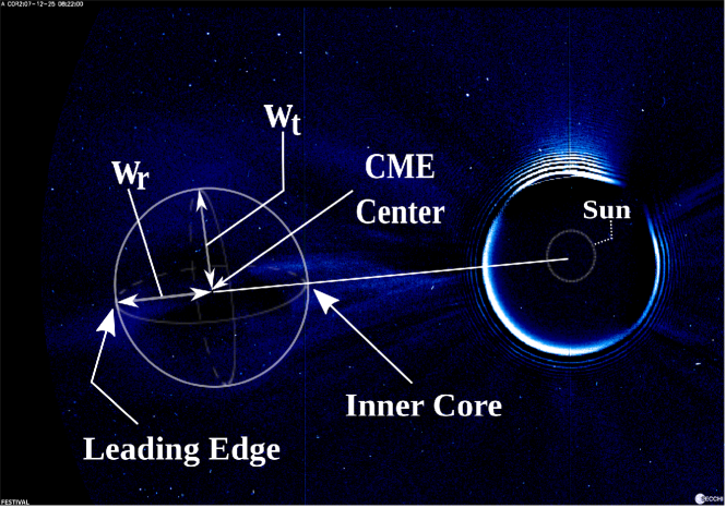
Figure 1.: A depiction of our ellipsoid model fit over an image from the second coronograph on STEREO A, taken on 25 December 2007. The two measureable halfwidths, the radial half-width ($w_{r}$), along the Sun-CME center line, and transverse halfwidth ($w_{t}$), perpendicular to the radial width in the image, are also show. A background subtraction and calibration have been applied.fig:Fig1

Using images of a CME to predict the time of arrival of in situ signatures at a location of interest has been the focus of much recent research [Davies et al. (2009), Thernisien, Vourlidas, and Howard (2009), Wood and Howard (2009), and references therein]. Wood09 modeled a CME as an inner flux-rope structure and an outer density structure created by the flux rope piling up solar wind material. In contrast, our ellipsoid model describes the outermost density structure of the CME, from the inner core to the leading edge, rather than the geometry of the inner flux rope.

Savani09 attempted to characterize the radial and transverse expansion of CMEs using a circular fit in each image. Our model adds an additional degree of freedom by independently measuring both the radial and transverse width of the CME. Wood11 found that the flux rope contained within many CMEs can be described with an elliptical cross section. As a first-order approximation, a flux rope with an elliptical cross section could be expected to drive an elliptically-curved density structure ahead of it.

To translate the elliptical cross section from the images to a 3D model, we create an ellipse of revolution around the radial axis (Figure fig:Fig1) in the same way Wood11 used an azimuthally symmetric outer density structure. This assumption is examined further in the conclusion of this paper. Another study modeled the entirety of the CME structure from the Sun to the leading edge as a “hollow croissant” [Thernisien, Vourlidas, and Howard (2009)]. Instead, our model is not anchored to the Sun but allows the forward structure of the CME to be modeled as an ellipsoid anchored to the leading edge and inner core (similar to the second model presented in Lugaz10). This means that our ellipsoid model describes the forward density structure rather than the magnetic flux-rope structure and therefore will not accurately model the conditions sunward of the inner core. By focusing on the forward structure of the CME, our model is designed to capture the three most prominent features in CME images: the leading edge, the dark cavity, and the inner core.

Our model provides a technique for tracking CMEs and predicting the arrival of in situ density signatures with an average accuracy of 2.9 hours, based on a study of three different events. Though our study is not statistical in nature, these results are quite promising and corroborate the potential role of empirical geometric models.

The paper is organized as follows. In section S-2, we introduce the data sets utilized and the methodology for creating our ellipsoid model from the imager data. Specific data and predictions for three separate CMEs are presented in section S-3. Comparisons to in situ data are described in section S-4. Discussion and conclusions are given in section S-5.

2 Instruments and Data Analysis Methodology

S-2 Our technique used the SECCHI imagers on the STEREO satellites [Howard et al. (2008)] ahead of (ST-A) and behind (ST-B) the Earth in its orbit and the LASCO imagers on the SOHO satellite [Brueckner et al. (1995), Domingo, Fleck, and Poland (1995)] at the L1 Lagrange point between the Earth and the Sun. Using images from these instruments, we tracked three CMEs out to $\approx$.3 AU and then used that data to predict the propagation and evolution of each CME out to 1 AU. In situ data from the IMPACT magnetometer [Acuna et al. (2008)] and PLASTIC [Galvin et al. (2008)] instruments on STEREO and the MFI [Lepping et al. (1995)] and 3DP [Lin et al. (1995)] instruments on the Wind spacecraft was used to assess the accuracy of our predicted arrival times.

Each of the three CMEs we studied was chosen because it transited STEREO A, STEREO B, or Wind. To make our selections, we compiled data from the STEREO and Wind in situ event lists [Jian (2010a), Jian (2010b)], thus ensuring that predictions for each chosen event could be tested with the in situ data. This selection criteria allowed us to track each CME with sets of images from either SOHO and/or STEREO and verify the predicted arrival times using STEREO or Wind. It was vital to have a set of images from two different vantage points in order to accurately determine the propagation direction of the CME in 3D space. With only one set of images, one has to make various approximations that greatly limit the accuracy of any predictions [Lugaz, Vourlidas, and Roussev (2009)]. The CMEs we selected to study crossed 1 AU on 30 December 2007 (herein referred to as “event 1”), 29 April 2008 (“event 2”), and 15 December 2008 (“event 3”).

We obtained level 0.5 images (the decompressed data in FITS format) from the STEREO and SOHO servers. FESTIVAL, an IDL-based browser designed for manipulating solar imaging data [Auch$\grave{e}$re et al. (2008)], applied a daily background subtraction and calibration to each image in order to generate the images we used, shown in Figures fig:Fig2a and fig:Fig3.

To fit the observed elliptical cross section, four measurements were acquired from each image. These measurements were $\epsilon_{LE}$ and $\epsilon_{IC}$, the elongations of the leading edge and inner core of the CME (the feature-observer-Sun angle), $\theta$, the position angle (the angle between ecliptic north and the Sun-CME center line in the image), and the transverse half-width, $w_{t}$. Figure fig:Fig2a displays the first three measurements on an image from STEREO A taken on 25 December 2007. The fourth, the transverse half-width, is shown in Figure fig:Fig3. The distance from the Sun to the observing satellite, $d_{0}$, and the propagation angle, $\phi$, (the observer-Sun-CME center angle) which will be discussed later in the paper, are also shown. Figure fig:Fig2b is a plot generated by FESTIVAL of the intensity along the cut through the image on the diagonal white line in Figure fig:Fig2a (termed “cut line”), and will herein be referred to as an “intensity profile”. The data spike near the longitude of -2.14 degrees is due to the cut line crossing over a bright star in the image. Because of the high detail of the SECCHI imagers, the intensity profile varied greatly with the location of the cut line. To reduce this variation, we modified the FESTIVAL code to plot the average intensity within $\pm$10 pixels of the cut line. This modification produced more reliable results that were less dependent upon where the cut line was drawn.

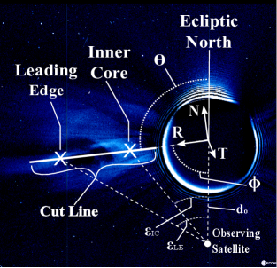
fig:Fig2a

(a) An image of a CME from STEREO A taken on 25 December 2007 (after background subtraction and calibration). The elongation of the leading edge and inner core ($\epsilon_{LE}$, $\epsilon_{IC}$), the position angle ($\theta$), the propagation angle ($\phi$), and the distance from the Sun to the observing satellite ($d_{0}$) are indicated. The modified radial, tangential, normal (RTN) coordinate system used to track the CME is also shown, centered at the Sun.

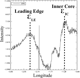
fig:Fig2b

(b) An intensity profile (plot of longitude vs. intensity) along the white cut line in Figure 2a, generated by FESTIVAL. The locations of the leading edge and inner core are indicated with dashed lines. The spike in the data near the longitude of -2.14 degrees is due to the cut line crossing over a bright start in the image. The elongation measurements are in degrees and the intensity measurements are in units of solar disk intensity (linear scale).

Figure 2.: A depiction of the characteristic variables of CME propagation (left) and a demonstration of an intensity profile (right) used to measure the elongation of the leading edge and inner core.fig:Fig2

The elongations measured from each intensity profile were converted into distance measurements using the “fixed-$\phi$” approximation [Kahler and Webb (2007)]:

$$\ilabel{eq:Eq1}r=d_{0}\frac{\sin(\epsilon)}{\sin{(\epsilon+\phi)}},$$ (1)

where is the elongation of a particular feature. Equation (1) does not account for the effects of the Thomson sphere or the possibility of a wide, 3D structure in a CME [Lugaz, Vourlidas, and Roussev (2009), Wood et al. (2011)]. Because our measurements were confined to elongations less than $16\,^{\circ}$ and radial distances less than .3 AU, the errors due to disregarding the Thomson sphere and structure of the CME are negligible [Vourlidas and Howard (2006), Howard and Tappin (2009a)]. Other approaches, such as the “harmonic mean”, have been used by other groups to translate elongations into radial distances [Lugaz, Vourlidas, and Roussev (2009)]. These techniques have proven to be better suited for specific types of CMEs, namely broad, bright CME fronts [Wood, Howard, and Socker (2010)]. To keep our approach consistent, we used the “fixed-$\phi$” method in our model for each event.

The intensity profiles in FESTIVAL measured intensity as a function of longitude (only in the horizontal direction in the image). Therefore, to properly measure the transverse width we had to rotate each image until the transverse width was completely horizontal. We then created an intensity profile across the entire width of the CME to measure its transverse size.

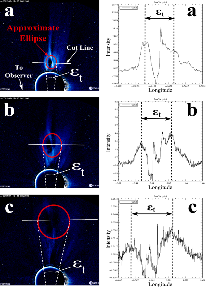
Figure 3.: Rotated images of a CME from STEREO A (left) alongside their accompanying intensity profiles (right) taken at (a) 0:22, (b) 4:22, and (c) 8:22 (HH:MM) on 25 December 2007. The intensity profiles are plots of intensity as a function of longitude (in the horizontal direction) along the white cut line shown in the images on the left. An approximate outline of the ellipse fit to each image and the elongation of the transverse width, $\epsilon_{t}$, (the angle between the lines connecting the “sides” of the CME to the observer) are overlaid on the images. The elongation of the transverse width is also indicated by the bounded arrow in the intensity profiles, with the bounds set at the center of each large density structure. The elongation measurements are in degrees and the intensity measurements are in units of solar disk intensity (linear scale).fig:Fig3

Figure fig:Fig3 displays three examples of the rotated CME images from STEREO A (left) alongside their accompanying intensity profiles (right) taken at (a) 00:22, (b) 04:22, and (c) 08:22 (HH:MM UT) on 25 December 2007. An approximate outline of the ellipse we fit to each image and the elongation of the transverse width are overlaid on the images. The elongation of the transverse width (the angle between the two lines connecting the “sides” of the CME to the observing satellite) is also indicated by the bounded arrow in the intensity profiles. The intensity profile in Figure fig:Fig3a shows how the determination of the $\epsilon_{t}$ can be ambiguous when using a single image. To determine the appropriate features to use in measuring $\epsilon_{t}$, a sequence of images was examined and features that remained bright over a large range of elongations were selected. The bounds on the transverse elongation (the dotted lines in the right panels of Figure fig:Fig3) were set at the middle of the large density enhancements in the intensity profiles. The transverse elongation was converted to a distance measurement using

$$\ilabel{eq:Eq2}w_{t}=d_{0}\frac{\sin(\phi)}{\sin{(\phi+\epsilon_{c})}}\tan{\left(\frac{\epsilon_{t}}{2}\right)},$$ (2)

where $\epsilon_{c}$ is the elongation of the CME center and $w_{t}$ is the transverse half-width of the CME. Equation (2) is derived in the appendix.

FESTIVAL was used to calculate the position angle, $\theta$, of the CME in each frame by measuring the location of the CME center with respect to the Sun. However, the position angle was slightly different from the latitudinal angle, $\theta^{\prime}$, (the angle between ecliptic north and the Sun-CME center line in 3D space). Projection effects had to be considered to correctly determine the trajectory of the CME. Equation (3) is derived in the appendix and gives the latitudinal angle by

$$\ilabel{eq:Eq3}\theta^{\prime}=\arcsin{\left(\sqrt{\sin^{2}(\theta)\sin^{2}(\phi)+\cos^{2}(\phi)}\right)}.$$ (3)

To determine the propagation angle, $\phi$, of each CME, we compared near-simultaneous images, taken less than ten minutes apart, from the two observing satellites. Assuming that the features measured in both sets of images were the same, the radial distances associated with both satellite elongation data sets should be equal, even though the respective elongation values were different. We compared the inner core data sets from both observing satellites (between 15-30 data points for the events in our study) and determined the value for $\phi$ which resulted in the smallest sum of the absolute errors between the radial distances in both data sets. We then compared the leading edge data sets from both observing satellites in a similar manner to determine a second value for $\phi$. We then used the average of both $\phi$ values to obtain a final propagation angle for each event. In other words, the selected value for $\phi$ was the one that resulted in the least error between the leading edge and inner core data sets for both observing satellites.

Our methodology can be summarized as follows:

1. Measure the variables which characterize the propagation and expansion of the CME ($w_{r}$, $w_{t}$, $r_{c}$, $\theta$, and $\phi$) using the density structures seen in the imager data.

2. Generate a mathematical 3D ellipsoid surface (as a function of time) using the measured variables in step 1 (see Equation 5).

3. Calculate the predicted arrival times in the in situ data using the time-dependent mathematical ellipsoid.

3 Using Imager Data to Generate Predictions

S-3

Using the methodology described above, we now examine the propagation of three events. The center of each CME was calculated as the mean of the leading edge and inner core radial positions. A line was fit to the data set for the center of each event to predict its location beyond the distance of the image data. For event 2, a straight line was fit to the data after about 19:00 on April 26th, because its inner core experienced a brief acceleration at that point in time. A straight line was fit to the entire data set from event 3. Event 1 exhibited a slow initial velocity ($\leq$100 km/s) and gradually “ballooned” off the surface of the Sun. This initial behavior typically leads to extended, slow acceleration [Sheeley et al. (1999)] and required a different fitting technique because it did not propagate with constant speed. Although its acceleration decreased within the radial distance over which images were obtained, it was still significant enough to strongly affect the estimated arrival time; a linear fit of the last 15 data points produced an arrival time that was nearly 24 hours late when compared with the in situ data. Following the example of Sheeley99, we fit

$$\ilabel{eq:Eq4}R(t)=r_{0}+2r_{a}\ln{\left[\cosh{\left(\frac{v_{a}(t+\Delta t_{0})}{2r_{a}}\right)}\right]}$$ (4)

to the data series for event 1, in which $R(t)$ is the radial distance of the feature as a function of time, $r_{0}$ is radial position at $t=-\Delta t_{0}$, $v_{a}$ is the asymptotic velocity, and $r_{a}$ is the e-folding distance at which the asymptotic velocity is approached. Instead of measuring these values independently, we optimized $r_{a}$, $r_{0}$, and $v_{a}$ in order to achieve a quality fit.

Table tab:Tab1 displays the variables which characterize the trajectory of the CME. The columns, from left to right, list the propagation angle (the observer-Sun-CME center angle), the latitudinal angle (between ecliptic north and the Sun-CME center line), the asymptotic velocity, and the e-folding distance at which the asymptotic velocity is approached. For events 2 and 3, the asymptotic velocity was taken as the velocity from the linear fit of the data. Note: The latitudinal angle ($\theta^{\prime}$) of Event 2 changed as it propagated away from the Sun (see Figure fig:Fig6). The value listed in Table tab:Tab1 is the latitudinal angle at the time it crossed 1 AU.

Figure fig:Fig4 displays the radial distance of the leading edge (LE) and inner core (IC) as a function of time for each event, also known as a height-time diagram [Sheeley et al. (1999)]. Additionally, the center of each event, along with the respective fit line, is plotted. The data obtained from the SOHO and STEREO images, displayed in different colors, demonstrates the good agreement between both data sets.

Table 1.: The variables associated with the kinematics of the three CMEs in our study. $v_{a}$ is the asymptotic velocity of the CME center, $r_{a}$ is the e-folding distance at which the asymptotic velocity is approached, $\phi$ is the observer-Sun-CME center angle (from STEREO A), and $\theta^{\prime}$ is the angle between ecliptic north and the Sun-CME center line.tab:Tab1

Event	$\phi$ (degrees)	$\theta^{\prime}$ (degrees)	$v_{a}$ (km/s)	$r_{a}$ (AU)
1	58.15	93.64	308.85	.068
2	61.70	85.10	584.42	n/a
3	41.40	84.94	578.89	n/a

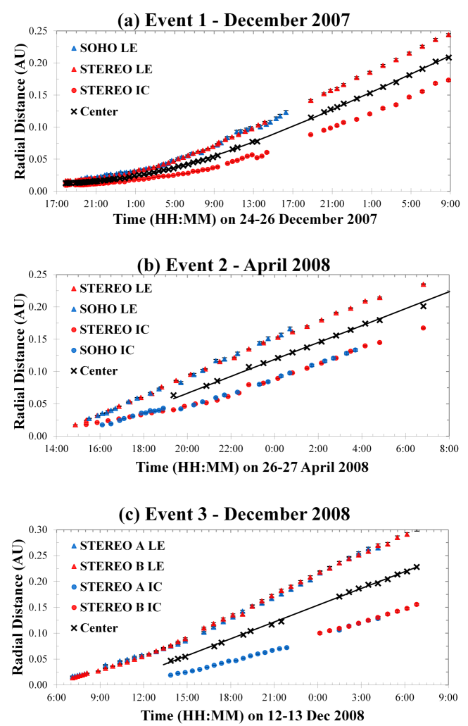
Figure 4.: A height-time diagram (plot of radial distance vs. time) for the leading edge and inner core of the CME for events 1 (a), 2 (b), and 3 (c). The CME center and the respective fit line for each event are also plotted. Where not visible, the error bars on each data point are approximately the size of the marker.fig:Fig4

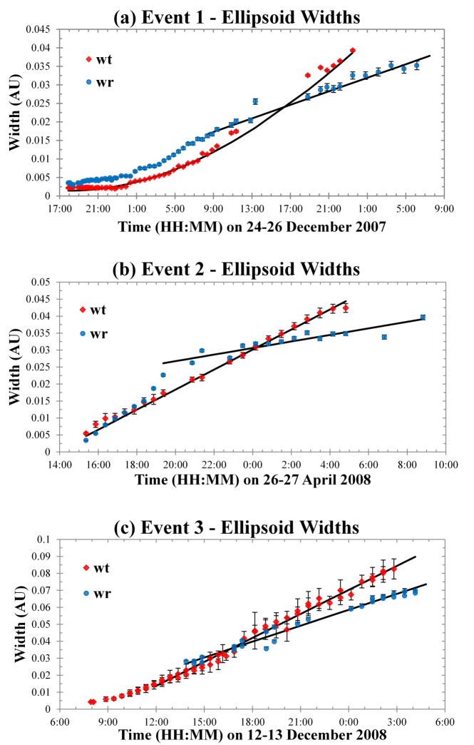
Figure 5.: A plot of the radial CME half-width along the Sun-CME center line ($w_{r}$) and the transverse half-width ($w_{t}$) of the ellipse fit to each image for events 1 (a), 2 (b), and 3(c). The trend lines used to predict the growth of both half-widths are also shown. Where not visible, the error bars on each data point are approximately the size of the marker.fig:Fig5

The radial half-width of the ellipsoid, $w_{r}$, was calculated by taking half the distance between the leading edge and inner core. Figure fig:Fig5 displays the growth of the radial half-width and the transverse half-width, $w_{t}$, for each event, as well as respective fit used on each data set.

It was necessary to study the position angle ($\theta$) as a function of time for each CME. As events 1 and 3 propagated outwards, $\theta$ remained relatively constant with small fluctuations about the average, attributable to the user-related error introduced by our technique. In contrast, the position angle for event 2 was initially $\approx 70\,^{\circ}$ and then increased significantly. To describe this trend, we performed a least squares fit with an arctangent function, as shown in Figure fig:Fig6. This trend-line fit the data quite well and indicated that event 2 did not propagate along a purely radial trajectory.

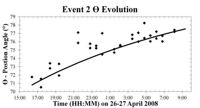
Figure 6.: The evolution of the position angle ($\theta$) for event 2 as it propagated away from the Sun. The accompanying trend line was generated by a least squares fit of an arctangent function. The effectiveness of this fit inidicates that event 2 did not propagation in a purely radial direction.fig:Fig6

To determine the arrival time for each event in our study, we defined a modified radial, tangential, normal (RTN) coordinate system, with the R-axis pointing from the Sun center to the CME center, the N-axis being perpendicular to the R-axis and in the same plane as the ecliptic north, and the T-axis completing the orthogonal coordinate system (Figure fig:Fig2a). In other words, our coordinate system was defined using the propagation angle ($\phi$) and the latitudinal angle ($\theta^{\prime}$) and was designed such that each width used to define our ellipsoid was directed along an axis. Then, using the time-dependent location of the CME center ($r_{c}$) and its radial, transverse, and normal half-widths ($w_{r}$, $w_{t}$, and $w_{n}$), we mathematically modeled the 3D surface of the ellipsoid. This surface is shown in Figure fig:Fig1 and is defined as

$$\ilabel{eq:Eq5}\left(\frac{r-r_{c}}{w_{r}(t)}\right)^{2}+\left(\frac{t}{w_{t}(t)}\right)^{2}+\left(\frac{n}{w_{n}(t)}\right)^{2}=1,$$ (5)

in which ($r$, $t$, $n$) are the coordinates of the surface. As previously stated, we assumed that the transverse half-width was equal to the normal half-width ($w_{t}$ = $w_{n}$). This assumption is examined in detail in the conclusion. Using the position of the transited satellite and the equation describing the time-dependent surface of the ellipsoid in the new RTN coordinate system, we calculated when the leading and trailing edge of the ellipsoid would traverse the satellite. These two arrival times were compared to the in situ data from the transited satellite.

4 Comparisons to In Situ Data

S-4

Coronal mass ejections are characterized by a variety of in situ signatures including changes in the density, the magnitude and direction of the magnetic field, and the velocity of the solar wind [Jian et al. (2006), and references therein]. Figures fig:Fig7, fig:Fig8, and fig:Fig9 display the in situ data for each event over-plotted with our predicted arrival times. The arrows in each density plot identify the density enhancements we compared to our ellipsoid model. We chose to compare our model to the first density enhancement and the enhancement directly following the low-density cavity. The first density enhancement was selected because the ellipsoid model was fit to the leading edge, which could reasonably be expected to cross the in situ observer first. The enhancement following the low-density cavity was chosen because the ellipsoid was also fit through the inner core, which directly followed the dark, low-density cavity in the images. Figure fig:Fig7 shows that multiple density enhancements occurred after the feature to which we compared our predictions. This highlights the fact that the predictions from the ellipsoid model do not accurately describe density enhancements sunward of the inner core, as stated in the introduction of this paper.

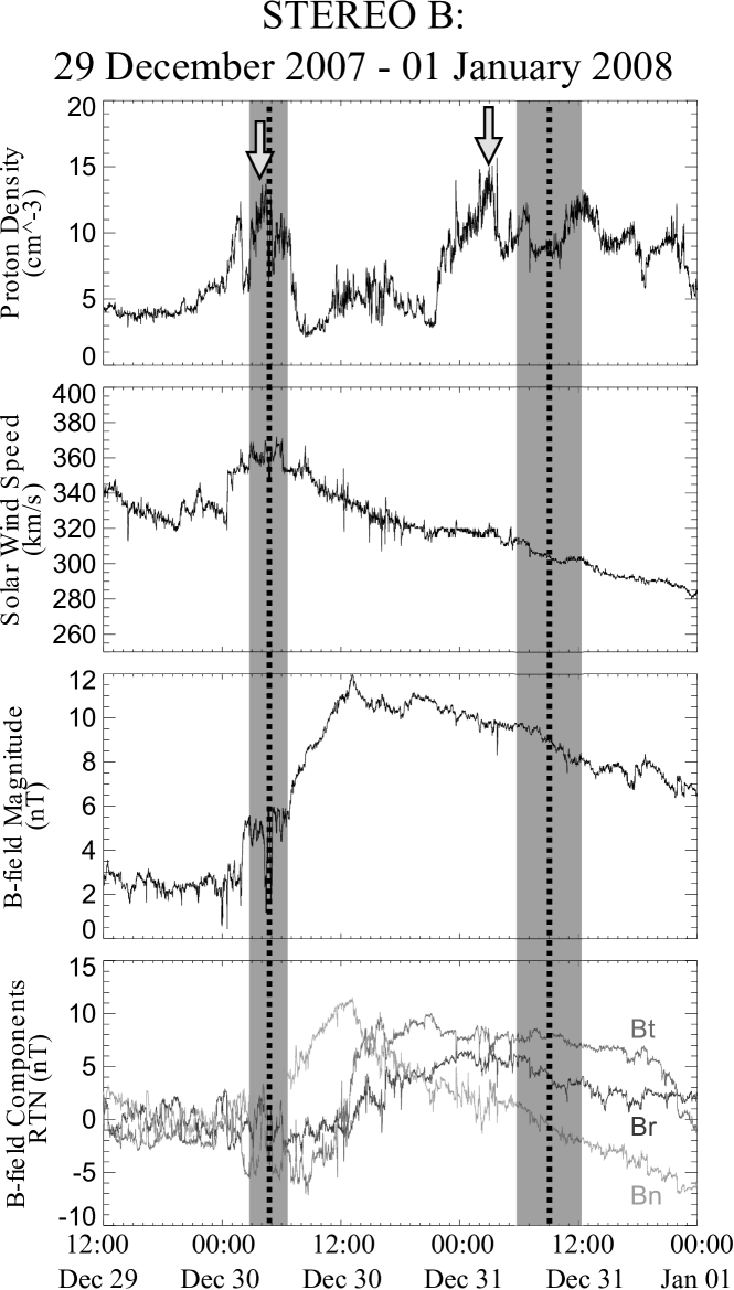
Figure 7.: Event 1 in the in situ data from 30 December 2007 to 01 January 2008, as observed by STEREO B when it was about $23\,^{\circ}$ off the Sun-Earth line. The panels, from top to bottom, display the proton density, solar wind speed, magnitude of the magnetic field and the components of the magnetic field in an RTN coordinate system. The predicted arrival times from our ellipsoid model are marked by the dotted black lines and bounded by $\pm 1\sigma$ (grey). The arrows overlaid on the density plot mark the enhancements we compared to our model, namely the first enhancement and the one directly following the low-density cavity.fig:Fig7

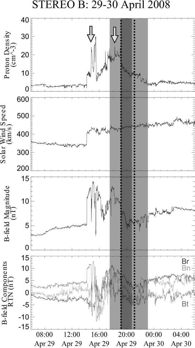
Figure 8.: Event 2 in the in situ data from 29 April 2008 to 30 April 2008, as observed by STEREO B when it was about $24\,^{\circ}$ off the Sun-Earth line. The panels, from top to bottom, display the proton density, solar wind speed, magnitude of the magnetic field and the components of the magnetic field in an RTN coordinate system. The predicted arrival times from our ellipsoid model are marked by the dotted black lines and bounded by $\pm 1\sigma$ grey/black boxed). The $\pm 1\sigma$ bounds overlap and are shaded darker in the overlapping region. The arrows overlaid on the density plot mark the enhancements we compared to our model, namely the first enhancement and the one directly following the low-density cavity.fig:Fig8

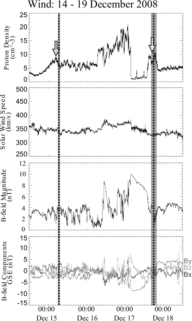
Figure 9.: Event 3 in the in situ data from 14 December 2008 to 19 December 2008, as observed by Wind when it was roughly 1.5 million kilometers upstream of the Earth. The panels, from top to bottom, display the proton density, solar wind speed, magnitude of the magnetic field and the components of the magnetic field in an RTN coordinate system. The predicted arrival times from our ellipsoid model are marked by the dotted black lines and bounded by $\pm 1\sigma$ (grey). The arrows overlaid on the density plot mark the enhancements we compared to our model, namely the first enhancement and the one directly following the low-density cavity. Though this is preliminary browse data, it agrees well with similar data from the Advanced Composition Explorer (ACE).fig:Fig9

Table tab:Tab2 displays the comparison between the predictions generated by our model and the density enhancements in the in situ data. The columns, from left to right, identify the event number and transited satellite, the predicted time of the beginning/end of the model transit, the time of the density enhancement in the in situ data, and difference between the predicted and observed arrival time (in hours and standard deviations). The uncertainty for the in situ time was calculated as half the temporal width of the density enhancement.

Table 2.: The predicted beginning and end of the ellipsoid’s transit compared to the first density enhancement and the one directly following the low-density cavity in the in situ data, respectively. The transited satellite and event number are recorded in the left-hand column for three coronal mass ejections.tab:Tab2

Event/satellite	Predicted Arrival Time	In Situ Arrival Time	Hours Away	$\sigma$ Away
1	12/30/07 4:56 $\pm$ 2:07	12/30/07 4:00 $\pm$ 3:00	0.95	0.26
ST-B	12/31/07 9:09 $\pm$ 3:17	12/31/07 3:00 $\pm$ 0:45	6.16	1.83
2	4/29/08 19:12 $\pm$ 1:38	4/29/08 14:45 $\pm$ 0:45	4.46	2.47
ST-B	4/29/08 21:08 $\pm$ 2:05	4/29/08 18:15 $\pm$ 1:00	2.90	1.25
3	12/15/08 6:45 $\pm$ 0:20	12/15/08 4:30 $\pm$ 3:00	2.26	0.75
Wind	12/17/08 17:41 $\pm$ 1:08	12/17/08 17:15 $\pm$ 3:00	0.44	0.14

To further test our model, we compared the temporal separation of the density peaks tabulated in Table tab:Tab2. Table tab:Tab3 displays the predicted temporal separation to that seen in the in situ data. The far right column displays the difference between the predicted duration from the model and the duration in the in situ data. The average accuracy of these predictions was 2.6 hours.

Table 3.: The predicted temporal duration of each CME compared with the temporal separation seen in the in situ data, defined as the time between the first density enhancement and the one following the low-density cavity.tab:Tab3

Event	Ellipsoid Width (hours)	In situ Width (hours)	Error
1	28.22$\pm$3.91	23.00	5.22
2	1.94$\pm$2.67	3.50	-1.56
3	58.93$\pm$1.19	60.75	-1.82

5 Summary and Conlusions

S-5

Although tracking and predicting the propagation of coronal mass ejections using images is nothing new, our study introduces two tools that could prove useful in the future study of CMEs. First, we demonstrate the use of intensity profiles in FESTIVAL (Figures fig:Fig2b and fig:Fig3) as an alternative way to construct height-time diagrams and study the transverse growth of CMEs. Previous methods using image profiles have been constrained to constant position angles [Sheeley et al. (2008)]. The intensity profiles implemented in FESTIVAL are not constrained in this manner and can therefore track CMEs with varying position angles (such as seen in event 2). Additionally, intensity profiles provide a method for determining the uncertainty on each measurement (see Figure fig:Fig2b), instead of assuming a certain percent error in each measurement based on the imager used [Wood and Howard (2009), Lugaz et al. (2010), Wood, Howard, and Socker (2010)].

Second, we introduce our ellipsoid model and test it on three separate CMEs. The results suggest that the ellipsoid model may prove useful in tracking and predicting the expansion and trajectory of CMEs. Our predictions were an average of 2.9 hours away from the arrival of particular density enhancements in the in situ data for the three events. The average of the uncertainty in our predicted arrival times was 1.9 hours and compares well with previous work [Davis et al. (2009), see their Table 2]. Howard09b and Wood11 used synthetic images obtained from their 3D CME density models to track the kinematics of CMEs and, when compared to the in situ data, achieved ideal accuracies of 3.5 hours and less than an hour, respectively. Lugaz10 used a model that accounted for the 3D structure of CMEs and obtained an accuracy of 11 hours. Using the synthetic image technique, Wood09 predicted the in situ signatures of the April 2008 CME (our event 2) with accuracies ranging from 1.5 to 10 hours. Though our ellipsoid model is as accurate as these previous studies, this not an entirely appropriate comparison. The aforementioned models incorporated measurements from the Sun to 1 AU, except Lugaz10, who used data out to elongations of about $45\,^{\circ}$. The fact that our predictions were obtained using data closer to the Sun (measurements below .3 AU and elongations less than $16\,^{\circ}$) and attained a similar accuracy is a promising result. Our ellipsoid model demonstrates the possible potential of being able to accurately predict CME effects when the CME is still days away from reaching 1 AU.

Some of the errors given in Tables tab:Tab2 and tab:Tab3 can be attributed to our neglect of the effects of the Thomson sphere and the 3D structure of the CME. Another plausible source of error originates from using an ellipse of revolution around the radial axis, making our model azimuthally symmetric. This meant that the third width of our ellipsoid model (approximately along the imager’s line-of-sight) was set equal to the transverse width. The use of an azimuthally symmetric structure (an ellipse of revolution) is not intended to represent an accurate physical assumption, but rather arises from the limitations of the two vantage points used in our study. To circumvent this, one could examine images from the transited satellite to measure this third width. Additionally, the fact that all of the predictions of our model were later than the actual in situ times may prove useful in understanding the physics of CME propagation between .3 and 1 AU.

The study of three CMEs also shed light on a few assumptions made in some current approaches. Past studies have often assumed that CMEs travel with c onstant velocity throughout the HI-1 field of view [Davis et al. (2009), Savani et al. (2009), Liu et al. (2010)], which begins at an elongation of $4\,^{\circ}$, or $\approx$.07 AU for the events in our study. Event 1 exhibited significant acceleration beyond an elongation of $14\,^{\circ}$, demonstrating that this assumption does not hold true for all CMEs. Savani09used a circular cross section to model the flux rope geometry. Figure fig:Fig5 shows that the circular cross section assumption is roughly true close to the Sun, but as the CME propagates away from the Sun, the two radii observed in the images become significantly different. Additionally, an examination of the transverse, or normal, growth of events 1 and 2 (Figure fig:Fig5) showed that the assumption of self-similar expansion does not hold true for all CMEs. Though many CMEs certainly exhibit self-similar expansion, our results indicate that this assumption can be made only after a careful examination of the data.

CMEs are a diverse group of structures in the solar wind and require a flexible tool to adequately track and predict their propagation. Their radial velocity and transverse growth can accelerate beyond .25 AU (event 1), their expansion rates can drastically change (event 2) as far out as .08 AU, and their direction of propagation can change over time (event 2). Our ellipsoid model provides a method to incorporate this variety using a small number of parameters. After examining three CMEs using the ellipsoid model, we find it capable of accurately predicting the occurrence of density enhancements and the duration of an event in the density data. Though this is not a statistical study, the results show some promise that the forward structure of a CME, from the inner core to the leading edge, can be effectively modeled as an ellipsoid.

6 Acknowledgements

S-Ack

STEREO/HI was developed by a consortium comprising RAL, the University of Birmingham (UK), CSL (Belgium) and NRL (USA). SECCHI, led by NRL, involves additional collaborators from LMSAL, GSFC (USA), MPI (Germany), IOTA and IAS (France). We thank the PIs of the STEREO, SOHO and Wind instruments utilized herein: R. A. Howard, G. Brueckner, J. Luhmann, M. Acuna, A. Galvin, R. Lin and R. Lepping. We would like to thank Elie Soubri$\grave{e}$ and Fr$\acute{e}$d$\acute{e}$ric Auch$\grave{e}$re of the Institut d’Astrophysique Spatiale (IAS) for assisting with the modifications of FESTIVAL’s code. We thank Dr. Aaron Breneman for reviewing the paper, Dr. Dan Cronin-Hennessy for his insightful conversations concerning the propagation of uncertainties, and Ying Liu for feedback regarding our methods.

This research was supported through a grant from the University of Minnesota Undergraduate Research Program and by NASA grant NNX09AG82G.

Appendix: Deriving Equations (2) and (3)

Equation 2 is derived from the geometry presented in Figure fig:FigA1, in which $w_{t}$ is half the transverse distance width of the CME, $\epsilon_{t}$ is the elongation of the transverse width of the CME, $\epsilon_{c}$ is the elongation of the CME center, $d_{0}$ is the distance from the observer to the Sun, $R_{O-CME}$ is the distance from the observer to the CME center, and $\phi$ is the propagation angle (the observer-Sun-CME center angle).

Figure 10.: The geometry of an arbitrary CME propagation with the ellipsoid cross section shown. The method for converting the elongation width of the CME ($\epsilon_{t}$) to the distance half-width of the CME ($w_{t}$) is displayed. Also shown is the elongation of the CME center ($\epsilon_{c}$), the distance from the observer to the Sun ($d_{0}$), the distance from the observer to the CME center ($R_{O-CME}$), and the propagation angle ($\phi$).fig:FigA1

Using the sine law on the triangle connecting the Sun, observer, and CME center yields

$$\sin{(\phi)}d_{0}=\sin{(180-\phi-\epsilon_{c})}R_{O-CME}.$$ (A1)

Applying the right triangle rule to the triangle connecting the CME center, observer, and CME side results in

$$\tan{\left(\frac{\epsilon_{t}}{2}\right)}=\frac{w_{t}}{R_{O-CME}}.$$ (A2)

Combining (A1) and (A2) produces Equation (2)

$$w_{t}=R_{0}\frac{\sin{(\phi)}}{\sin{(\phi+\epsilon_{c})}}\tan{\left(\frac{\epsilon_{t}}{2}\right)}.$$ (A3)

Equation 3 is derived from the geometry presented in Figure fig:FigA2, in which the “Plane of the Image” is an arbitrary plane onto which all features are projected to form the image seen by the observing satellite. $\theta^{\prime}$ is the latitudinal angle, $\theta$ is the position angle seen in the image, $\epsilon_{c}$ is the elongation of the CME center, $\phi$ is the propagation angle, and $d_{0}$ is the distance from the observer to the Sun.

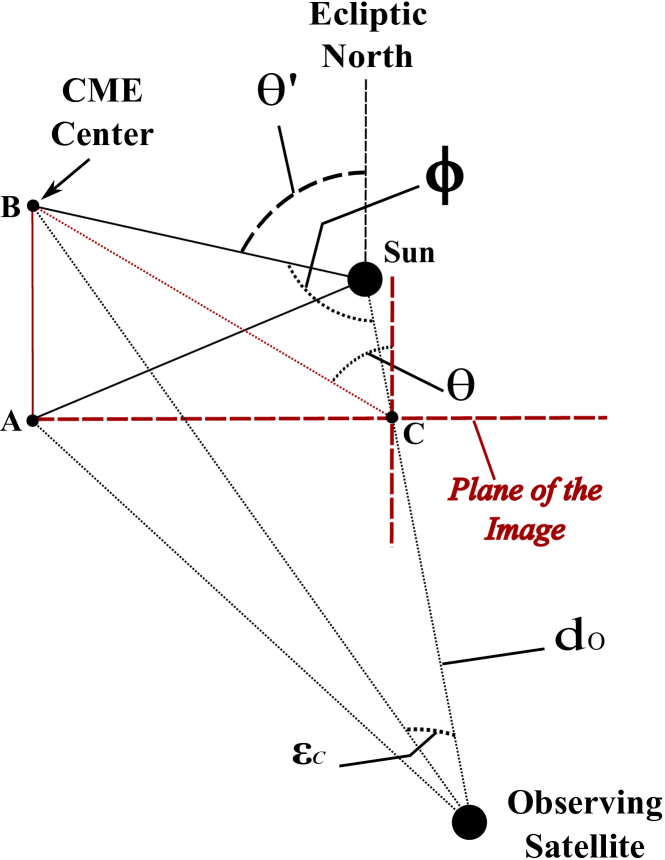
Figure 11.: The geometry of an arbitrary CME propagation. The relationship between the position angle ($\theta$) as viewed from the image and the latitudinal angle ($\theta^{\prime}$) in 3D space is displayed. Also shown is the elongation of the CME center ($\epsilon_{c}$), the propagation angle ($\phi$), and the plane onto which all features are projected to form the image seen by the observing satellite (“Plane of the Image”).fig:FigA2

Applying the right triangle rule to the triangle connecting A, B, and the Sun (S) yields (“AS” is the length of the line connecting A and the Sun)

$$\sin{(\theta^{\prime})}=\frac{AS}{BS}.$$ (A4)

Defining $\phi^{\prime}$ as the A-Sun-C angle, we apply the right triangle rule to ABC and to BCS to get

$$\sin(\theta)=\frac{AC}{BC}=\frac{AS\sin{(\phi^{\prime})}}{BS\sin(\phi)}.$$ (A5)

$\phi^{\prime}$ can be expressed in terms of $\phi$ and $\theta^{\prime}$:

$$\phi^{\prime}=\arccos\left(\frac{\cos(\phi)}{\sin{(\theta^{\prime})}}\right).$$ (A6)

We use the right triangle rule to define from (A6) and then combine it with (A4) and (A5) to get

$$\sin{(\theta^{\prime})}=\frac{\sin(\theta)\sin(\phi)}{\sqrt{1-\frac{\cos^{2}(\phi)}{\sin^{2}{(\theta^{\prime})}}}}.$$ (A7)

Multiplying both sides by the quantity in the square-root and then squaring both sides yields

$$\sin^{2}(\theta^{\prime})-\cos^{2}(\phi)=\sin^{2}(\theta)\sin^{2}(\phi).$$ (A8)

Solving for we obtain the final expression, Equation (3):

$$\theta^{\prime}=\arcsin{\left(\sqrt{\sin^{2}(\theta)\sin^{2}(\phi)+\cos^{2}(\phi)}\right)}.$$ (A9)

References

- Acuna et al. (2008) Acuna, M.H., Curtis, D., Scheifele, J.L., Russell, C.T., Schroeder, P., Szabo, A., Luhmann, J.G.: 2008, The stereo/impact magnetic field experiment. Space Science Reviews 136(1-4), 203 – 226.
- Auchre et al. (2008) Auchre, F., Soubri, E., Bocchialini, K., LeGall, F.: 2008, Festival: A multiscale visualization tool for solar imaging data. Solar Physics 248(2), 213 – 224.
- Brueckner et al. (1995) Brueckner, G.E., Howard, R.A., Koomen, M.J., Korendyke, C.M., Michels, D.J., Moses, J.D., Socker, D.G., Dere, K.P., Lamy, P.L., Llebaria, A., Bout, M.V., Schwenn, R., Simnett, G.M., Bedford, D.K., Eyles, C.J.: 1995, The large angle spectroscopic coronagraph (lasco). Solar Physics 162(1-2), 357 – 402.
- Davies et al. (2009) Davies, J.A., Harrison, R.A., Rouillard, A.P., Sheeley, N.R., Perry, C.H., Bewsher, D., Davis, C.J., Eyles, C.J., Crothers, S.R., Brown, D.S.: 2009, A synoptic view of solar transient evolution in the inner heliosphere using the heliospheric imagers on stereo. Geophysical Research Letters 36.
- Davis et al. (2009) Davis, C.J., Davies, J.A., Lockwood, M., Rouillard, A.P., Eyles, C.J., Harrison, R.A.: 2009, Stereoscopic imaging of an earth-impacting solar coronal mass ejection: A major milestone for the stereo mission. Geophysical Research Letters 36.
- Domingo, Fleck, and Poland (1995) Domingo, V., Fleck, B., Poland, A.I.: 1995, The soho mission: An overview. Solar Physics 162(1-2), 1 – 37.
- Galvin et al. (2008) Galvin, A.B., Kistler, L.M., Popecki, M.A., Farrugia, C.J., Simunac, K.D.C., Ellis, L., Mobius, E., Lee, M.A., Boehm, M., Carroll, J., Crawshaw, A., Conti, M., Demaine, P., Ellis, S., Gaidos, J.A., Googins, J., Granoff, M., Gustafson, A., Heirtzler, D., King, B., Knauss, U., Levasseur, J., Longworth, S., Singer, K., Turco, S., Vachon, P., Vosbury, M., Widholm, M., Blush, L.M., Karrer, R., Bochsler, P., Daoudi, H., Etter, A., Fischer, J., Jost, J., Opitz, A., Sigrist, M., Wurz, P., Klecker, B., Ertl, M., Seidenschwang, E., Wimmer-Schweingruber, R.F., Koeten, M., Thompson, B., Steinfeld, D.: 2008, The plasma and suprathermal ion composition (plastic) investigation on the stereo observatories. Space Science Reviews 136(1-4), 437 – 486.
- Howard et al. (2008) Howard, R.A., Moses, J.D., Vourlidas, A., Newmark, J.S., Socker, D.G., Plunkett, S.P., Korendyke, C.M., Cook, J.W., Hurley, A., Davila, J.M., Thompson, W.T., St Cyr, O.C., Mentzell, E., Mehalick, K., Lemen, J.R., Wuelser, J.P., Duncan, D.W., Tarbell, T.D., Wolfson, C.J., Moore, A., Harrison, R.A., Waltham, N.R., Lang, J., Davis, C.J., Eyles, C.J., Mapson-Menard, H., Simnett, G.M., Halain, J.P., Defise, J.M., Mazy, E., Rochus, P., Mercier, R., Ravet, M.F., Delmotte, F., Auchere, F., Delaboudiniere, J.P., Bothmer, V., Deutsch, W., Wang, D., Rich, N., Cooper, S., Stephens, V., Maahs, G., Baugh, R., McMullin, D., Carter, T.: 2008, Sun earth connection coronal and heliospheric investigation (secchi). Space Science Reviews 136(1-4), 67 – 115.
- Howard and Tappin (2009a) Howard, T.A., Tappin, S.J.: 2009a, Interplanetary coronal mass ejections observed in the heliosphere: 1. review of theory. Space Science Reviews 147(1-2), 31 – 54.
- Howard and Tappin (2009b) Howard, T.A., Tappin, S.J.: 2009b, Interplanetary coronal mass ejections observed in the heliosphere: 3. physical implications. Space Science Reviews 147(1-2), 89 – 110.
- Hundhausen et al. (1984) Hundhausen, A.J., Sawyer, C.B., House, L., Illing, R.M.E., Wagner, W.J.: 1984, Coronal mass ejections observed during the solar maximum mission - latitude distribution and rate of occurrence. Journal of Geophysical Research-Space Physics 89(NA5), 2639 – 2646.
- Illing and Hundhausen (1986) Illing, R.M.E., Hundhausen, A.J.: 1986, Disruption of a coronal streamer by an eruptive prominence and coronal mass ejection. Journal of Geophysical Research-Space Physics 91(A10), 951 – 960.
- Jian et al. (2006) Jian, L., Russell, C.T., Luhmann, J.G., Skoug, R.M.: 2006, Properties of interplanetary coronal mass ejections at one au during 1995-2004. Solar Physics 239(1-2), 393 – 436.
- Jian (2010a) Jian, L.: 2010a, Interplanetary coronal mass ejections (icmes) from wind and ace data during 1995-2009, http://www-ssc.igpp.ucla.edu/~jlan/ACE/Level3/ICME˙List˙from˙Lan˙Jian.pdf%.
- Jian (2010b) Jian, L.: 2010b, List of interplanetary coronal mass ejections (icmes) observed by stereo a/b., http://www-spc.igpp.ucla.edu/~jlan/STEREO/Level3/STEREO˙Level3˙ICME.pdf.
- Kahler and Webb (2007) Kahler, S.W., Webb, D.F.: 2007, V arc interplanetary coronal mass ejections observed with the solar mass ejection imager. Journal of Geophysical Research-Space Physics 112(A9).
- Lepping et al. (1995) Lepping, R.P., Acuna, M.H., Burlaga, L.F., Farrell, W.M., Slavin, J.A., Schatten, K.H., Mariani, F., Ness, N.F., Neubauer, F.M., Whang, Y.C., Byrnes, J.B., Kennon, R.S., Panetta, P.V., Scheifele, J., Worley, E.M.: 1995, The wind magnetic-field investigation. Space Science Reviews 71(1-4), 207 – 229.
- Lin et al. (1995) Lin, R.P., Anderson, K.A., Ashford, S., Carlson, C., Curtis, D., Ergun, R., Larson, D., McFadden, J., McCarthy, M., Parks, G.K., Reme, H., Bosqued, J.M., Coutelier, J., Cotin, F., Duston, C., Wenzel, K.P., Sanderson, T.R., Henrion, J., Ronnet, J.C., Paschmann, G.: 1995, A 3-dimensional plasma and energetic particle investigation for the wind spacecraft. Space Science Reviews 71(1-4), 125 – 153.
- Liu et al. (2010) Liu, Y., Davies, J.A., Luhmann, J.G., Vourlidas, A., Bale, S.D., Lin, R.P.: 2010, Geometric triangulation of imaging observations to track coronal mass ejections continuously out to 1 au. Astrophysical Journal Letters 710(1), L82 – L87.
- Lugaz, Vourlidas, and Roussev (2009) Lugaz, N., Vourlidas, A., Roussev, I.: 2009, Deriving the radial distances of wide coronal mass ejections from elongation measurements in the heliosphere - application to cme-cme interaction. Annales Geophysicae 27(9), 3479 – 3488.
- Lugaz et al. (2008) Lugaz, N., Vourlidas, A., Roussev, I., Jacobs, C., Manchester, W.B., Cohen, O.: 2008, The brightness of density structures at large solar elongation angles: What is being observed by stereo secchi? Astrophysical Journal Letters 684(2), L111 – L114.
- Lugaz et al. (2010) Lugaz, N., Hernandez-Charpak, J.N., Roussev, I., Davis, C.J., Vourlidas, A., Davies, J.A.: 2010, Determining the azimuthal properties of coronal mass ejections from multi-spacecraft remote-sensing observations with stereo secchi. Astrophysical Journal 715(1), 493 – 499.
- Savani et al. (2009) Savani, N.P., Rouillard, A.P., Davies, J.A., Owens, M.J., Forsyth, R.J., Davis, C.J., Harrison, R.A.: 2009, The radial width of a coronal mass ejection between 0.1 and 0.4 au estimated from the heliospheric imager on stereo. Annales Geophysicae 27(11), 4349 – 4358.
- Schwenn (1996) Schwenn, R.: 1996, An essay on terminology, myths, and known facts: Solar transient, flare, cme, driver gas, piston, bde, magnetic cloud, shock wave, geomagnetic storm. Astrophysics and Space Science 243(1), 187 – 193.
- Sheeley et al. (1999) Sheeley, N.R., Walters, J.H., Wang, Y.M., Howard, R.A.: 1999, Continuous tracking of coronal outflows: Two kinds of coronal mass ejections. Journal of Geophysical Research-Space Physics 104(A11), 24739 – 24767.
- Sheeley et al. (2008) Sheeley, N.R., Herbst, A.D., Palatchi, C.A., Wang, Y.M., Howard, R.A., Moses, J.D., Vourlidas, A., Newmark, J.S., Socker, D.G., Plunkett, S.P., Korendyke, C.M., Burlaga, L.F., Davila, J.M., Thompson, W.T., St Cyr, O.C., Harrison, R.A., Davis, C.J., Eyles, C.J., Halain, J.P., Wang, D., Rich, N.B., Battams, K., Esfandiari, E., Stenborg, G.: 2008, Heliospheric images of the solar wind at earth. Astrophysical Journal 675(1), 853 – 862.
- Thernisien, Vourlidas, and Howard (2009) Thernisien, A., Vourlidas, A., Howard, R.A.: 2009, Forward modeling of coronal mass ejections using stereo/secchi data. Solar Physics 256(1-2), 111 – 130.
- Vourlidas and Howard (2006) Vourlidas, A., Howard, R.A.: 2006, The proper treatment of coronal mass ejection brightness: A new methodology and implications for observations. Astrophysical Journal 642(2), 1216 – 1221.
- Wood and Howard (2009) Wood, B.E., Howard, R.A.: 2009, An empirical reconstruction of the 2008 april 26 coronal mass ejection. Astrophysical Journal 702(2), 901 – 910.
- Wood, Howard, and Socker (2010) Wood, B.E., Howard, R.A., Socker, D.G.: 2010, Reconstructing the morphology of an evolving coronal mass ejection. Astrophysical Journal 715(2), 1524 – 1532.
- Wood et al. (2011) Wood, B.E., Wu, C.C., Howard, R.A., Socker, D.G., Rouillard, A.P.: 2011, Empirical reconstruction and numerical modeling of the first geoeffective coronal mass ejection of solar cycle 24. Astrophysical Journal 729(1).