Exact ground state of a frustrated integer-spin modified Shastry-Sutherland model

Abstract

We consider a two-dimensional geometrically frustrated integer-spin Heisenberg system that admits an exact ground state. The system corresponds to a decorated square lattice with two coupling constants $J_{1}$ and $J_{2}$, and it can be understood as a generalized Shastry-Sutherland model. Main elements of the spin model are suitably coupled antiferromagnetic spin trimers with integer spin quantum numbers $s$ and their ground state $\Phi$ will be the product state of the local singlet ground states of the trimers. We provide exact numerical data for finite lattices as well as analytical considerations to estimate the range of the existence in dependence on the ratio of the two couplings constants $J_{2}$ and $J_{1}$ and on the spin quantum number $s$. Moreover, we find that the magnetization curves as a function of the applied magnetic field shows plateaus and jumps. In the classical limit $s\to\infty$ the model exhibits phases of three- and two-dimensional ground states separated by a one-dimensional (collinear) plateau state at 1/3 of the saturation magnetization.

1 Introduction

The concept of frustration plays an important role in the search for novel quantum states of condensed matter, see, e.g., lnp04 ; buch2 ; moessner01 ; frust1 ; frust2 . The investigation of frustrating quantum spin systems is a challenging task. Exact statements about the properties of quantum spin system are known only in exceptional cases. The simplest known exact eigenstate is the fully polarized ferromagnetic state. Furthermore the one- and two-magnon excitations above the fully polarized ferromagnetic state also can be calculated exactly, see, e.g., mattis81 ; Kuzian07 ; Zhitomirsky10 ; nishimoto2011 . An example for non-trivial eigenstates is Bethe’s famous solution for the one-dimensional (1D) Heisenberg antiferromagnet (HAFM) bethe . The investigation of strongly frustrated magnetic systems surprisingly led to the discovery of several new exact eigenstates. Some of the eigenstates found for frustrated quantum magnets are of quite simple nature and for several physical quantities, e.g., the spin correlation functions, analytical expressions can be found. Hence such exact eigenstates may play an important role either as groundstates of real quantum magnets or at least as groundstates of idealized models which can be used as reference states for more complex quantum spin systems. A well-known class of exact eigenstates are dimerized singlet states, where a direct product of pair singlet states is an eigenstate of the quantum spin system. Such states become groundstates for certain values/regions of frustration. The most prominent examples are the Majumdar-Gosh state of the 1D $J_{1}-J_{2}$ spin-half HAFM majumdar and the orthogonal dimer state of the Shastry-Sutherland model, see, e.g., shastry81 ; Mila ; Miyahara ; Lauchli ; uhrig2004 ; darradi2005 . Many other frustrated spin models in one, two or three dimensions are known which have also dimer-singlet product states as groundstates, see, e.g., pimpinelli ; ivanov97 ; japaner3d ; koga ; schul02 . A systematic investigation of systems with dimerized eigenstates can be found in schmidt05 . Note that these dimer-singlet product groundstates have gapped magnetic excitations and lead therefore to a plateau in the magnetization at $m=0$. Recently it has been demonstrated for the 1D counterpart of the Shastry-Sutherland model ivanov97 ; koga ; schul02 , that more general product eigenstates containing chain fragments of finite length can lead to an infinite series of magnetization plateaus schul02 .

Other examples of product ground states are single-spin product states of 1D XYZ model mueller85 and the the highly degenerate ground-state manifold of localized-magnon states found for antiferromagnetic quantum spin systems on various frustrated lattices lm . Finally, we mention the so-called central-spin model or Heisenberg star where also exact statements on the groundstate are known starI .

Although, at first glance such singlet-product states seem to exist only for ’exotic’ lattice models, it turned out that such models are not only a playground of theoreticians but may become relevant for experimental research. The most prominent example is the above mentioned Shastry-Sutherland model introduced in 1981 shastry81 for which only in 1999 the corresponding quasi-two-dimensional compound SrCu₂(BO₃)₂ was found Kage ; srcubo . Other examples are the quasi-1D spin-Peierls compound $CuGeO_{3}$, see, e.g., cugeo , or the star-lattice compound [Fe₃($\mu_{3}$-O)($\mu$T-OAc)₆-(H₂O)₃][Fe₃($\mu_{3}$-O)($\mu$-OAc)_7.5]${}_{2}\cdot$7 H₂O.star-exp ; star-theor

In the present paper we combine the ideas of Shastry and Sutherland shastry81 and our recent findings on exact trimerized singlet product ground states (TSPGS’s) for 1D integer-spin Heisenberg systems schmidt10 and discuss such TSPGS’s on a two-dimensional modified Shastry-Sutherland square-lattice model. Section 2 shortly recapitulates the theory of TSPGS’s and section 3 defines the modified Shastry-Sutherland model and its finite realizations that will be analyzed in what follows. We have concentrated in our numerical studies on the size of the gap for the exact ground state for finite lattices of $N=12$ (for spin quantum numbers $s=1$, $s=2$), as well as $N=18$ and $N=24$ (for $s=1$) and on the magnetization curves for selected values of $J_{2}$, see section 4.1. The analytical results in section 4.2 mainly concern upper and lower bounds of the gap function. These results depend on a slightly generalized statement and proof of the gap theorem, first formulated in schmidt10 , which is done in appendix A. Finally, appendix B contains exact results on classical magnetization curves for the model under consideration.

2 Exact ground states

The anti-ferromagnetic uniform spin trimer

$$H_{1}=J(\!\hbox{}\mathop{\vphantom{\bf{s}}\smash{\bf{s}}}\limits_{\sim}\!{}_{0}\cdot\!\hbox{}\mathop{\vphantom{\bf{s}}\smash{\bf{s}}}\limits_{\sim}\!{}_{1}+\!\hbox{}\mathop{\vphantom{\bf{s}}\smash{\bf{s}}}\limits_{\sim}\!{}_{0}\cdot\!\hbox{}\mathop{\vphantom{\bf{s}}\smash{\bf{s}}}\limits_{\sim}\!{}_{2}+\!\hbox{}\mathop{\vphantom{\bf{s}}\smash{\bf{s}}}\limits_{\sim}\!{}_{1}\cdot\!\hbox{}\mathop{\vphantom{\bf{s}}\smash{\bf{s}}}\limits_{\sim}\!{}_{2})$$ (1)

has, for $J>0$ and integer $s$, a unique $S=0$ ground state, denoted by $[0,1,2]$, with ground state energy

$$E_{0}=-\frac{3}{2}Js(s+1)\;.$$ (2)

The corresponding product state

$$\Phi=\bigotimes_{i=1}^{\mathcal{N}}[i0,i1,i2]$$ (3)

will be an eigenstate of a system of ${\mathcal{N}}$ coupled spin trimers indexed by $i=1,\ldots,{\mathcal{N}}$ with Hamiltonian

$$H=\sum_{i\epsilon j\delta}J_{i\epsilon,j\delta}\,\!\hbox{}\mathop{\vphantom{\bf{s}}\smash{\bf{s}}}\limits_{\sim}\!{}_{i\delta}\cdot\!\hbox{}\mathop{\vphantom{\bf{s}}\smash{\bf{s}}}\limits_{\sim}\!{}_{j\epsilon}\;,$$ (4)

if and only if the coupling between different trimers is “balanced” in the following sense:

$$J_{i\delta,j\delta}+J_{i\epsilon,j\epsilon}=J_{i\delta,j\epsilon}+J_{i\epsilon,j\delta}$$ (5)

for all $1\leq i<j\leq{\mathcal{N}}$ and $\delta,\epsilon=0,1,2$, see schmidt10 . Moreover, (3) will be a ground state of (4), a TSPGS, if the intra-trimer coupling is almost uniform and the inter-trimer coupling is not too strong schmidt10 . The domain of coupling constants where this is the case will be called the “TSPGS-region”.

If the system of trimers has a periodic lattice structure, the difference $\Delta E$ between the energy of the first excited state and that of the ground state can be shown schmidt10 to be bounded from below independently of the system size. In other words, the TSPGS is “gapped”.

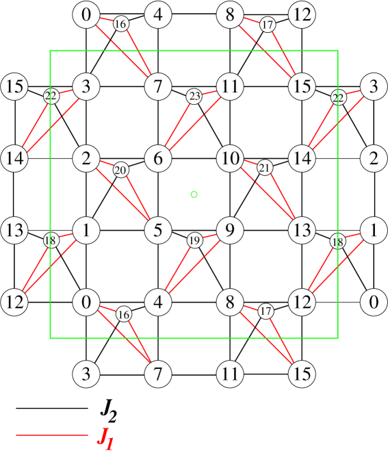
Figure 1: The modified Shastry-Sutherland model on the decorated square lattice for $N=24$ sites (periodic conditions imposed) used for exact diagonalization.

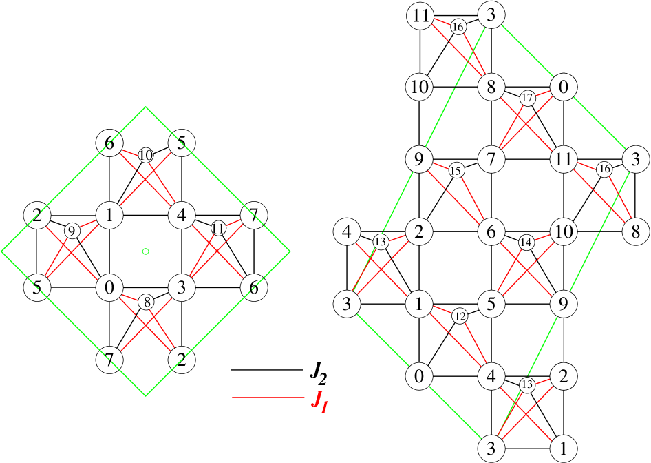
Figure 2: Two finite decorated square lattices of $N=12$ and $N=18$ sites used for exact diagonalization.

3 The model

We consider the inter-spin Heisenberg Hamiltonian on a decorated square-lattice (see figure 1). It results from the well-known Shastry-Sutherland model by replacing its diagonals by equilateral triangles with uniform intra-trimer interaction strength $J_{1}>0$. The set of triangles is divided in a bi-partite fashion into two disjoint subsets of triangles of type I and type II, corresponding to diagonals with positive slope resp. negative ones, see figure 1. Each triangle of, say, type I is surrounded by four triangles of type II and connected to each of them with three bonds of strength $J_{2}$.
It follows that the inter-trimer coupling satisfies the balance condition (5) and hence the theory of TSPGS’s applies. In particular, two questions arise which will be addressed in the following sections: What is the size of the TSPGS-region and of what kind are the lowest excitations? The latter question is also connected to the issue of magnetization plateaus which will be shortly discussed below.

4 Results

4.1 Numerical results

In what follows we set $J_{1}=1$ and consider $J_{2}$ as the variable bond strength. To study the region where the TSPGS is the ground state of the model (4) we use the Lanczos exact diagonalization (ED) technique. Since for spin quantum numbers $s>1/2$ considered here the size of the Hamiltonian matrix grows much faster with system size $N$ than for $s=1/2$, we are restricted to finite lattices of $N=12,18$ and $24$ for $s=1$ and $N=12$ for $s=2$. The largest lattice is shown in figure 1, whereas the smaller lattices are shown in figure 2. Although the criterion for the existence of TSPGS’s (see section 3) are fulfilled, we have to mention that for the small lattices of $N=12$ and $N=18$ the exchange pattern of the $J_{1}$ diagonal bonds in the squares do not match to the infinite system. Nevertheless, we have included the data for $N=12$ and $18$ to get an impression on finite-size effects and on the influence of the spin quantum number $s$.

According to schmidt10 the TSPGS is gapped. Hence we use the spin gap, see figure 3, to detect the critical points $J^{c1}_{2}$ and $J^{c2}_{2}$, where the TSPGS gives way for other ground states. We find for $s=1$ the values $J^{c1}_{2}=-0.570,-0.578$, and $-0.587$ and $J^{c1}_{2}=0.434,0.446$, and $0.454$ for $N=12,18$, and $24$, respectively (cf. figure 3(a)). For $s=2$ and $N=12$ we have $J^{c1}_{2}=-0.400$ and $J^{c2}_{2}=0.322$, cf. figure 3(b). These values lie between the upper and lower bounds which will be derived for $J^{c1}_{2}$ and $J^{c2}_{2}$ in the next section for $N\to\infty$. The nature of the lowest excited state depends on $J_{2}$. Around $J_{2}=0$ it is a triplet state with strong antiferromagnetic correlations along the trimer bonds and weak correlations between the trimers. Near $J^{c1}_{2}$ the lowest excitation is a ferrimagnetic state, i.e. the total spin is $S=Ns/3$ and the system splits into two ferromagnetically correlated sublattices containing on the one hand the $2N/3$ square-lattice sites (i.e. sites $0,1,\ldots,15$ in figure 1) and on the other hand the $N/3$ additional sites (i.e. sites $16,17,\ldots,23$ in figure 1). The spin correlations between both sublattices are anti-ferromagnetic. The ferrimagnetic state is the ground state for $-1.5<J_{2}<J^{c1}_{2}$. Near $J^{c2}_{2}$ the lowest excitation is a collective singlet state with strong correlations along all bonds, and, this state becomes the ground state at $J_{2}=J^{c2}_{2}$.

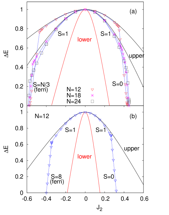
Figure 3: Numerical exact data for $N=12$, $18$, and $24$ (symbols) as well as upper (black solid line) and lower bounds (red solid line) for the excitation gap $\Delta E$. (a) spin quantum number $s=1$; (b) spin quantum number $s=2$. Note that the labels $S=1$, $S=0$, $S=2N/3$ (ferri), and $S=8$ (ferri) characterize the total spin of the excited state.

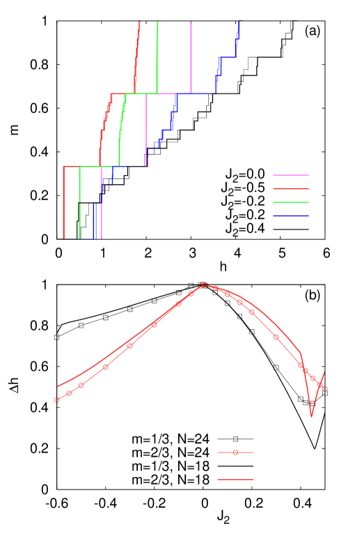
Figure 4: (a) Magnetization curve $m(h)$ for selected values of $J_{2}$ and $s=1$ (thick lines $N=24$, thin lines $N=18$); (b) Plateau widths $\Delta h$ of the $m=1/3$ and the $m=2/3$ plateaus as a function of $J_{2}$ for $N=24$ and $N=18$ and $s=1$.

It is well known that the magnetization curve of the Shastry-Sutherland model (as well as that of the corresponding material SrCu₂(BO₃)₂) possesses a series of plateaus, see, e.g., Kage ; kodama ; misguich ; mila . Motivated by this, we study now briefly the magnetization curve $M(h)$ (where $M$ is the total magnetization and $h$ is the strength of the external magnetic field) for the considered model for $s=1$ using ED for $N=18$ and $N=24$ sites. ED results for the relative magnetization $m=M/M_{sat}$ versus magnetic field $h$ for $N=18$ and $N=24$ sites are shown in figure 4a. Again the finite-size effects seem to be small. Trivially, in the limit $J_{2}=0$ the $m(h)$ curve consists of three equidistant plateaus and jumps according to the magnetization curve of an individual triangle. Switching on a ferromagnetic inter-triangle bond $J_{2}<0$ the general shape of the magnetization curve is preserved. However, the saturation field as well as the end points of the plateaus decrease almost lineraly with $J_{2}$ and become zero at $J_{2}=1.5$, where the ground state becomes the fully polarized ferromagnetic state.

In case of a moderate antiferromagnetic inter-triangle bond $J_{2}>0$ the plateaus at $m=1/3$ and $m=2/3$ still exist, however the discontinuous transition between plateaus becomes smooth. Note that a $m=1/3$ plateau was also found for the standard Shastry-Sutherland model misguich ; mila . The plateau widths $\Delta h$ of the $m=1/3$ and $m=2/3$ plateaus in dependence on $J_{2}$ is shown in figure 4b. Obviously, both widths shrink monotonously with increasing of $|J_{2}|$. If $J_{2}$ approaches the critical value $J^{c1}_{2}$ we find indications for additional plateaus, e.g., at $m=5/6$. Note, however, that our finite-size analysis of the plateaus naturally could miss other plateaus present in infinite systems, see, e.g., the discussion of the ED data of the $m(h)$ curve of the standard Shastry-Sutherland model in wir04 . Hence, the study of the magnetization process of the considered quantum spin model needs further attention based on alternative methods.

One might expect that the presence of these plateaus and jumps may be linked purely to quantum effects because they are often not observed in equivalent classical models at $T=0$ lm ; kawamura ; zhito ; cabra . However, for the present model the plateau at $m=1/3$ survives in the classical limit for $J_{2}<0$ as we will show in appendix B.

4.2 Analytical results

4.2.1 $s=1$

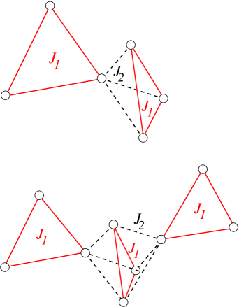
Figure 5: Two possible subsystems of the modified Shastry-Sutherland lattice, see e. g. figure 1. The upper one, $H_{6}$, consists of two coupled triangles; the lower one, $H_{9}$ of three triangles.

In order to obtain analytical results about the TSPGS-region we have adapted theorem $3$ of schmidt10 to the present situation. A slightly more general version of this theorem is stated and proven in appendix A. It yields lower bounds for the gap $\Delta E$ of the form $\Delta E\geq f(4J)$ and the TSPGS-region in terms of properties of simpler spin systems of which the lattice can be composed, see figure 3. These subsystems are chosen here as systems isomorphic to $H_{6}$, see figure 5, consisting of two neighboring triangles. For $s=1$ the gap function $x\equiv\delta_{6}E=f(J),\,J\equiv\frac{J2}{J1}$ of $H_{6}$ is obtained as a special case of equation (7) given below. This yields the corresponding bounds for the TSPGS-region $(J^{c1},J^{c2})$

$$J^{c1}<\frac{3-\sqrt{73}}{16}\approx-0.3465<\frac{1}{4}<J^{c2}\quad\mbox{for }s=1\;.$$ (6)

The function $\delta_{6}E=f(J)$ according to (7) also provides an upper bound for the gap function of the lattice, since it represents the energy of a state orthogonal to the TSPGS, albeit not an eigenstate of $H$. This bound is very close to the numerically determined gap function in the case of $N=12$, see figure 3a, but considerably deviates in the cases of $N=18$ and $N=24$. This indicates that, in general, the lowest excitations of the lattice are different from the excitations of $H_{6}$.

4.2.2 General $s$

It is possible to analytically calculate the energy of the lowest excitations of $H_{6}$ for general integer $s$. The corresponding gap $\delta_{6}E=x=f(J)$ is obtained as the lowest root of the following cubic equation

$$- (x-4)(x-2)(x-1)-(x-1)(2x-5)J$$ (7)

$$+ (1-3r-x+rx)J^{2}+rJ^{3}=0$$

where we have set $r\equiv s(s+1)$. From this result one derives the lower bound

$$\Delta E\geq f(4J)\quad\mbox{for general }s$$ (8)

and a lattice of arbitrary size, see theorem $1$ in appendix A adapted to the system under consideration. The corresponding curves are shrinking in $J$-direction with increasing $s$ and yield inner bounds for the TSPGS-region $(J^{c1},J^{c2})$ of the form

$$J^{c1}<J_{L}^{(1)}<0<J_{L}^{(2)}<J^{c2}\;,$$ (9)

see figure 8 (green curves). Upon scaling w. r. t. the new variable $j\equiv\sqrt{r}J$ the graphs of (7) asymptotically approach the curve given by

$$j^{2}=\frac{(x-4)(x-2)(x-1)}{16(x-3)}\;,$$ (10)

with Taylor expansion

$$x=1-\frac{32}{3}j^{2}+{\mathcal{O}}(j^{3})\;,$$ (11)

see figure 6. Hence $J_{L}^{(i)}$ assumes for $s\to\infty$ asymptotically the form

$$|J_{L}^{(i)}|\sim\frac{1}{\sqrt{6s(s+1)}},\;\;i=1,2\;.$$ (12)

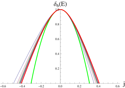
Figure 6: Lower bounds of the scaled gap function $\delta_{6}E(j),\;j=\sqrt{s(s+1)}J$ of the modified Shastry-Sutherland spin lattice for $s=1,\ldots,10$ (thin curves) obtained from Eq. (7). The curves approach the asymptotic (10) for $s\rightarrow\infty$ (thick red curve) which has a simple quadratic approximation (11) (thick green curve).

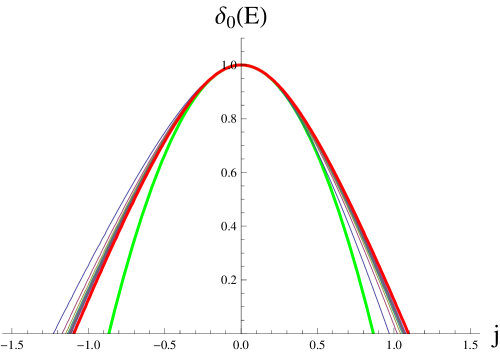
Figure 7: Upper bounds of the scaled gap function $\delta_{0}E(j),\;j=\sqrt{s(s+1)}J$ of the modified Shastry-Sutherland spin lattice for $s=1,\ldots,10$ (thin curves) obtained from Eq. (LABEL:ar6). The curves approach the asymptotic (17) for $s\rightarrow\infty$ (thick red curve) which has a simple quadratic approximation (18) (thick green curve).

In order to obtain close upper bounds $g(J)$ of the gap $\Delta(E)$ in the case $N\geq 18$ we calculate the energy of a certain (degenerate) state that involves three triangles for arbitrary integer $s$, say, one triangle of type $I$ and two neighboring triangles of type $II$, see figure 5. This state is obtained as an exact eigenstate of $H_{0}$, which is the full Hamiltonian $H$, restricted to a $4^{3}=64-$dimensional subspace spanned by product states of the form

$$\phi_{i}\otimes\phi_{j}\otimes\phi_{k},\quad i,j,k=0,\ldots,3\;.$$ (13)

The $\phi_{n}$ live in the $(2s+1)^{3}$-dimensional Hilbert spaces belonging to one of the three triangles. $\phi_{0}=[0,1,2]$ denotes the TSPGS of the corresponding triangle and

$$\phi_{i}\equiv\frac{\!\hbox{}\mathop{\vphantom{s}\smash{s}}\limits_{\sim}\!{}_{0}^{(i)}\phi_{0}}{||\!\hbox{}\mathop{\vphantom{s}\smash{s}}\limits_{\sim}\!{}_{0}^{(i)}\phi_{0}||},\;i=1,2,3\;,$$ (14)

where $\!\hbox{}\mathop{\vphantom{s}\smash{s}}\limits_{\sim}\!{}_{0}^{(i)}$ is the $i$-th component of the spin operator $\!\hbox{}\mathop{\vphantom{\bf s}\smash{\bf s}}\limits_{\sim}\!{}_{0}$ pertaining to the spin site number $0$, an arbitrarily chosen spin site of the corresponding triangle. The gap function of $H_{0}$ will be denoted by $x\equiv\delta_{0}E=g(J)$ and constitutes an upper bound for $\Delta(E)$. It has the following implicit form, using $r\equiv s(s+1)$:

$$0 = -12(x-3)^{2}(x-2)(x-1)-6J(x-3)(x-1)(4x-9)$$

$$+J^{2}(x-3)(9-9x+4r(7x-15))+16J^{3}r(2x-5)\;.$$

Again, the function $g$ belongs to the lowest branch of (LABEL:ar6). The corresponding curves are shrinking in $J$-direction with increasing $s$ and yield outer bounds for the TSPGS-region $(J^{c1},J^{c2})$ of the form

$$J_{U}^{(1)}<J^{c1}<0<J^{c2}<J_{U}^{(2)}\;,$$ (16)

see figure 8 (red curves). Upon scaling w. r. t. the new variable $j\equiv\sqrt{r}J$ the graphs of (LABEL:ar6) asymptotically approach the curve given by

$$j^{2}=\frac{3(x-3)(x-2)(x-1)}{7x-15}\;,$$ (17)

with Taylor expansion

$$x=1-\frac{4}{3}j^{2}+{\mathcal{O}}(j^{3})\;,$$ (18)

see figure 7. Hence $J_{U}^{(i)}$ assumes for $s\to\infty$ asymptotically the form

$$|J_{U}^{(i)}|\sim\sqrt{\frac{6}{5s(s+1)}},\;\;i=1,2\;.$$ (19)

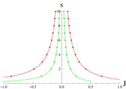
Figure 8: Exact bounds for the TSPGS-region $(J^{c1},J^{c2})$

for $s=1,\ldots,10$ of the form $J_{U}^{(1)}<J^{c1}<J_{L}^{(1)}<0<J_{L}^{(2)}<J^{c2}<J_{U}^{(2)}$. These are derived from (7) (green curves, inner bounds) and (LABEL:ar6) (red curves, outer bounds). In the classical limit $s\rightarrow\infty$ the TSPGS-region shrinks to zero according to (12) and (19).

Although these curves constitute only upper bounds of the true gap functions, the comparison with the numerical results for $N=18$ and $N=24$ reveals a close approximation to both curves, see figure 3. This supports our conjecture that (LABEL:ar6) indeed may serve as an analytical approximation of the gap functions for large $N$ and arbitrary integer $s$. This would mean that the excitations from the TSPGS can be viewed as local excitations essentially concentrated on three neighboring triangles. Numerically determined spin correlation functions seem to be in accordance with this conjecture. Of course, the corresponding excited state will be largely degenerate due to the translational symmetry of the lattice. We expect an almost flat $\bf{k}$-dependance of the energy band $E(\bf{k})$. This expectation is also supported by our numerical results. We have found that the lowest excitations close to $J=0$ have the total spin quantum number $S=1$ in accordance with our model.

In the case $N=12$ where we have performed numerical calculations for $s=1$ and $s=2$ it is not possible to put a subsystem of type $H_{9}$ into the lattice and the above results do not apply. However, an analogous method can be applied to two coupled triangles of type $H_{6}$ and yields an upper bound of the gap function of the form

$$\Delta E\leq\frac{1}{12}(18-3J-\sqrt{9(J-2)^{2}+96J^{2}s(s+1)}).$$ (20)

The numerically determined gap together with the bounds (8) and (20) is represented in figure 3 b.

Appendix A Proof of the gap theorem

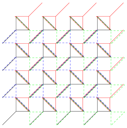
Figure 9: The Hamiltonian of the (modified) Shastry-Sutherland spin lattice can be written as the sum of four classes of simpler Hamiltonians of the kind $H_{6}$, see figure 5, which are indicated by the colors black, red, green, blue. The subsystems of each color are isomorphic via translations $T$ of the lattice. They can be transformed into each other by $90^{\circ}$ rotations $R$ about the mid-points of the empty squares. Note that there are two types of diagonals (trimers), one with positive slope (type I) and the other with negative one (type II). Each diagonal belongs to four subsystems of different color, hence the coupling constant $J_{1}$ of the subsystems, see figure 5, has to be divided by the factor $4$ in order to obtain a total Hamiltonian with the coupling constant $J_{1}$.

In order to prove the existence of an energy gap between the TSPGS and the first excited state we will adapt the analogous proof given in schmidt10 to the modified Shastry-Sutherland model considered in this article. The gap theorem will be formulated in a slightly more general framework.

For any positive integer $\ell$ let ${\mathbb{Z}}_{\bf\ell}$ denote the set of integers modulo $\ell$, such that $n+\ell\equiv n$, and

$${\mathbb{Z}}_{\bf L}={\mathbb{Z}}_{L_{1}}\times\ldots\times{\mathbb{Z}}_{L_{d}}$$ (21)

a standard $d$-dimensional lattice with total size

$${\mathcal{N}}=\prod_{\ell=1}^{d}\;L_{\ell}\;.$$ (22)

We consider an index set ${\mathcal{L}}$ on which the additive group ${\mathbb{Z}}_{\bf L}$ operates effectively, i. e. without fixed points except for the neutral element. Let $c$ be the number of corresponding equivalence classes (orbits), $c=\left|{\mathcal{L}}/{\mathbb{Z}}_{\bf L}\right|$. Each orbit is isomorphic to ${\mathbb{Z}}_{\bf L}$; if we select an index from each orbit we obtain a bijection $\varphi:\{1,\ldots,c\}\times{\mathbb{Z}}_{\bf L}\longrightarrow{\mathcal{L}}$ which we call a “(global) trivialization” in analogy with the corresponding term in the theory of fibre bundles.
We will fix $\tau$ different trivializations

$$\varphi_{\nu}:\{1,\ldots,c\}\times{\mathbb{Z}}_{\bf L}\longrightarrow{\mathcal{L}},\;\nu=1,\ldots,\tau\;.$$ (23)

W. r. t. these trivializations the total Hilbert space can be written as a tensor product space in the following form:

$${\mathcal{H}} = \bigotimes_{i\in{\mathcal{L}}}{\mathcal{H}}_{i}=\bigotimes_{(\ell,{\bf k})\in\{1,\ldots,c\}\times{\mathbb{Z}}_{\bf L}}{\mathcal{H}}_{\varphi_{\nu}(\ell,{\bf k})}$$ (24)

$$= \bigotimes_{{\bf k}\in{\mathbb{Z}}_{\bf L}}\bigotimes_{\ell=1,\ldots,c}{\mathcal{H}}_{\varphi_{\nu}(\ell,{\bf k})}$$ (25)

$$\equiv \bigotimes_{{\bf k}\in{\mathbb{Z}}_{\bf L}}{\mathcal{H}}_{\nu,{\bf k}}\,,\quad\nu=1,\ldots,\tau\;.$$ (26)

We will also write

$${\mathcal{H}}_{\nu,{\bf k}}=\bigotimes_{i\in{\mathcal{S}}_{\nu,{\bf k}}}{\mathcal{H}}_{i}\mbox{ where }{\mathcal{S}}_{\nu,{\bf k}}\equiv\{\varphi_{\nu}(\ell,{\bf k})|1\leq\ell\leq c\}\;.$$ (27)

We will explain these definitions in the case of the modified Shastry-Sutherland model in the finite realization of figure 1. It is a $d=2$-dimensional lattice with $L_{1}=L_{2}=2$, hence ${\mathcal{N}}=L_{1}L_{2}=4$. The $8$ different triangles of figure 1 correspond to the indices $i\in{\mathcal{L}}$, hence ${\mathcal{L}}$ can be viewed as the set of triangles and be identified with the set of numbers of their upper corners $\{16,17,\ldots,23\}$. Note that ${\mathcal{L}}$ is not isomorphic to the underlying spin lattice which has $24$ sites. The Hilbert spaces ${\mathcal{H}}_{i},\;i\in{\mathcal{L}}$ happen to be isomorphic and of the same dimension $(2s+1)^{3}$. In general, it is not necessary that all ${\mathcal{H}}_{i}$ are isomorphic; e. g. we could have spin systems composed of trimers and dimers. ${\mathbb{Z}}_{\bf L}$ operates on ${\mathcal{L}}$ in a natural way by means of translations. Type I triangles $(18,19,22,23)$ cannot be transformed into type II triangles $(16,17,20,21)$ by means of translations. Hence we have, in this case, $c=\left|{\mathcal{L}}/{\mathbb{Z}}_{\bf L}\right|=2$. In figure 9 two adjacent triangles of different types are coupled together in order to form sub-Hamiltonians of the kind $H_{6}$ summing over all possible translations of it. These sub-Hamiltonians are in a $1:1$ manner characterized by trivializations of the kind considered above: We denote the two adjacent triangles we started with by $(1,{\bf 0})$ and $(2,{\bf 0})$, and all other pairs which are translations of these will be denoted by $(1,{\bf k})$ and $(2,{\bf k})$ where ${\bf k}$ runs through ${\mathbb{Z}}_{\bf L}$. Since the set ${\mathcal{L}}$ is exhausted by this construction we have obtained a trivialization in the sense of (23), i. e. a bijection $\varphi_{\nu}:\{1,2\}\times{\mathbb{Z}}_{\bf L}\longrightarrow{\mathcal{L}},\,\nu=1,\ldots,\tau$. In figure 9 $\tau=4$ different trivializations are shown and indicated by different colors.

Returning to the general case we will identify all factor spaces belonging to subsystems of the same type by means of a certain product basis $\{|\gamma\rangle\},\;\gamma:{\mathcal{L}}\longrightarrow{\mathbb{N}}$ in ${\mathcal{H}}$ such that $i\in{\mathcal{L}}\mapsto\gamma(i)\in\{0,\ldots,\mbox{dim}_{i}\}$, where $\mbox{dim}_{i}$ denotes the dimension of ${\mathcal{H}}_{i}$. Correspondingly, the unitary translation operators $T_{\bf m},\;{\bf m}\in{\mathbb{Z}}_{\bf L}$ are defined by suitable permutations of the product basis. W. r. t. a trivialization $\varphi_{\nu}$ this definition assumes the form

$$(T_{\bf m}\,\gamma)(\varphi_{\nu}(\ell,{\bf n}))=\gamma(\varphi_{\nu}(\ell,{\bf m}+{\bf n}))\;.$$ (28)

The $T_{\bf m},{\bf m}\in{\mathbb{Z}}_{\bf L}$ form the abelian translation group ${\mathcal{T}}$ whose characters are of the well-known form

$$\chi(T_{\bf m}) = \exp\left(2\,\pi\,i\,{\bf m}\cdot{\bf k}/{\mathcal{N}}\right),$$ (29)

where $${\bf m}=(m_{1},\ldots,m_{d}),\,{\bf k}=(k_{1},\ldots,k_{d})\in{\mathbb{Z}}_{\bf L}\;.$$ (30)

The total Hamiltonian $H$ is assumed to be a sum of sub-Hamiltonians of the form

$$H=\sum_{\nu=1}^{\tau}\sum_{{\bf k}\in{\mathbb{Z}}_{\bf L}}H_{\nu,{\bf k}}\equiv\sum_{\nu=1}^{\tau}\sum_{{\bf k}\in{\mathbb{Z}}_{\bf L}}T_{\bf k}H_{\nu}T_{\bf k}^{\ast}\;,$$ (31)

where $H_{\nu,{\bf k}}$ is defined on the “supporting factor space” ${\mathcal{H}}_{\nu,{\bf k}}$, see (26), and extended as the identity operator on the remaining factor spaces to the total space ${\mathcal{H}}$. Of course, it suffices to postulate this only for $H_{\nu}=H_{\nu,{\bf 0}}$.

As a consequence of (31) we note that total Hamiltonian will commute with all translations:

$$[H,T_{\bf m}]=0\mbox{ for all }T_{\bf m}\in{\mathcal{T}}\;.$$ (32)

Moreover, we assume the following:

Assumption 1

For all $i\in{\mathcal{L}}$ let $\Phi_{i}\in{\mathcal{H}}_{i}$ be normalized states such that

$$\Phi=\bigotimes_{i\in{\mathcal{L}}}\Phi_{i}$$ (33)

is a ground state of $H_{\nu}$ for all $\nu=1,\ldots,\tau$ which is unique on the factor space ${\mathcal{H}}_{\nu,{\bf 0}}$. We set

$$H_{\nu}\Phi=E_{\nu}^{(0)}\,\Phi$$ (34)

and denote by

$$E_{\nu}^{(1)}=E_{\nu}^{(0)}+\delta_{\nu},\;\delta_{\nu}>0$$ (35)

the next-lowest energy eigenvalue of $H_{\nu}$. Moreover, $\Phi$ is assumed to be invariant under translations,

$$T_{\bf m}\Phi=\Phi\mbox{ for all }T_{\bf m}\in{\mathcal{T}}\;.$$ (36)

Then the gap theorem can be formulated as follows.

Theorem A.1

Under the preceding definitions and assumptions $\Phi$ will be the unique ground state of $H$ with eigenvalue $\tilde{E}_{0}={\mathcal{N}}\,\sum_{\nu=1}^{\tau}E_{\nu}^{(0)}$ and the next-lowest eigenvalue of $H$ satisfies $\tilde{E}_{1}\geq\tilde{E}_{0}+\sum_{\nu=1}^{\tau}\,\delta_{\nu}$.

The existence of a gap follows since $\sum_{\nu=1}^{\tau}\,\delta_{\nu}>0$ is independent of the size ${\mathcal{N}}$ of the lattice. In the special but important case where all $H_{\nu},\;\nu=1,\ldots,\tau$ are unitarily equivalent, we write $E^{(1)}=E^{(0)}+\delta$ and conclude $\tilde{E}_{0}={\mathcal{N}}\,\tau\,E^{(0)}$ and $\tilde{E}_{1}\geq\tilde{E}_{0}+\tau\,\delta$.

Proof of theorem A.1: The first claim (except uniqueness) follows immediately from assumption 1 and the fact that, due to 36, $\Phi$ is also a ground state of all $H_{\nu,{\bf k}}$ with the same eigenvalue $E_{\nu}^{(0)},\;{\bf k}\in{\mathbb{Z}}_{\bf L}$ and ${\mathcal{N}}\,\sum_{\nu=1}^{c}E_{\nu}^{(0)}$ being an obvious lower bound of $H$.
Let $\Psi\in\mathcal{H}$ be the eigenvector of $H$ belonging to the next-lowest eigenvalues $\tilde{E}_{1}\geq\tilde{E}_{0}$. We first note that $\Psi\perp\Phi$ follows in the case $\tilde{E}_{1}>\tilde{E}_{0}$ and can be arranged in the case $\tilde{E}_{1}=\tilde{E}_{0}$ (which we cannot exclude from the outset) by choice of $\Psi$. Moreover, due to (32) we may choose $\Psi$ to be a common eigenvector of all translations,

$$T_{\bf m}\,\Psi=\chi(T_{\bf m})\,\Psi\mbox{ for all }T_{\bf m}\in{\mathcal{T}}\;,$$ (37)

where $\chi(T_{m})$ is of the form (29).

Our aim is to show $\tilde{E}_{1}\geq\tilde{E}_{0}+\sum_{\nu=1}^{c}\,\delta_{\nu}$. Let $|{\alpha}\rangle,\alpha=0,1,2,\ldots$ denote the eigenbasis of $H_{\nu,{\bf k}}$ in ${\mathcal{H}}_{\nu,{\bf k}}$. Further we arrange the eigenbasis such that $|{0}\rangle=\bigotimes_{i\in{\mathcal{S}}_{\nu,{\bf k}}}\,\Phi_{i}$ holds, see (27). The corresponding eigenvalues of $H_{\nu,{\bf k}}$ are denoted by $E_{\nu}^{(\alpha)}$, in accordance to the notation $E_{\nu}^{(0)}$ and $E_{\nu}^{(1)}$ introduced above. $|{\alpha,K}\rangle$ denotes a corresponding product basis in $\mathcal{H}$, where $K$ stands for some multi-index of quantum numbers. Moreover, we consider the reduced density operator $W_{\Psi}^{\nu,{\bf k}}$ in ${\mathcal{H}}_{\nu,{\bf k}}$ defined by the partial trace

$$\langle\alpha|W_{\Psi}^{\nu,{\bf k}}|\beta\rangle=\sum_{K}\langle\alpha,K|\Psi\rangle\langle\Psi|\beta,K\rangle\;.$$ (38)

Then we conclude

$$\tilde{E}_{1} = \langle\Psi|H|\Psi\rangle=\sum_{\nu,{\bf k}}\langle\Psi|H_{\nu,{\bf k}}|\Psi\rangle$$ (39)

$$= \sum_{\nu,{\bf k}}\mbox{Tr}\left(H_{\nu,{\bf k}}\,W_{\Psi}^{\nu,{\bf k}}\right)$$ (40)

$$= \sum_{\nu,{\bf k},\alpha}\mbox{Tr}\left(E_{\nu}^{(\alpha)}|\alpha\rangle\langle\alpha|W_{\Psi}^{\nu,{\bf k}}\right)$$ (41)

$$= \sum_{\nu,{\bf k},\alpha}E_{\nu}^{(\alpha)}\langle\alpha|W_{\Psi}^{\nu,{\bf k}}|\alpha\rangle$$ (42)

$$= \sum_{\nu,{\bf k}}\left(E_{\nu}^{(0)}\langle 0|W_{\Psi}^{\nu,{\bf k}}|0\rangle+\sum_{\alpha>0}E_{\nu}^{(\alpha)}\langle\alpha|W_{\Psi}^{\nu,{\bf k}}|\alpha\rangle\right)$$

$$\geq \sum_{\nu,{\bf k}}\left(E_{\nu}^{(0)}\langle 0|W_{\Psi}^{\nu,{\bf k}}|0\rangle+(E_{\nu}^{(0)}+\delta_{\nu})\sum_{\alpha>0}\langle\alpha|W_{\Psi}^{\nu,{\bf k}}|\alpha\rangle\right)\;.$$

Lemma 1

$$\langle 0|W_{\Psi}^{\nu,{\bf k}}|0\rangle\leq 1-\frac{1}{\mathcal{N}}\;.$$

Proof of lemma 1: It suffices to consider the case ${\bf k}={\bf 0}$. We again consider the product basis $\{|\gamma\rangle\}$ introduced above and write the $c$ quantum numbers $\gamma(\varphi_{\nu}(\ell,{\bf 0})),\;\ell=1,\ldots,c,$ at the first $c$ places of the string $|\gamma\rangle=$
$|n_{1},n_{2},\ldots,n_{c},\ldots\rangle$. It follows that the ground state in ${\mathcal{H}}_{\nu,{\bf 0}}$ is denoted by a ket $|0,0,\ldots,0\rangle$ consisting of $c$ zeroes.

We conclude

$$\langle 0,\ldots,0|W_{\Psi}^{\nu,{\bf 0}}|0,\ldots,0\rangle=\sum_{K}|\langle\Psi|0,\ldots,0,K\rangle|^{2}\equiv s_{0}$$ (45)

and

$$1 = \mbox{Tr}W_{\Psi}^{\nu,{\bf 0}}$$ (46)

$$= \sum_{n_{c+1},n_{c+2},\ldots}|\langle\Psi|0,\ldots,0,n_{c+1},n_{c+2},\ldots\rangle|^{2}$$ (48)

$$+\sum_{n_{1},n_{2},\ldots}|\langle\Psi|n_{1},n_{2},\ldots\rangle|^{2}$$

$$\equiv s_{0}+s_{1}\;.$$ (49)

The first sum $s_{0}$ in (46) runs through all sequences
$0,\ldots,0,n_{c+1},n_{c+2},\ldots$ excluding the value $n_{c+1}=n_{c+2}=\ldots=0$, since $\langle\Psi|\Phi\rangle=0$. Equivalently, we will say that it runs through all states $\psi=|0,\ldots,0,n_{c+1},n_{c+2},\ldots\rangle\in\mathcal{B}_{0}$. The second sum $s_{1}$ in (48) runs through all sequences $n_{1},n_{2},\ldots$ except those with $n_{1}=n_{2}=\ldots=n_{c}=0$, or, equivalently, through all states $\psi=|n_{1},n_{2},\ldots\rangle\in\mathcal{B}_{1}$. Thus the total sum in (46,48) runs through an orthonormal basis $\mathcal{B}=\mathcal{B}_{0}\cup\mathcal{B}_{1}$ of $\mathcal{H}^{\prime}\equiv\{\psi\in\mathcal{H}|\langle\psi|\Phi\rangle=0\}$.
We consider on $\mathcal{B}$ the equivalence relation $\psi_{1}\sim\psi_{2}\Leftrightarrow\psi_{1}=T_{\bf m}\,\psi_{2}$ for some $T_{\bf m}\in{\mathcal{T}},$ and denote by $\Lambda=\mathcal{B}/_{\sim}$ the corresponding set of equivalence classes or “orbits”. Due to (37) all states $\psi$ in the same orbit $\lambda$ yield the same value

$$t_{\lambda}\equiv|\langle\Psi|\psi\rangle|^{2}=|\langle\Psi|T_{\bf m}\,\psi\rangle|^{2},\;T_{\bf m}\in{\mathcal{T}}\;.$$ (50)

For each orbit $\lambda\in\Lambda$ let $N_{\lambda}\equiv|\lambda|$ denote its length. For most orbits we have $N_{\lambda}={\mathcal{N}}$, but in general $N_{\lambda}$ will be a divisor of ${\mathcal{N}}$. For example, if $d=1$, $L_{1}={\mathcal{N}}=6$ and $|1,2,3,1,2,3\rangle\in\lambda$ then $N_{\lambda}=3$. We define $N_{\lambda}^{(k)}\equiv|\lambda\cap\mathcal{B}_{k}|,\;k=0,1,$ and obtain the following equations:

$$N_{\lambda} = N_{\lambda}^{(0)}+N_{\lambda}^{(1)}\;,$$ (51)

$$s_{0} = \sum_{\lambda\in\Lambda}t_{\lambda}\,N_{\lambda}^{(0)}\;,$$ (52)

$$s_{1} = \sum_{\lambda\in\Lambda}t_{\lambda}\,N_{\lambda}^{(1)}\;.$$ (53)

Let $\psi=|n_{1},n_{2},n_{3},n_{4},\ldots\rangle\in\lambda$. Note that at least one $n_{j},\;1\leq j\leq c{\mathcal{N}}$ must be non-zero since $\psi\neq\Phi=|0,0,\ldots,0\rangle$. Hence at least one translation of $\psi$ belongs to $\mathcal{B}_{1}$, namely that where $j$ is shifted to one of the first $c$ places. To show this in detail we write $n_{j}=\gamma(\varphi_{\nu}(\ell,{\bf k})),\;1\leq\ell\leq c,\,{\bf k}\in{\mathbb{Z}}_{\bf L}$. It follows that $T_{-{\bf k}}\psi=|m_{1},m_{2},m_{3},m_{4},\ldots\rangle\in\lambda$ and $m_{\ell}=n_{j}\neq 0$. Thus $N_{\lambda}^{(1)}\geq 1$ and hence $N_{\lambda}^{(0)}\leq N_{\lambda}-1\leq{\mathcal{N}}-1$ which for $\sum_{\lambda\in\Lambda}t_{\lambda}>0$ implies

$$\frac{s_{1}}{s_{0}}\geq\frac{1}{{\mathcal{N}}-1}\;.$$ (54)

$\sum_{\lambda\in\Lambda}t_{\lambda}=0$ is impossible since it would imply that $t_{\lambda}=0$ for all $\lambda\in\Lambda$ and hence $1=s_{0}+s_{1}=0$.
From (54) we infer

$$\frac{1}{s_{0}}=\frac{s_{0}+s_{1}}{s_{0}}=1+\frac{s_{1}}{s_{0}}\geq 1+\frac{1}{{\mathcal{N}}-1}=\frac{{\mathcal{N}}}{{\mathcal{N}}-1}$$ (55)

and

$$s_{0} \leq \frac{{\mathcal{N}}-1}{{\mathcal{N}}}=1-\frac{1}{{\mathcal{N}}}\;,$$ (56)

$$s_{1} \geq \frac{1}{{\mathcal{N}}}\;,$$ (57)

which concludes the proof of the lemma. ∎

To complete the proof of theorem A.1 we use again the eigenbasis of $H_{\nu,{\bf k}}$ and write

$$1=\mbox{Tr }W_{\Psi}^{\nu,{\bf k}}=\langle 0|W_{\Psi}^{\nu,{\bf k}}|0\rangle+\sum_{\alpha=1,2,\ldots}\langle\alpha|W_{\Psi}^{\nu,{\bf k}}|\alpha\rangle=s_{0}+s_{1}\;.$$ (58)

Then we rewrite (LABEL:app15f) as

$$\tilde{E}_{1} \geq \sum_{\nu,{\bf k}}\left(E_{\nu}^{(0)}\,s_{0}+(E_{\nu}^{(0)}+\delta_{\nu})\,s_{1}\right)$$ (59)

$$= \sum_{\nu,{\bf k}}(E_{\nu}^{(0)}+\delta_{\nu}\,s_{1})$$ (60)

$$= \tilde{E}_{0}+{\mathcal{N}}\,\sum_{\nu}\delta_{\nu}\,s_{1}\geq\tilde{E}_{0}+{\mathcal{N}}\,\frac{1}{{\mathcal{N}}}\sum_{\nu}\delta_{\nu}$$ (61)

$$= \tilde{E}_{0}+\sum_{\nu=1}^{\tau}\delta_{\nu}\;,$$ (62)

where we have used (57) which is equivalent to lemma 1. ∎

In order to apply the gap theorem to the modified Shastry-Sutherland lattice we write for the energies of the subsystems $H_{\nu,{\bf k}}$

$$E^{(1)}=E^{(0)}+\delta({\scriptstyle\frac{1}{4}},J_{2})\;.$$ (63)

This has the consequence that the total Hamiltonian will correspond to the coupling constants $J_{1}=1$ and $J_{2}$ since each triangle is contained in four different subsystems, see figure 9. Since $\delta$ is a homogeneous function of $J_{1},\,J_{2}$, i. e. $\delta(\alpha J_{1},\alpha J_{2})=\alpha\,\delta(J_{1},J_{2})$, we may write $\delta(\frac{1}{4},J_{2})=\frac{1}{4}\,\delta(1,4J_{2})$. Hence the gap theorem implies (note that $\tau=4$)

$$\tilde{E}_{0}\geq\tilde{E}_{1}+4\,\frac{1}{4}\,\delta(1,4J_{2})=\tilde{E}_{1}+\delta(1,4J_{2})\;.$$ (64)

Thus the lower bound of the gap is simply obtained by shrinking the graph of the gap function $\delta(1,J_{2})$ of $H_{6}$ into $J_{2}$-direction by a factor $4$.

Appendix B Classical ground states

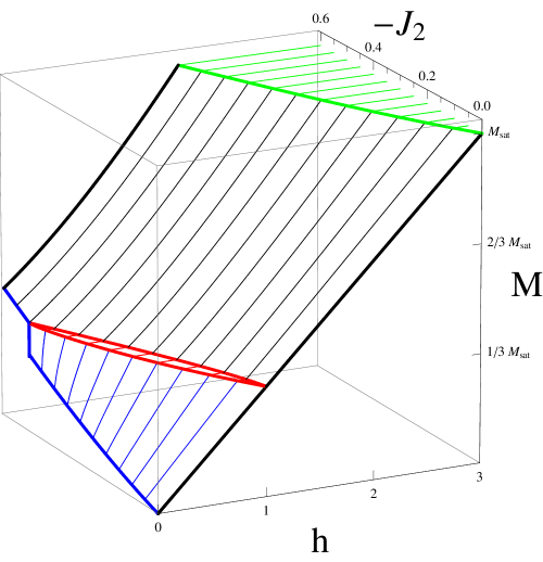
Figure 10: Magnetization curves for the classical modified Shastry-Sutherland lattice for different values of $J=-J_{2}$ between $0$ and $0.6$. The magnetization plateau at $M=\frac{1}{3}M_{\mbox{\scriptsize sat}}$ (indicated by red color) separates states of phase II (blue curves) from those of phase III (black curves). Full magnetization $M=M_{\mbox{\scriptsize sat}}$ is reached in the region indicated by green color. The phase boundaries can be analytically calculated, see (71) - (75).

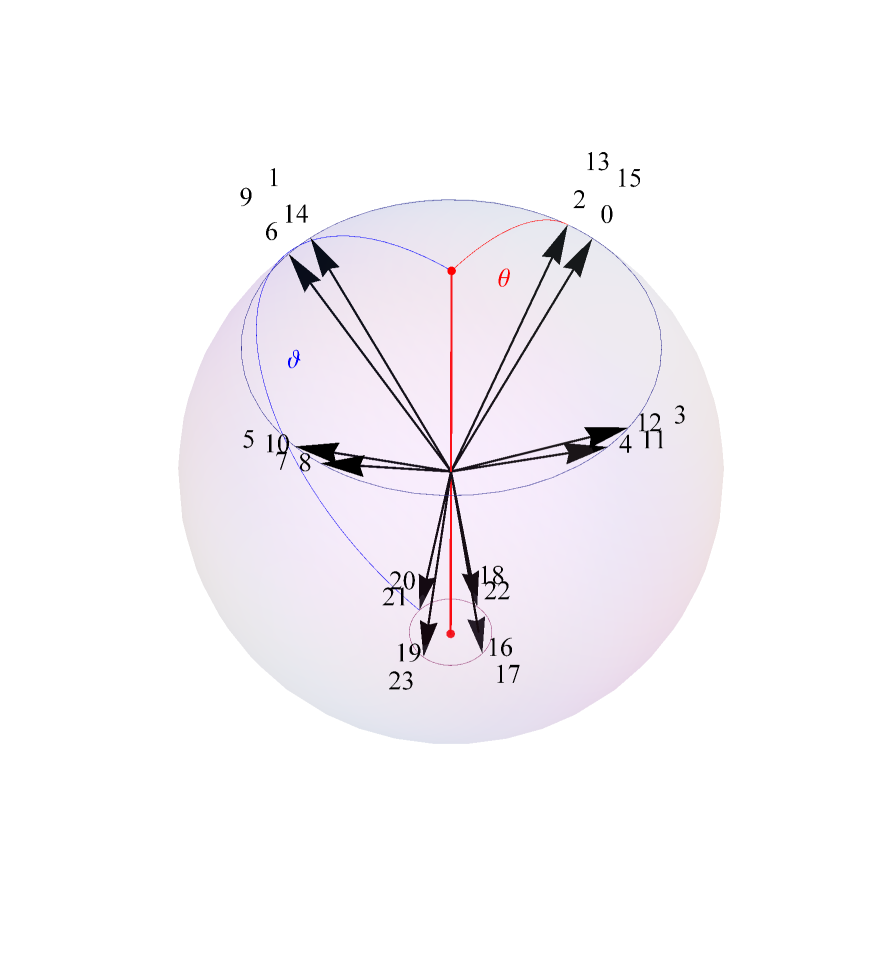
Figure 11: A typical classical ground state of phase II according to (66)-(69). The numbers $\mu$ which are attached to the spin vectors ${\bf s}_{\mu}$ refer to the spin sites of figure 1. All spin vectors of the in-plane spins lie on a cone with opening angle $\theta$, whereas the out-of-plane spins have a polar angle $\vartheta$.

It follows from the general theory schmidt10 as well as from our special results (10) and (17) that the classical modified Shastry-Sutherland model possesses no TSPGS’s except for $J_{2}=0$. Nevertheless it is possible to analytically obtain the classical ground states for $J_{2}\neq 0$ and arbitrary magnetic field $h$ and from these the magnetization curves. Typically in the classical limit $s\rightarrow\infty$ the magnetization curves at $T=0$ are smooth and do not exhibit plateaus or jumps lm ; kawamura ; zhito ; cabra . An exception to this rule is, e. g., reported in schroeder05 . Hence it is remarkable that the classical modified Shastry-Sutherland model possesses a plateau at a magnetization of $M=\frac{1}{3}M_{\mbox{\scriptsize sat}}$ and a jump at $h=0,\;J_{2}=-1/2$, as will be shown in the sequel.

For sake of simplicity we assume a quadratic square lattice of $L\times L$ squares, where $L\geq 4$ is some multiple of $4$. It hence contains $\ell=\frac{L^{2}}{2}$ triangles $\Delta_{\mu},\;\mu=1,\ldots,\ell$. Let ${\bf s}_{\mu,0},\,{\bf s}_{\mu,1},\,{\bf s}_{\mu,2}$ denote the three (unit) spin vectors corresponding to $\Delta_{\mu}$ such that ${\bf s}_{\mu,0}$ corresponds to the “out-of-plane” spin site, see figure 1, and

$${\bf S}_{\mu}={\bf s}_{\mu,0}+{\bf s}_{\mu,1}+{\bf s}_{\mu,2},\quad\mu=1,\ldots,\ell$$ (65)

denote its total spin. $\Delta_{\mu}$ is uniformly coupled to two adjacent sites which belong to neighboring triangles with strength $J_{2}$. As usual, we write the Zeeman term in the Hamiltonian as $-h\,M\equiv-h\,\left(\sum_{\mu=1}^{\ell}{\bf S}_{\mu}\right)_{3}$ where $h$ is the strength of the (dimensionsless) magnetic field. We will confine ourselves to the ferromagnetic case $J_{2}<0$, which shows the most interesting features. In the AF case $J_{2}>0$ the magnetization curves are almost linear until they reach the saturation domain.
As one can see in figure 10 there are, besides the fully aligned state with $M=M_{\mbox{\scriptsize sat}}=3\ell$, exactly three different phases. Phase I which forms the magnetization plateau at $M=\frac{1}{3}M_{\mbox{\scriptsize sat}}=\ell$ is given by the $uud$-state, i. e. in each triangle $\Delta_{\mu}$ the two in-plane spins point into the direction of the magnetic field (“up”) and the off-plane spin in the opposite direction (“down”).
The two other phases II and III have spin vectors of the form

$${\bf s}_{\mu\,i}=\left(\begin{array}[]{c}\sin\theta\,\cos\varphi_{\mu\,i}\\ \sin\theta\,\sin\varphi_{\mu\,i}\\ \cos\theta\end{array}\right),\quad\mu=1,\ldots,\ell,\;i=1,2$$ (66)

and

$${\bf s}_{\mu\,0}=\left(\begin{array}[]{c}\sin\vartheta\,\cos\varphi_{\mu\,0}\\ \sin\vartheta\,\sin\varphi_{\mu\,0}\\ \cos\vartheta\end{array}\right),\quad\mu=1,\ldots,\ell\;.$$ (67)

Ground states of phase II live in the domain $0<M<\frac{1}{3}M_{\mbox{\scriptsize sat}}$ and are visualized in figure 11. Their azimuthal angles $\varphi_{\mu\,i},\,i=1,2$ assume $8$ different values

$$\varphi_{\mu\,i}=n\frac{\pi}{2}\pm\phi,\;n=0,\ldots,3$$ (68)

which depend on a parameter $\phi$, whereas

$$\varphi_{\mu\,0}=n\frac{\pi}{2},\;n=0,\ldots,3\;.$$ (69)

Upon a translation from, say, the triangle $(0,7,16)$ to $(4,9,19)$, see figure 1, the azimuthal angles (68) and (69) are shifted by an amount of $-\frac{\pi}{2}$. Hence the states of phase II are characterized by a wave number of $k=\frac{\pi}{2}$ (the minus sign does not matter). If the magnetic field $h$ approaches the left hand boundary of the $M=\frac{1}{3}M_{\mbox{\scriptsize sat}}$ plateau, the states of phase II become the $uud$-state. Phase III is confined to a magnetization $M$ satisfying $\frac{1}{3}M_{\mbox{\scriptsize sat}}<M<M_{\mbox{\scriptsize sat}}$. The corresponding states have a wave number $k=\pi$, since their azimuthal angles satisfy $\varphi_{\mu\,i}\in\{0,\pi\}$ for $\mu=1,\ldots,\ell$ and $i=1,2,3$. More precisely, the spins in figure 1 with the numbers $0,2,5,7,8,10,13,15;18,19,22,23$ have an azimuthal angle of $\varphi=0$, and the remaining spins of $\varphi=\pi$.
It is obvious how to generalize the states of phase I, II, III to infinite modified Shastry-Sutherland lattices by periodic continuation. The (semi-)analytical treatment of these states can be based on the ground state equation, see schmidt03 ,

$${\bf j}_{\mu}\equiv\sum_{\nu}J_{\mu\nu}{\bf s}_{\nu}-\left(\begin{array}[]{c}0\\ 0\\ h\end{array}\right)=\kappa_{\mu}\,{\bf s}_{\mu},\quad\mu=1,\ldots,N\;.$$ (70)

Note that here Greek indices $\mu,\nu=1,\ldots,N$ do not number triangles but all spins of a finite spin lattices. The $\kappa_{\mu}$ denote Lagrange parameters due to the constraints ${\bf s}_{\mu}\cdot{\bf s}_{\mu}=1$. They can be eliminated by writing ${\bf j}_{\mu}\times{\bf s}_{\mu}={\bf 0},\;\mu=1,\ldots,N$. These equations, together with the corresponding periodicity properties of phase II or III states, are sufficient to determine the unknowns $\theta,\,\vartheta$ and, for phase II states, $\phi$, as solutions of certain algebraic equations that contain $J_{2}$ and $h$ as parameters. We have calculated the magnetization curves of figure 10 by means of numerical solutions of these equations and checked the results by a direct numerical calculation of the ground states for different $h$ and $J$. For $h=0$ we found a large degenerate set of ground states with total spin $S$ varying between $0$ and some $S_{\mbox{\scriptsize max}}$. In the limit $h\rightarrow 0$ only the states with $S=S_{\mbox{\scriptsize max}}$ are obtained as ground states with finite magnetization $M=S_{\mbox{\scriptsize max}}$.

Actually, the phase boundaries, displayed in figure 10 by thick lines, can be given in closed form. We will write $J=-J_{2}$ and remind the reader of $J_{1}=1$ and $\ell=\frac{L^{2}}{2}=\frac{1}{3}M_{\mbox{\scriptsize sat}}$. The curve for $h\rightarrow 0$ (thick blue curve in figure 10) consists of three parts, the phase II part

$$M_{II}(J)=\ell\,J\,\sqrt{1+2J},\quad 0\leq J\leq\frac{1}{2}\;,$$ (71)

the phase III part

$$M_{III}(J)=\frac{\ell}{2}\,\sqrt{J(1+2J)(3+2J)},\quad\frac{1}{2}\leq J<\frac{3}{2}\;,$$ (72)

and a jump at $J=\frac{1}{2}$ from $M_{1}=\ell\frac{\sqrt{2}}{2}$ to $M_{2}=\ell$.
The saturation field $h_{\mbox{\scriptsize sat}}(J)$ (thick green curve in figure 10) is given by

$$h_{\mbox{\scriptsize sat}}(J)=\frac{1}{2}\left(3-11J+\sqrt{3(3+10J+19J^{2})}\right),\,0\leq J\leq\frac{3}{2}\;.$$ (73)

The value $h_{\mbox{\scriptsize sat}}(0)=3$ is part of the linear magnetization curve for $J_{2}=0$ (thick black line in figure 10) $M(h)=\ell\,h$ which corresponds to the magnetization of a uniform AF triangle.
The two boundaries (72) and (73) meet at the point $h=0,\,J=\frac{3}{2},\,M=M_{\mbox{\scriptsize sat}}=3\ell$.

Finally, the plateau at $M=\frac{1}{3}M_{\mbox{\scriptsize sat}}$ (bounded by thick red curves in figure 10) is given by the inequalities $h_{II}(J)\leq h\leq h_{III}(J)$ where $h_{II}(J)$ is the lower positive root of

$$h(h-1)^{2}+4(h-1)(2h-1)J+(19h-16)J^{2}+16J^{3}=0$$ (74)

in the interval $0\leq J\leq\frac{1}{2}$ and

$$h_{III}(J)=\frac{1}{2}\left(1-9J+\sqrt{1+14J+17J^{2}}\right),\quad 0\leq J\leq\frac{1}{2}\;.$$ (75)

Obviously, the graphs of $h_{II}$ and $h_{III}$ intersect at the two points $J=0,\,h=1$ and $J=\frac{1}{2},\,h=0$.

References

- (1) Quantum Magnetism, U. Schollwöck, J. Richter, D.J.J. Farnell, and R.F. Bishop, Eds. (Lecture Notes in Physics 645, Springer, Berlin, 2004)
- (2) Introduction to Frustrated Magnetism, C. Lacroix, P. Mendels, and J. Mila, Eds. 2011 Introduction to Frustrated Magnetism (Springer Series in Solid-State Sciences, vol. 164) (Springer, Berlin, 2011)
- (3) R. Moessner, Can. J. Phys. 79, 1283 (2001).
- (4) C. Castelnovo, R. Moessner, S. L. Sondhi, Nature 451, 42 (2008).
- (5) L. Balents, Nature 464, 199 (2010).
- (6) D.C. Mattis, The Theory of Magnetism I, Springer, Berlin, 1991
- (7) R.O. Kuzian and S.-L. Drechsler, Phys. Rev. B 75, 024401 (2007).
- (8) M. Zhitomirsky and H. Tsunetsugu, Europhys. Lett. 92, 37001 (2010).
- (9) S.-L. Drechsler, S. Nishimoto, R. Kuzian, J. Málek, J. Richter, J. v. d. Brink, M. Schmitt, and H. Rosner, Phys. Rev. Lett. 106, 219701 (2011).
- (10) H.A. Bethe, Z. Phys. 71, 205 (1931).
- (11) C.K. Majumdar and D.K. Ghosh, J. Math. Phys. 10, 1399 (1969).
- (12) B.S. Shastry and B. Sutherland, Physica B 108, 1069 (1981).
- (13) M. Albrecht and F. Mila, Europhys. Lett. 34, 145 (1996).
- (14) S. Miyahara, K. Ueda, Phys. Rev. Lett. 82, 3701 (1999).
- (15) A. Läuchli, S. Wessel, and M. Sigrist, Phys. Rev. B 66, 014401 (2002).
- (16) C. Knetter and G. S. Uhrig, Phys. Rev. Lett. 92, 027204 (2004).
- (17) R. Darradi, J. Richter, and D.J.J. Farnell, Phys. Rev. B 72, 104425 (2005).
- (18) A. Pimpinelli, J. Phys.: Condens. Matter 3, 445 (1991).
- (19) N.B. Ivanov and J. Richter, Phys. Lett. A 232, 308 (1997); J. Richter, N.B. Ivanov and J. Schulenburg, J. Phys.: Condens. Matter 10, 3635 (1998).
- (20) K. Ueda and S. Miyahara, J. Phys.: Condens. Matter 11, L175 (1999).
- (21) A. Koga, K. Okunishi, and N. Kawakami, Phys. Rev. B 62, 5558 (2002); A. Koga and N. Kawakami, Phys. Rev. B 65, 214415 (2002).
- (22) J. Schulenburg and J. Richter, Phys. Rev. B 65, 054420 (2002).
- (23) H.-J. Schmidt, J. Phys. A: Math. Gen. 38, 2123 (2005).
- (24) G. Müller and R.E. Shrock, Phys. Rev. 32, 5845 (1985).
- (25) J. Schulenburg, A. Honecker, J. Schnack, J. Richter, and H.-J. Schmidt, Phys. Rev. Lett. 88, 167207 (2002); J. Richter, O. Derzhko, and J. Schulenburg, Phys. Rev. Lett. 93, 107206 (2004), M. E. Zhitomirsky and H. Tsunetsugu, Phys. Rev. B 70, 100403(R) (2004); O. Derzhko and J. Richter, Phys. Rev. B 70, 104415 (2004); Eur. Phys. J. B 52, 23 (2006); M. E. Zhitomirsky and H. Tsunetsugu, Phys. Rev. B 75, 224416 (2007).
- (26) M. Gaudin, J. Phys. France 37, 1087 (1976); La Fonction D’onde de Bethe Masson, Paris, 1983; J. Richter an A. Voigt, J. Phys. A.: Math. Gen. 27, 1139 (1994), M. Bortz, S. Eggert, and J. Stolze, Phys. Rev. B 81, 035315 (2010).
- (27) H. Kageyama , K. Yoshimura, R. Stern , N.V. Mushnikov, K. Onizuka, M. Kato, K. Kosuge, C.P. Slichter, T. Goto and Y. Ueda, Phys. Rev. Lett. 82, 3168 (1999).
- (28) S. Miyahara and K. Ueda, Phys. Rev. Lett. 82, 3701 (1999).
- (29) D. Poilblanc, J. Riera, C.A. Hayward, C. Berthier, and M. Horvatic, Phys. Rev. B 55, R11941 (1997).
- (30) Y.-Z. Zheng, M.-L. Tong, W. Xue, W.-X. Zhang, X.-M. Chen, F. Grandjean, and G. J. Long, Angew. Chem. Int. Ed. 46, 6076 (2007).
- (31) J. Richter, J. Schulenburg, A. Honecker, and D. Schmalfuß, Phys. Rev. B 70, 174454 (2004); G. Misguich and P. Sindzingre, J. Phys.: Condens. Matter 19, 145202 (2007); B.-J. Yang, A. Paramekanti, and Y. B. Kim, Phys. Rev. B 81, 134418 (2010).
- (32) H.-J. Schmidt and J. Richter, J. Phys. A.: Math. Theor. 43, 405205 (2010).
- (33) K. Kodama, M. Takigawa, M. Horvatic, C. Berthier, H. Kageyama, Y. Ueda, S. Miyahara, F. Becca, F. Mila, Science 298, 395 (2002).
- (34) G. Misguich, Th. Jolicoeur, and S. M. Girvin, Phys. Rev. Lett. 87, 097203 (2001).
- (35) J. Dorier, K.P. Schmidt, and F. Mila, Phys. Rev. Lett. 101, 250402 (2008).
- (36) J. Richter, J. Schulenburg and A. Honecker, in Quantum Magnetism, eds U. Schollwöck, J. Richter, D.J.J. Farnell, and R.F. Bishop, Lecture Notes in Physics 645 (Springer-Verlag, Berlin, 2004), p. 85.
- (37) H. Kawamura and S. Miyashita, J. Phys. Soc. Jpn. 54, 4530 (1985).
- (38) M.E. Zhitomirsky, A. Honecker, and O.A. Petrenko, Phys. Rev. Lett. 85, 3269 (2000); M.E. Zhitomirsky, Phys. Rev. Lett. 88, 057204 (2002).
- (39) M. Moliner, D.C. Cabra, A. Honecker, P. Pujol, F. Stauffer, Phys. Rev. B 79, 144401 (2009).
- (40) C. Schröder, H.-J. Schmidt, J. Schnack and M. Luban, Phys. Rev. Lett. 94, 207203 (2005).
- (41) H.-J. Schmidt and M. Luban, J. Phys. A.: Math. Theor. 36, 6351 (2003).