Scalar Decay Constant and Yukawa Coupling
in Walking Technicolor Models

Abstract

Based on Refs. Hashimoto:2011ma and Hashimoto:2011cw, we study the couplings of the scalar bound state to the fermions and the weak bosons in walking gauge theories.

1 Introduction

Recently, a modest excess of events around the Higgs mass, $m_{h}\sim 125$ GeV, over the standard model (SM) background has been reported [3]. This Higgs mass is consistent with the precision measurements [4]. I would like to mention, however, it is not yet conclusive. The mechanism for the electroweak symmetry breaking is still unrevealed.

Based on Refs. Hashimoto:2011ma and Hashimoto:2011cw, we study the couplings of the scalar bound state, so-called the technidilaton (TD), to the SM fermions and the weak bosons in walking technicolor (WTC). These are crucial for the TD searches.

2 Coupling to the SM fermions

Suppose that the extended technicolor (ETC) sector generates the four-fermion interaction and that the SM fermion mass $m_{f}$ is obtained from the technifermion (TF) condensate, $\langle\bar{\psi}\psi\rangle$. See also Fig. 1. By introducing the scalar decay constant $F_{S}$ for the scalar current, $\langle 0|(\bar{\psi}\psi(0))_{R}|\sigma(q)\rangle\equiv F_{S}M_{\sigma}$, where $M_{\sigma}$ is the mass of the scalar bound state $\sigma$ and the subscript $R$ represents the renormalized quantity, we can then obtain the yukawa coupling [1],

$$g_{\sigma ff}=\frac{m_{f}}{\frac{-\langle\bar{\psi}\psi\rangle_{R}}{F_{S}M_{\sigma}}}\,.$$ (1)

Figure 1: Yukawa coupling between the SM fermions $f$ and the scalar bound state $\sigma$ in ETC. The TF loop generates the mass of $f$ and also intermediates between $f$ and $\sigma$.

We perform the calculations of $F_{S}$ and $\langle\bar{\psi}\psi\rangle_{R}$ by using the improved ladder SD equation [5]. We then obtain

$$\frac{g_{\sigma ff}}{g_{hff}^{\rm SM}}=\sqrt{\frac{N_{\rm TC}}{N_{f}}}N_{D}\frac{\kappa_{F}^{2}\sqrt{5-\tilde{\omega}^{2}}}{4\pi\sqrt{2\kappa_{V}}}\frac{M_{\sigma}}{v},$$ (2)

where the SM yukawa coupling is $g_{hff}^{\rm SM}=m_{f}/v$ with $v=246$ GeV. Also, $N_{\rm TC}$, $N_{f}$ and $N_{D}$ denote the number of the color of the TC gauge group, the number of the flavor and the weak doublets for each TC index, respectively. The values of $\kappa_{F}$ and $\kappa_{V}$ are defined by

$$v^{2}=N_{D}F_{\pi}^{2}\equiv\frac{N_{\rm TC}N_{D}}{4\pi^{2}}\,\kappa_{F}^{2}\,m^{2},\quad\mbox{and}\quad\langle\theta_{\mu}^{\mu}\rangle\equiv-\frac{N_{\rm TC}N_{f}}{2\pi^{2}}\kappa_{V}m^{4},$$ (3)

where $m$ is the dynamically generated TF mass. We show the numerical values of $g_{\sigma ff}/g_{hff}^{\rm SM}$ in Table 1. We here used the WTC relation $N_{f}\simeq 4N_{\rm TC}$ and $\Lambda_{\rm ETC}$ represents the ETC scale. The values of $\tilde{\omega}$ are obtained through those of $\lambda_{*}$, $\tilde{\omega}\equiv\sqrt{4\lambda_{*}-1}$.

$$\begin{array}[]{c|c|c|c||c||c}\hline\cr\lambda_{*}&\frac{m}{\Lambda_{\rm ETC}}&\kappa_{V}&\kappa_{F}&\sqrt{\frac{N_{D}}{N_{f}}}\frac{F_{S}}{v}&\frac{g_{\sigma ff}}{g_{hff}^{\rm SM}}\frac{v}{N_{D}M_{\sigma}}\\ \hline\cr 0.305&1.12\times 10^{-3}&0.685&1.38&2.59&0.142\\ 0.287&1.08\times 10^{-4}&0.709&1.42&2.71&0.148\\ 0.258&5.88\times 10^{-10}&0.756&1.48&2.93&0.157\\ \hline\cr\end{array}$$

Table 1.   Numerical values of $g_{\sigma ff}/g_{hff}^{\rm SM}$ .

For the typical one-family TC model with $N_{\rm TC}=2$, $N_{f}=8$ and $N_{D}=4$, we can read $m=$ 390 GeV, 380 GeV, 370 GeV from top to bottom in Table 1. The handy Higgs mass formula [6], $M_{\sigma}\simeq\sqrt{2}m$, then yields $M_{\sigma}\simeq$ 560 GeV, 540 GeV, 520 GeV, respectively. For the typical Higgs mass, $M_{\sigma}=$ 500 GeV, we obtain $g_{\sigma ff}/g_{hff}^{\rm SM}\simeq 1.2$. Furthermore, there are $2N_{\rm TC}\;(=4)$ extra colored fermions (techniquarks). Therefore the production cross section of $\sigma$ in such a model should be considerably enhanced, like in the fourth generation models [7]. It has been severely constrained by the recent LHC data [3]. On the other hand, it is not the case for the model having only one weak doublet and no extra techniquark. We also note that signatures of some classes of the top condensate models [8] are similar to the SM.

3 Coupling to the weak bosons

We may regard the scalar bound state $\sigma$ as a dilaton.

When the dilaton $\sigma$ directly couples to $W$, like in the SM, one can easily derive the $\sigma$–$W$–$W$ coupling as [9]

$$g_{\sigma WW}=\frac{2M_{W}^{2}}{F_{\sigma}},$$ (4)

where $F_{\sigma}$ represents the dilaton decay constant being $\langle 0|\theta_{\lambda}^{\lambda}(0)|\sigma(q)\rangle=F_{\sigma}M_{\sigma}^{2}$. Notice that $F_{S}$ in the previous section is different from $F_{\sigma}$.

Next, we consider the situation that the TD couples to the weak bosons only through the TF loop.

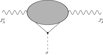
Figure 2: Coupling of the TD to the axial current $J_{A}^{\mu}$ of the TF. The TD couples to $J_{A}^{\mu}$ only through the internal TF lines.

Since the axial current $J_{A}^{\mu}$ of the TF’s yields the decay constant $F_{\pi}$, $\langle 0|J_{A}^{\mu}(0)|\pi(q)\rangle=-iq^{\mu}F_{\pi}$, and the weak boson mass is provided by $F_{\pi}$, the coupling between $\sigma$ and $J_{A}^{\mu}$ should be crucial. See also Fig. 2.

The axial current correlator in the momentum space is

$${\rm F.T.}i\langle 0|J_{A}^{\mu}(x)J_{A}^{\nu}(0)|0\rangle=\left(g^{\mu\nu}-\frac{q^{\mu}q^{\nu}}{q^{2}}\right)\Pi_{A}(q^{2}),\quad\mbox{and}\quad\Pi_{A}(0)=F_{\pi}^{2},$$ (5)

which plays an important role in our approach.

The $\sigma$ coupling to $J_{A}^{\mu}$ at the zero momentum transfer is just like the mass insertion: Note that the identity holds

$$\frac{1}{\hbox to0.0pt{\hbox to5.00002pt{\hfil$\ell$\hfil}\hss}/-m}y_{T}\frac{1}{\hbox to0.0pt{\hbox to5.00002pt{\hfil$\ell$\hfil}\hss}/-m}=y_{T}\frac{\partial}{\partial m}\frac{1}{\hbox to0.0pt{\hbox to5.00002pt{\hfil$\ell$\hfil}\hss}/-m},$$ (6)

where $y_{T}$ represents the yukawa coupling between the TD and the TF. We can then obtain the coupling of $\sigma$ to $J_{A}^{\mu}$ at zero momentum simply by

$$g_{\sigma AA}(0)=y_{T}\frac{\partial\Pi_{A}(0)}{\partial m}\,.$$ (7)

Because $F_{\pi}$ is expected to be proportional to $m$, i.e., $F_{\pi}=\kappa\,m$, with $\kappa\equiv\kappa_{F}\sqrt{N_{\rm TC}}/(2\pi)$ and $\kappa_{F}\simeq 1.4\mbox{--}1.5$ in Eq. (3), Eqs. (5) and (7) then yield $g_{\sigma AA}(0)=y_{T}\cdot 2F_{\pi}^{2}/m$. Attaching $W^{\mu}$ to $J_{A}^{\mu}$, we finally obtain the coupling of the TD to the weak bosons at zero momentum,

$$g_{\sigma WW}(0)=y_{T}\frac{2M_{W}^{2}}{m}\,.$$ (8)

When the yukawa coupling is like the SM, $y_{T}=m/F_{\sigma}$, Eq. (8) formally agrees with Eq. (4). For the model in Ref. Bando:1986bg, where the four-fermion interactions were incorporated, $y_{T}$ was estimated as $y_{T}=(3-\gamma_{m})m/F_{\sigma}$ with $\gamma_{m}\simeq 1$. If so, $g_{\sigma WW}$ is changed by the additional factor $(3-\gamma_{m})$. In any case, we conclude that the (effectively induced) operator $\frac{\sigma}{F_{\sigma}}W_{\mu}W^{\mu}$ yields the coupling between the TD and the weak bosons, similarly to the SM.

4 Summary

We studied the couplings of $\sigma$ to $f$ and $W$. For details, see Refs. Hashimoto:2011ma and Hashimoto:2011cw.

References

• [1] M. Hashimoto, Phys. Rev. D 83, 096003 (2011).
• [2] M. Hashimoto, Phys. Rev. D 84, 111901 (2011).
• [3] ATLAS Collaboration, arXiv:1202.1408 [hep-ex]; CMS Collaboration, arXiv:1202.1488 [hep-ex].
• [4] K. Nakamura et al. [Particle Data Group], J. Phys. G 37, 075021 (2010).
• [5] M. Hashimoto and K. Yamawaki, Phys. Rev. D 83, 015008 (2011).
• [6] M. Hashimoto, Phys. Lett. B 441, 389 (1998).
• [7] P. H. Frampton, P. Q. Hung and M. Sher, Phys. Rept. 330, 263 (2000); H. J. He, N. Polonsky and S. f. Su, Phys. Rev. D 64, 053004 (2001); G. D. Kribs, T. Plehn, M. Spannowsky and T. M. P. Tait, Phys. Rev. D 76, 075016 (2007); M. Hashimoto, Phys. Rev. D 81, 075023 (2010).
• [8] C. T. Hill and E. H. Simmons, Phys. Rept. 381, 235 (2003); Erratum-ibid. 390, 553 (2004); M. Hashimoto, M. Tanabashi and K. Yamawaki, Phys. Rev. D 64, 056003 (2001); ibid D 69, 076004 (2004); V. Gusynin, M. Hashimoto, M. Tanabashi and K. Yamawaki, Phys. Rev. D 65, 116008 (2002).
• [9] W. D. Goldberger, B. Grinstein and W. Skiba, Phys. Rev. Lett. 100, 111802 (2008); J. Fan, W. D. Goldberger, A. Ross and W. Skiba, Phys. Rev. D 79, 035017 (2009).
• [10] M. Bando, K. Matumoto and K. Yamawaki, Phys. Lett. B 178, 308 (1986).