Uncovering the formation of ultra-compact dwarf galaxies by multivariate statistical analysis

Abstract

We present a statistical analysis of the properties of a large sample of dynamically hot old stellar systems, from globular clusters to giant ellipticals, which was performed in order to investigate the origin of ultra-compact dwarf galaxies. The data were mostly drawn from Forbes et al. (2008). We recalculated some of the effective radii, computed mean surface brightnesses and mass-to-light-ratios, estimated ages and metallicities. We completed the sample with globular clusters of M31. We used a multivariate statistical technique (K-Means clustering), together with a new algorithm (Gap Statistics) for finding the optimum number of homogeneous sub-groups in the sample, using a total of six parameters (absolute magnitude, effective radius, virial mass-to-light ratio, stellar mass-to-light ratio and metallicity). We found six groups. FK1 and FK5 are composed of high- and low-mass elliptical galaxies respectively. FK3 and FK6 are composed of high-metallicity and low-metallicity objects, respectively, and both include globular clusters and ultra-compact dwarf galaxies. Two very small groups, FK2 and FK4, are composed of Local Group dwarf spheroidals. Our groups differ in their mean masses and virial mass-to-light ratios. The relations between these two parameters are also different for the various groups. The probability density distributions of metallicity for the four groups of galaxies is similar to that of the globular clusters and UCDs. The brightest low-metallicity globular clusters and ultra-compact dwarf galaxies tend to follow the mass-metallicity relation like elliptical galaxies. The objects of FK3 are more metal-rich per unit effective luminosity density than high-mass ellipticals.

1 Introduction

The variety of astrophysical structures in the Universe, from galaxies and galaxy clusters to stellar remnants, is well described by essential physical principles (Padmanabhan, 2000). However, their origin, in particular that of globular clusters (hereafter GCs), is still a matter of debate. GCs are an intermediate cell of structure between stars and galaxies, and their formation process is a cornerstone for our understanding the Universe (Peebles, 1969; Ashman & Zepf, 1992; Harris et al., 1995; Côté et al., 1998). If we consider star clusters as a single class of astrophysical objects, there are many well-known and poorly understood phenomena, which make their origin enigmatic. For example, the color bimodality of GC systems existing in most galaxies, the absence of a clear mass-metallicity relation for the population of red GCs, the correlation between color and integrated magnitude among the brighter metal-poor GCs (Strader & Smith, 2008), the differences in luminosity functions and surface density profiles between young and old cluster systems (e.g. Brodie & Strader, 2006; Lee et al., 2010, and references therein). Spherical stellar systems, whether globular clusters, elliptical galaxies, or substructures of spiral galaxies, are considered virialized (Antonov, 1973). The origin of GCs is ultimately linked to the evolution of larger pressure-supported structures within the cosmological hierarchy (e.g. Hwang et al., 2008, and references therein).

In the last decade a new type of astronomical object has been discovered by a number of astrophysicists (Hilker et al., 1999; Phillipps et al., 2001; Drinkwater et al., 2000, 2003; Mieske et al., 2006) while making a spectroscopic survey in the Fornax cluster. These objects called ultra-compact dwarf galaxies (UCDs), dwarf globular transition objects or sometimes intermediate massive objects, are different from the classical globular clusters or dwarf elliptical galaxies in terms of their radii, relaxation time and V-band mass-to-light ratios. They are more massive, more luminous, and have higher mass-to-light ratio than globular clusters, but are fainter and more compact than dwarf elliptical galaxies.

Several formation scenario have been proposed for understanding their physical properties. Kroupa (1998) and Fellhauer & Kroupa (2002) suggested that UCDs are the results of merger of many young star clusters formed in galaxy-galaxy encounters whereas Mieske et al. (2002) suggested that they are the luminous extension of massive GCs. The formation of UCDs from the mass threshing of the envelopes of nucleated galaxies has also been suggested (Bassino et al., 1994; Zinnecker et al., 1988; Bekki et al., 2003; Goerdt et al., 2008) while along another line of thought UCDs are considered fundamental building blocks of galaxies (Drinkwater et al., 2004). Special efforts were made to unite old dynamically hot stellar systems, from GCs, UCDs and dwarf spheroidals (dSphs) to giant elliptical galaxies (Zaritsky et al., 2006; Forbes et al., 2008; Dabringhausen et al., 2008) to reveal the nature of UCDs. (Mieske & Kroupa, 2008) have studied the internal dynamics of a large sample of UCDs in Fornax. They argue that UCDs are dynamically unrelaxed and dynamical evolution has probably not influenced their present dynamical M/L ratio.

All these findings originated while studying two-point correlations between different projections of the fundamental plane of galaxies (FP) defined by velocity dispersion, size (or effective radius) and surface brightness (or mass density). For example, relations were found between size and luminosity, mass and metallicity, mass-to-light ratio and dynamical mass, luminosity and velocity dispersion etc. Considering two parameters at a time means disregarding the combining effects of others which in turn are responsible for losing significant information.

For a unique and robust theory of the formation of UCDs, a multivariate approach is more appropriate. The present work is based on a data set covering a broad spectrum of objects, including Galactic and extragalactic GCs, UCDs, young massive star clusters, nuclei of dwarf ellipticals and pressure-supported galaxies, presented in Section 2. We have used the multivariate statistical method of K-Means cluster analysis (presented in Section 3), to classify these diverse objects with respect to a set of physical parameters. Six homogeneous groups have been identified by this objective method, they are described in Section 4, and their properties have been studied by several two-point correlations and regressions (Section 5). Finally conclusions have been drawn in Section 6.

2 The data

The present sample is composed of 370 objects from the paper of Forbes et al. (2008), hereafter F08, to which we added 19 GCs in M31. We did not use all objects of F08 because we were not able to document all the values of the additional parameters (age, metallicity, colors) used in the present study. We took the distance, central velocity dispersion $\sigma_{o}$, effective radius $R_{h}$ and apparent K magnitude $m_{K}$ from Table 1 of F08. We did not use the $R_{h}$ values of the galaxies given in Table 1 of F08 as they did not agree with Fig.3 of F08. Instead we recalculated $R_{h}$ using $R_{20}$ following the method outlined in F08. To that end we needed the axis ratio of the galaxies. We obtained $R_{25}$ from the hyperleda database. $logR_{25}$ is the logarithm of the axis ratio at the isophote 25 mag/$arcsec^{2}$ in the B band. It was available for all galaxies except two (NGC1273 and PER195), which were removed from the sample. The $R_{h}$ values that we obtained agree qualitatively with those plotted in Fig.3 of F08 (see Fig. 1). To that sample we added 19 GCs in M31. For these additional GCs the structural parameters were taken from Peacock et al. (2009), the velocity dispersion from Strader et al. (2009) and the K magnitude from Galleti et al. (2004). Hereafter we use the term IMO to designate dSphs and what F08 call intermediate-mass objects, which include UCDs, young massive stellar clusters, nuclei of dEs and M32.

We then derived the virial mass ($M_{vir}$) using the method outlined in F08, the absolute K magnitude $M_{K}$ and the virial mass-to-light ratio in the K band ($M_{vir}/L_{K}$). We derived the effective luminosity density $I_{e}$ in the K band (in $L_{K,\odot}/pc^{2}$) and the effective surface brightness $\mu_{h,K}$ (in $mag/arcsec^{2}$) using the relations

$$LogI_{e}=0.4(M_{K,\odot}-M_{K})-log(2\pi)-2logR_{h}$$ (1)

$$\mu_{h,K}=M_{K,\odot}+21.572-2.5logI_{e}$$ (2)

where $M_{K,\odot}$ = 3.28.

Next we derived or collected from the literature the metallicity, broad-band colors, stellar mass-to-light ratio and age. The age is the most poorly known parameter of all, except perhaps for the Galactic GCs, whose relative ages are well known from studies of deep color-magnitude diagrams (e.g. De Angeli et al., 2005; Marin-Franch et al., 2009). The term “age” is defined precisely only for stars and globular clusters, which originated in a single star forming burst. For galaxies different methods give different age estimates. Integrated characteristics, like colors, or narrow-band indices are simultaneously influenced by metallicity and age, resulting in a degeneracy. In this paper the term “age” designates the age of the main star formation period, and the metallicity of a galaxy is its mean metallicity. Table 1 lists all the parameters considered in the present work.

2.1 Galactic GCs

Metallicities in the Zinn & West (1984) scale were extracted from the McMaster catalog (Harris, 2003). Ages in the Zinn & West (1984) scale were computed from the corresponding relative ages in that scale extracted from De Angeli et al. (2005), Marin-Franch et al. (2009), Forbes & Bridges (2010). $M/L_{V}$ were computed using the Bruzual & Charlot (2003) models with the Padova (1994) tracks and the Chabrier IMF and GC colors, corrected for Galactic extinction.

2.2 GCs in M31

Metallicities were (i) extracted from the catalog of Galleti et al. (2009) and (ii) calculated using a full set of Lick indices published by Puzia al. (2005) and Beasley et al. (2004, 2005) and the program of interpolation and chi-square minimization of Sharina et al. (2006) and Sharina & Davoust (2009). Ages were calculated using the full set of Lick indices published by Puzia al. (2005) and Beasley et al. (2004, 2005) and the program of interpolation and chi-square minimization of Sharina et al. (2006) and Sharina & Davoust (2009). For clusters without Lick indices we used data from SED and fitting of Wang et al. (2010). For the other clusters only broad-band colors from Galleti et al. (2004) and Mg2, Mgb, Fe5270, and Fe5335 from Galleti et al. (2009) are available. We obtained approximate ages using simple stellar population (SSP) models and the color/index data. The latter ages are the least accurate. $M/L_{V}$ were estimated using the Bruzual & Charlot (2003) model dependence between age and $M/L_{V}$ at a given age and $[Fe/H]$. All the derived data are in agreement with the parameters published by Caldwell et al. (2011).

2.3 GCs in NGC5128

Metallicities were taken from Table 4 of Dabringhausen et al. (2008). For GCs without metallicity from the literature we calculated metallicities using a relation from Salaris & Cassisi (2007): $[Fe/H]=(3.87\pm 0.07)(V-I)-(5.14\pm 0.08)$. Ages and $M/L_{V}$ were estimated using broad-band colors from hyperleda, extinction data and the Bruzual & Charlot (2003) models. Internal extinction in NGC5128 was included.

2.4 IMOs

Age and metallicities of the young star clusters in the remnant of the “wet” merger NGC34 (W3, W30, G114) were taken from Schweizer & Seitzer (2007). $M/L_{V}$ were calculated using SSP models and photometric results presented in that paper. We used broad-band photometry, metallicities, Lick indices and $M/L_{V}$ for VUCD 3, 4, 5 from Evstigneeva et al. (2007) to calculate their approximate age. Evolutionary parameters and photometry results of the dwarf-globular transition objects in the Virgo cluster (H8005, S314 to S999) were adopted from Hasegan et al. (2005). Photometry and metallicity for the four UCDs in the Fornax cluster (UCD2 to 5) were provided by Mieske et al. (2006). Ages, metallicities and $M/L_{V}$ of the UCDs in the Fornax cluster (F-5 to F59) were determined by Chilingarian et al. (2011). The evolutionary parameters of the UCD M59cO were taken from Chilingarian & Mamon (2008). The metallicity for the dE VCC1254N was taken from Durrell et al. (1996).

Colors and metallicities of dSphs in the Local Group were taken from Mateo (1998). The peculiar dwarf galaxy M32 was included in the list of IMOs (not Es) by F08 with morphological type cE (compact elliptical). We used the data from Mateo (1998) for all its parameters, except metallicity. Since M32 is seen through the disk of M31, its very crowded surroundings make it a complex case for photometry and spectroscopy. We used the results of deep CMD studies for the metallicity estimate (Grillmair et al., 1996; Monachesi et al., 2011) ($[Fe/H]=-0.2$ dex). The difference between the early (Davidge & Jones, 1992) ($[Fe/H]=-1.1\pm 0.2$) and later estimates is huge. However, a large spread of metallicities and ages for stars has recently been found in M32 (Coelho et al., 2010; Monachesi et al., 2011). The ages were taken equal to 13 Gyr for all dSphs, because all of them show ancient periods of star formation according to CMD studies.

2.5 Giant and dwarf elliptical galaxies

We extracted $M/L_{V}$, ages and metallicities for 105 galaxies from the literature (Jerjen et al., 2004; Proctor et al., 1994; Sánchez-Blázquez et al., 2006; Li et al., 2007; Serra et al., 2008; Annibali et al., 2007; Chilingarian, 2009). These all are spectroscopic determinations, except in the first paper. For many of the sample ellipticals we have only broad-band colors corrected for extinction from HyperLeda. We used SSP models of Bruzual & Charlot (2003) and a Chabrier IMF to derive $M/L_{V}$, ages and $[Fe/H]$ using broad-band integrated colors and magnitudes.

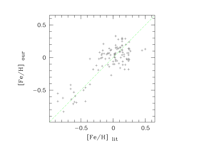
Figure 2: Comparison of our derived metallicities of Es with values from the literature (see Table Uncovering the formation of ultra-compact dwarf galaxies by multivariate statistical analysis)

Integrated colors not only depend on both mean metallicity and age of a galaxy, but may also be affected by internal extinction, possible ionized gas emission near the galactic center, etc. There is a large number of unknown parameters. To model the influence of age and metallicity on integrated colors, we use the fundamental luminosity-metallicity relation common for dwarf and giant ellipticals (Prugniel et al., 1993; Thomas et al., 2003). We used the results of simulations of a galaxy with exponentially declining star burst to derive the approximate dependence of the broad-band colors on $M/L_{V}$, age, and $[Fe/H]$ (Bell & de Jong, 2001; Matkovic & Guzman, 2005). We selected colors more sensitive to age or to metallicity. $I-K$ shows a minimal dependence on age and $M/L_{V}$. There is a strong correlation between $B-R$ and stellar M/L ratio independent of metallicity or star formation rate (Bell & de Jong, 2001). $U-B$ is very sensitive to the age of a stellar system and its M/L ratio. The slope of the color-magnitude relation, and the color – velocity dispersion ($\sigma$) relation mainly depend on metallicity. Since mass is correlated with $\sigma$ for Es, the color – velocity dispersion ($\sigma$) relation is equivalent to the mass metallicity relation. The age difference between galaxies contributes mainly to the scatter of the mass-metallicity relation. Fig.2 compares our metallicity estimates for 105 ellipticals of our sample with values from the literature.

Table 1 summarizes the data described in Sec. 2. The successive columns give : name, log$R_{h}$ ($R_{h}$ in pc), $M_{K}$, $\mu_{h,K}$, $M_{vir}/L_{K}$, $M/L_{V}$, the broad-band colors (U - B), (B -V), (V - I) and (B - K), the metallicity ($[Fe/H]$) and age determined by us, the metallicity and age from the literature, the reference to the latter two data, and finally the group. Our main contribution to the data is to have derived ages and metallicities for 26 GCs in M31, ages and metallicities for Es, and stellar mass-to-light ratios for most objects of the sample.

3 The K-Means clustering technique

Cluster analysis (CA) is the art of finding groups in data. Over the last forty years different algorithms and softwares have been developed for CA. The choice of a clustering algorithm depends both on the type of data available and on the particular purpose.

In the present study we have used the K-Means partitioning algorithm (MacQueen, 1967) for clustering. This algorithm constructs K clusters i.e. it classifies the data into K groups which together satisfy the requirement of a partition such that each group must contain at least one object and each object must belong to exactly one group. So there are at most as many groups as there are objects ($K\leq n$). Two different clusters cannot have an object in common and the K groups together add up to the full data set. Partitioning methods are applied if one wants to classify the objects into K clusters where K is fixed (which should be selected optimally). The aim is usually to uncover a structure that is already present in the data. K-Means is probably the most widely applied partitioning clustering technique.

To perform K-Means clustering we used the MINITAB package. The K-means clustering technique depends on the choice of initial cluster centers. But this effect can be minimized if one chooses the cluster centers through group average method (Milligan, 1980). As a result, the formation of the final groups will not depend heavily on the initial choice and hence will remain almost the same according to physical properties irrespective of initial centers.

With this algorithm we first determine the structures of sub populations (clusters) for varying numbers of clusters taking K = 2, 3, 4, etc. Then using the Gap Statistics (see below) we determine the optimum number of groups.

3.1 The Gap Statistics

In order to find the optimum number of groups we follow the algorithm of Gap Statistics (Tibshirani et al., 2001). Suppose that a data set ${y_{il}}$, i = 1, 2, …, n, l = 1, 2, …, p, consists of p features measured on n independent observations. Let $d_{ij}$ denote the distance between observations i and j. The squared Euclidean distance $\sum_{l}$$(y_{il}-y_{jl})^{2}$ is used as a most common choice for $d_{ij}$. Suppose that the data have been grouped into k groups G1, G2, …, Gk, with Gr denoting the indices of observations in group r, and $n_{r}$ is the number of observations in group r. Let

$$D_{r}=\sum_{i,j\in G_{r}}d_{ij}$$ (3)

be the sum of the pairwise distances for all points in cluster r, and let

$$W_{k}=\sum\frac{1}{2n}D_{r}$$ (4)

In the case that $d$ is the squared Euclidean distance, $W_{k}$ will be the pooled within-cluster sum of squares. The graph of $log(W_{{}_{k}})$ is standardized by comparing it with its expectation under an appropriate null reference distribution of the data. The estimate of the optimal number of clusters is then the value of k for which $log(W_{k})$ falls the farthest below this reference curve. Hence the gap is defined by

$$Gap_{n}(k)=E^{*}_{n}{log(W_{k})}-log(W_{k})$$ (5)

where $E^{*}_{n}$ denotes the expectation from the reference distribution. The estimate $\kappa$ will be the value maximizing $Gap_{n}(k)$ on the basis of the corresponding sampling distribution. As a motivation for the Gap Statistics, one may consider clustering n uniform data points in p dimensions, with k centers. Then assuming that the centers align themselves in an equally spaced fashion, the expectation of $log(W_{k})$ is approximately

$$log(pn/12)-(2/p)log(k)+constant$$ (6)

In other words, the Gap Statistics is defined as the difference between the log of the Residual Orthogonal Sum of Squared Distances (denoted $log(W_{k})$) and its expected value derived using bootstrapping under the null hypothesis that there is only one cluster. In this implementation, the reference distribution used for the bootstrapping is a random uniform hypercube, transformed by the principal components of the underlying data set. If the data actually have K well-separated clusters, then it is expected that $log(W_{k})$ will decrease faster than its expected rate (2/p)log(k) for $k\leq K$. When $k\succ K$, then a cluster center is essentially added in the middle of an approximately uniform cloud and simple algebra shows that $log(W_{k})$ should decrease more slowly than its expected rate. Hence the Gap Statistics should be largest when k = K.

3.2 The algorithm to find the Gap Statistics

Two common choices for the reference distribution are : (a) each reference feature is generated uniformly over the range of the observed values for that feature; (b) the reference features are generated from a uniform distribution over a box aligned with the principal components of the data.

In other words, if X is an n$\times$p data matrix, it is assumed that the columns have mean 0 and then the singular value decomposition X = UD$V^{T}$ is performed. It is transformed through Y = XV and then uniform features, say T, are drawn over the ranges of the columns of Y, as in method (a) above. Finally it is back-transformed via Z = T$V^{T}$ to give reference data, say Z. Method (a) has the advantage of simplicity. Method (b) takes into account the shape of the data distribution and makes rotationally invariant, as long as the clustering method itself is invariant.

In each case, $E^{*}_{n}{log(W_{k})}$ is estimated by an average of B copies $log(W^{*}_{k})$, each of which is computed from a Monte Carlo sample $Y^{*}_{1},Y^{*}_{2},...,Y^{*}_{n}$ drawn from the chosen reference distribution. Finally, one needs to access the sampling distribution of the Gap Statistics. Let $s_{d}(k)$ denote the standard deviation of the B Monte Carlo replicates $log(W^{*}_{k})$. Accounting additionally for the simulation error in $E^{*}_{n}{log(W_{k})}$ results in the quantity $s_{k}$ = $\sqrt{(1+1/B)}s_{d}(k)$. Using this the estimated cluster size $\kappa$ is chosen to be the smallest k such that $Gap(k)\geq Gap(k+1)-s_{k+1}$. where $s_{k+1}$ is a function of standard deviation of the bootstrapped estimates.

The computation of the Gap Statistics proceeds as follows:

• Step 1: The observed data is clustered by varying the total number of clusters from k= 1, 2, …, K, giving within-dispersion measures $W_{k}$, k = 1, 2, …, K.

• Step 2: B reference data sets are generated using the uniform prescription (a) or (b) above and each one is clustered giving within-dispersion measures $W^{*}_{kb}$, b = 1, 2, …, B, k = 1, 2, …, K. Then the estimated Gap Statistics is calculated as follows: Gap(k) = $(1/B)\sum_{b}log(W^{*}_{kb})$-$log(W_{k})$.

• Step 3. Let $\bar{l}=(1/B)\sum_{b}log(W^{*}_{kb})$, then the standard deviation is computed as

  $sd_{k}$=$[(1/B)\sum_{b}{log(W^{*}_{kb})-\bar{l}}^{2}]^{\frac{1}{2}}$

  and $s_{k}$ is defined as $s_{k}$=$sd_{k}\sqrt{(1+1/B)}$.

Finally that number of clusters are chosen such that $\kappa$=smallest k and

$$Gap(k)\geq Gap(k+1)-s_{k+1}$$ (7)

In other words the optimum number of clusters is that k for which the difference

$$u_{k}=Gap(k)-(Gap(k+1)-s_{k+1})\geq 0$$ (8)

4 Results

The parameter set chosen for CA consists of $M_{K},log(\sigma_{0}),logR_{h},M_{vir}/L_{K},[Fe/H],M/L_{V}$. Parameters like $M_{vir}$, $\mu_{h,K}$ and age are not used. $M_{K}$

is very highly correlated with $M_{vir}$ and $\mu_{h,K}$, so inclusion of these parameters does not influence the clustering. Age is excluded because of the large uncertainties associated to it. The remaining parameters are not used because of the large number of missing values. But, once the substructures are identified, all the parameters are used to identify the distinctive properties of the groups.

We have calculated the Gap Statistics for the set of six above parameters, and the output suggests that the optimum number of clusters is either four or six because the criterion used in Gap Statistics to find the optimal number of clusters, i.e. $u_{k}=Gap(k)-(Gap(k+1)-s_{k+1})\geq 0$ is satisfied for k = 4 and k = 6. Table 2 and Fig.3 show that the value of $u_{k}$ exceeds 0 for k = 4 and k = 6 and there is a sharp decline of the graph after the value k = 6. Hence, considering all the criteria discussed above, the optimal number of clusters for the present sample is k = K = 6. The six clusters (hereafter named groups to avoid confusion with star clusters) are designated FK1 to FK6, and their average properties are given in Table 2.

The elliptical galaxies were divided into two groups by the CA: high-mass ellipticals (gEs) in FK1 and low-mass ones (dEs) in FK5. Note that the labels “gE” and “dE” do not refer strictly to the morphological types commonly used in astronomy. We use these designations conditionally, to stress the statistical difference in mass between the objects of FK1 and FK5.

FK3 has the high-metallicity GCs and the bright and high-metallicity IMOs. The brightest IMOs are UCD2 ($M_{K}=-16.32$), VUCD3 ($M_{K}=-16.21$), and UCD3 ($M_{K}=-16.215$) (Hilker et al., 2007; Evstigneeva et al., 2007).

FK6 is composed of IMOs, of the most massive GCs in the Galaxy, in M31, and in NGC5128, (these GCs are all of low metallicity), and of dSphs of the Local group : Leo I (Dist.$=0.25$ Mpc) and Sculptor (Dist.$=0.08$ Mpc).

Two groups, FK2 and FK4, have a negligibly small number of members compared to the other groups : they contain three members each. These are Local Group dSphs, listed according to their distances from the Sun in Mpc: UMi (FK2, 0.066), Draco (FK2, 0.086), Sextans (FK2, 0.086), Carina (FK4, 0.1), Fornax (FK4, 0.14), Leo II (FK4, 0.21). We unfortunately do not have the full set of parameters for the other dSphs in the Local Group and nearby groups to include them in the analysis. A probable reason why these six objects were classified in such a way is their M/L ratio, which is higher than for the other galaxies. These two groups are considered only briefly, as their study is the subject of a separate and elaborate study. So there are essentially four groups found as a result of our cluster analysis.

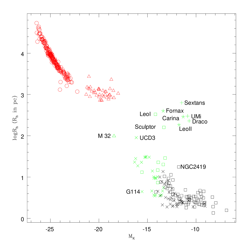
Figure 4: Absolute K magnitude versus logarithm of effective radius. The elliptical galaxies are in red, the IMOs are in green and the GCs are in black. Open circles are for FK1, pluses are for FK2, crosses are for FK3, asterisks are for FK4, triangles are for FK5 and open squares are for FK6.

We show in Fig.4 how the various types of objects are distributed among the different groups in $M_{K}$ - log$R_{h}$ space. The six groups are indicated by different symbols, colored according to the morphological type of the objects: GCs in black, IMOs in green, and ellipticals in red.

To justify our choice of sample, and to show that it is representative of stellar systems in the local Universe, we compare it to that of (Misgeld & Hilker, 2011), (hereafter MH2011) who, like us and F08, studied a sample of stellar systems covering a large range in masses, sizes and luminosities.

The sample of MH2011 is larger than ours, but the associated data do not include velocity dispersions, metallicities or ages, so we could not perform a similar analysis with their data. Nevertheless, our sample covers basically the same space in absolute magnitudes and effective radii, as shown in Fig.4, which can be compared to Fig.1 of MH2011. The main difference is that the sample of MH2011 has many more dEs (in the Hydra I and Centaurus clusters of galaxies), and extragalactic GCs (mostly GC candidates in Virgo) and they included much fainter dwarf galaxies of the Local Group, for which velocity dispersions would be very difficult to measure. In short, our sample does not appear to be biased against any particular type of object.

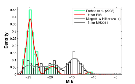
Figure 5: Probability density functions of absolute K magnitude $M_{K}$. They are plotted in green for our sample and in black for MH2011. The lines are non-parametric density approximations. They are in red for our sample and in gray for MH2011.

We also computed the probability density distribution (PDF) of $M_{K}$ in our sample and compared it to the same distribution for the MH2011 sample (see Fig.5). The method of non-parametric density estimates is described in a previous paper (Chattopadhyay et al., 2009). The bin width for computing the density estimates is the same as for the histograms shown in Fig.5. Since MH2011 gives $M_{V}$ rather than $M_{K}$, we simply shifted their V magnitudes by 2.90, which is the average value of (V - K) in our sample. There are three main populations in both samples, the faintest one being much more important in MH2011. Anticipating on our results, we expect the distribution of metallicities for the F08 and MH2011 samples to be similar due to the fact that Es follow the fundamental luminosity-metallicity relation (Prugniel et al., 1993; Thomas et al., 2003).

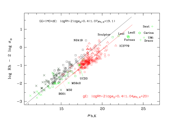
Figure 7: Edge-on projection of the Fundamental Plane for the six groups. The symbols and colors are the same as in Fig.4.

The successive peaks are at $M_{K}$ = -24.8, -19.7, -13.3, -11 in our sample, and at $M_{K}$ = -25, -19.4, -14.8 in the sample of MH2011. The first peak in both samples corresponds to bulges and the brightest elliptical galaxies. The next peak appears at the location where the linear size - luminosity relation, common for ellipticals and UCDs (MH2011), splits into two : one relation for dwarf galaxies and one for compact ellipticals and GCs. This occurs at about $R_{h}$ = 1.3 kpc and $Mass=10^{10}M_{\odot}$. So, galaxies in this group have roughly constant effective radii. The faintest objects in this group have luminosities similar to M32, $M_{K}\sim 18.5$, but their stellar densities are two orders of magnitude lower (see Fig.5 in MH2011). The highest stellar density for this group may be a characteristic scale, dividing stellar systems into two systems. The internal acceleration for one group is within the limits postulated in MONDian dynamics, while for the other groups it is outside those limits. See also the caption of Fig.7 of MH2011. The faintest broad PDF peaks (-13.3 and -11 in our sample and -14.8 in MH2011) are different for both samples. However, this is just a selection effect : as mentioned above, our sample contains fewer dEs.

So, again, our sample does not differ significantly from another large sample of stellar systems. Our sample does not reflect the local luminosity function for individual types of objects, and neither does the sample of MH2011. We suggest that the relative intensity of the PDF peaks in both samples reflects the way in which the samples were selected.

We also examined whether our choice of objects in the F08 sample (370 out of 499) could bias the results in some way. We have computed the mean $\pm$ standard error values of $M_{K}$ and $log(\sigma_{0})$ in the sub samples 1, 2, and 3 considered by F08 as well as for our corresponding sub samples. The number of objects is of course different in the present sample and in the F08 sample. But from Table 4 it is quite clear that this feature does not introduce any significant bias as the mean values are very similar.

We now present the distinctive properties of the groups, and look for possible physical reasons for the differences and similarities between the groups.

5 Properties of the groups

5.1 Mass-to-luminosity ratios and binding energies

We will discuss the virial M/L ratio, and it is important for what follows to keep in mind that the stellar $M/L_{V}$ derived using photometric data and SSP models is not necessarily identical to the true baryonic M/L. This is due to the difficulty to correctly take into account the star formation history (SFH) and initial mass function of stellar populations (e.g. Trager et al., 2008, MH2011). Furthermore, a disagreement between virial and baryonic M/L may be due to the presence of dark matter, if the stellar population model including SFH and initial mass function is correct.

The difference between virial and stellar M/L for our sample can be seen from Table 1. It is seen that both the virial ($M_{vir}/L_{K}$) and the baryonic ($M/L_{V}$) mass-to-light ratios differ at a high level of significance among the four main groups. Hereafter we will concentrate on $M_{vir}/L_{K}$ and simply call it M/L. It is well known that UCDs tend to have higher M/L than GCs (Dabringhausen et al., 2008, F08), and that dwarf spheroidal galaxies have very high M/L from direct radial velocity measurements of their brightest stars (e.g. Simon & Geha, 2007). Additionally, UCDs, like galaxies, have relaxation times greater than the Hubble time (Kroupa, 1998). This is usually demonstrated by plotting the data in the $k_{1}-k_{3}$ space introduced by Bender et al. (1992), and this is well discussed in the aforementioned papers.

For the present data, these parameters are :

$$k_{1}=(log\sigma_{0}^{2}+logR_{h})/\sqrt{2}$$

$$k_{2}=(log\sigma_{0}^{2}+2logI_{e}-logR_{h})/\sqrt{6}$$

and

$$k_{3}=(log\sigma_{0}^{2}-logI_{e}-logR_{h})/\sqrt{3}$$

where $I_{e}$ is given by Eq. 1. These coordinates are simply related to physical quantities : $k_{1}$ is proportional to the logarithm of mass, $k_{2}$ is proportional to the effective surface brightness times M/L, and $k_{3}$ is proportional to the logarithm of M/L.

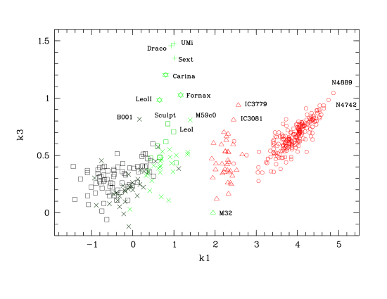
Figure 6: Projection of the FP for dynamically hot stellar systems. $k_{1}$ and $k_{3}$ are related to mass and M/L respectively. The symbols and colors are the same as in Fig.4.

The differences in mass (represented by $k_{1}$) and M/L (represented by $k_{3}$) between the groups are shown in Fig.6. The groups occupy different locations in this projection of the FP, except FK3 and FK6. For these two groups there is no continuity break in the $k_{1}$, $k_{3}$ parameter distributions as for other groups. Both FK3 and FK6 contain objects with high M/L. FK3 includes IMOs, and FK6 contains dSphs (Sculptor and Leo I) and IMOs. We also note that the four main groups show wide and different ranges in both mass and M/L. In each group, more massive objects show higher M/L, but the slope of the correlation is different for each group.

To quantify this, we performed robust multilinear regressions of the form $k_{3}=a+bk_{1}$ on the four main groups. The resulting fits are listed in Table 5. The regression lines for the groups FK3, FK5, and FK6 correspond to the relation M/L$\propto$ M^0.2 within the errors. M/L is proportional to M^0.31 for the group FK1. The position of the different objects within the groups on the FP reflects not only differences in M/L, but also in surface density, luminosity, and kinematical structure (Djorgovski & Davis, 1987). According to the slopes of the relations, the objects in FK1 are much more influenced by the above three factors than the objects in FK3, FK5 and FK6.

We now move on to discuss the edge-on projection of the Fundamental Plane (Djorgovski & Davis, 1987; Faber & Jackson, 1976; Kormendy, 1977; Djorgovski, 1995) shown in Fig.7. This figure is a representation of the Virial Theorem: $r_{e}\propto\sigma_{0}^{2}I_{e}^{-1}(M/L)^{-1}$, usually applied to galaxies (Faber et al., 1989; Djorgovski et al., 1989). This figure also serves to compare the binding energies of GCs (McLaughlin, 2000). The most compact and luminous GCs have larger binding energies.

The groups FK3, FK5, and FK6 (i.e. GCs, IMOs and dEs) follow roughly the same relation in the edge-on projection of the FP (Fig.7). We obtained a bivariate least squares solution fitted through $\mu_{h,K}$:

$$logR_{h}-2log\sigma_{0}=0.4(1.07(\pm 0.03)\mu_{h,K}+19.1(\pm 0.1))$$

which corresponds to $r_{e}\propto\sigma_{0}^{2}I_{e}^{-1.1}.$ The gEs of FK1 are concentrated in a parallel sequence, shifted towards lower surface brightnesses ($\mu_{h,K}$). The bivariate correlation for FK1 gives:

$$logR_{h}-2log\sigma_{0}=0.4(1.04(\pm 0.06)\mu_{h,K}+20.0(\pm 0.13))$$

These two solutions are close to the one that satisfies the Virial Theorem. The different slope (1.07 in the first case, 1.04 in the second) is referred to as the tilt in the FP, whose cause is still under debate (see Fraix-Burnet et al., 2010, and references therein). The tilt of the virial mass - total stellar mass relation common for gEs, cEs and UCDs/GCs has been discussed in F08. The difference in the zero points includes three components (e.g. Kormendy, 1989, and references therein). The first one reflects the density, luminosity and kinematic structure of objects. The second factor indicates whether the system is gravitationally bound or virialized. If the deviation from the FP is due to mass-to-light ratio, this implies the scaling relation $M/L\propto M^{0.2}$. The systematic shift between gEs and the groups of GCs, IMOs, and dEs is mainly due to the approximately ten times larger M/L for gEs (Dabringhausen et al., 2008).

The objects of FK3 and FK6 are well mixed together in Fig.7, with a tendency for FK3, which contains IMOs, to have higher binding energy. The objects with the strongest deviation from the relation are IMOs: e.g. B001, M59cO, UCD3; the globular cluster NGC2419, and some dEs, like IC3779, with $\mu_{h,K}>20$ mag arcsec^-2. M32 has a very high binding energy, similar to that of IMOs. Some gEs also fall in the same region of the diagram, as M32, but no other dE does. Bekki et al. (2001) and Graham (2002) argued that M32 is the stripped core of a larger galaxy. NCG2419 shows a lower binding energy than other GCs. Dabringhausen et al. (2008) considered it as the most likely candidate to host dark matter.

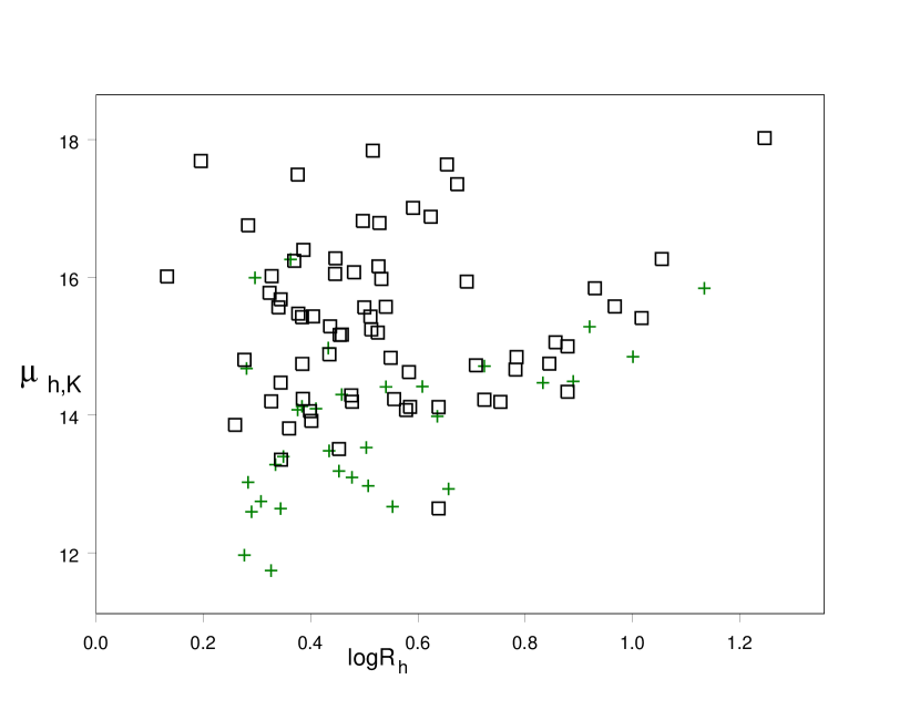
Figure 8: The surface brightness ($\mu_{h,K}$) versus half light radius ($logR_{h}$) profile for GCs in groups FK3 (green, plus) and FK6 (black,box) respectively.

The $\mu_{h,K}$ versus $logR_{h}$ diagram (Fig.8) illustrates the difference in stellar densities between the GCs of FK3 and FK6. It shows that the GCs in FK3 have higher $\mu_{h,K}$ than those in FK6 at a given $R_{h}$. In other words, FK6 has statistically shallower surface brightness profiles than FK3. On the other hand, the IMOs and GCs in FK3 are more massive/luminous and compact in general than those in FK6. Jordán et al. (2005) found a significant correlation between half-light radius and color for early-type galaxies in the Virgo cluster in the sense that the red GCs are smaller than the blue ones.

Having studied how mass is related to luminosity in our different groups, we now examine how mass is related to metallicity.

5.2 Mass-metallicity relation

It is now well established that more massive galaxies are also more metal rich; this is a consequence of the hierarchical formation of galaxies in the Universe. But does such a relation hold for all types of stellar systems?

5.2.1 A boundary line

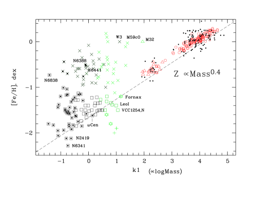
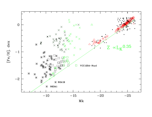
Figure 9: $k_{1}$ versus $[Fe/H]$ (a) and $M_{k}$ versus $[Fe/H]$ (b) for the six groups. The symbols and colors are the same as in Fig.4. Black dots for ellipticals indicate metallicities from the literature. Black dots for GCs (open squares) indicate Galactic GCs

The mass-metallicity relation (hereafter MMR) for our sample objects is shown in Fig.9a, where $k_{1}$, which is equivalent to mass, is plotted versus $[Fe/H]$.

This figure shows that, except for a few objects, all types of stellar systems lie above a boundary line. It was plotted to stress the tendency, but its slope is surprisingly close to a MMR of the form $Z\propto Mass^{0.4}$. The correlation is very weak for the objects in FK3 ($r(M_{K},[Fe/H])=-0.382$) and FK6 ($r(M_{K},[Fe/H])=-0.177$), if we consider them globally. Only the brightest low-metallicity GCs (FK6) and IMOs at a given metallicity are close to the MMR. The picture is almost the same if we plot absolute K magnitude versus $[Fe/H]$ (Fig.9b). However, here the slope of the boundary line is slightly different from that of the MMR: $[Z/H]\sim-3.5-0.14M_{K}$.

What could be the origin of the boundary line? It is unlikely to be caused by an observational selection effect. We would presumably not see it if we included in the sample only high-metallicity GCs and galaxies of other morphological types. Many of the GCs are the brightest GCs of our Galaxy, and their metallicities are very accurate. Extragalactic GCs and IMOs are also bright. Their metallicities were obtained mainly via spectroscopy, and are not very much influenced by observational errors and the age-metallicity degeneracy. The only really uncertain metallicities are those of ellipticals, because of the age-metallicity degeneracy and uncertainties due to possible internal extinction, light-element abundance variations, and large age and metallicity spreads within individual galaxies. But, in spite of these uncertainties, the ellipticals do follow the relation.

The slope of the boundary line is similar to that of the luminosity-metallicity relation found in the literature. A luminosity-metallicity relation, $[Z/H]=-3.6-0.19M_{B}$, was found for dwarf and giant ellipticals in nearby galaxy clusters by Thomas et al. (2003). It is equivalent to the equation $Z\propto L^{0.4}$, found for dwarf galaxies in the Local Group by Dekel & Silk (1986), since $[Z/H]=[Fe/H]+0.94[\alpha/Fe]$ (Thomas et al., 2003), $log(L_{B}/L_{\odot})=0.4(5.48-M_{B})$, and $logZ\sim 0.977[Fe/H]-1.699$ (Bertelli et al., 1994). We used here the solar value $[\alpha/Fe]=0$. However, the deviations from this relation for massive ellipticals may be large due to strong variations in $[\alpha/Fe]$ for Es: $\sim 0.2\div 0.5$ dex (Thomas et al., 2003; Puzia et al., 2006, and references therein). The median of the metallicity distribution for elliptical galaxies and galactic bulges from the Sloan Digital Sky Survey obtained by Gallazzi et al. (2005) as a function of stellar mass is also close to the relation $Z\propto M^{0.4}$ (see also Dabringhausen et al., 2008).

The origin of the luminosity-metallicity and mass-metallicity relations for different morphological types of galaxies is still an open issue (e.g. Grebel et al., 2003; Finlator & Dave, 2008; Kunth & Ostlin, 2000). Does star formation define the shape of the MMR? Does the boundary line mean a lower fraction of matter capable of being transformed into stars under special physical conditions? It might result from the interplay between internal and environmental factors: mergers and interactions, inflows and outflows of gas, star formation histories of individual galaxies in hierarchical galaxy formation.

The luminosity-metallicity relation for brightest GCs has been extensively studied (Harris et al., 2006; Mieske et al., 2006; Peng et al., 2009). Using linear color-metallicity relations for blue GCs, these studies derive scaling relations between GC luminosity L and metallicity Z consistent with $Z\propto L^{0.5}$ (e.g. Strader & Smith, 2008). The slope depends on the SSP models and on the light-element abundances. According to Carney (1996) the mean $[\alpha/Fe]$ for Galactic GCs is 0.3 dex. The same value was used by Dabringhausen et al. (2008) to calculate $[Z/H]$ for IMOs.

The metallicity of the faintest GCs close to the MMR is intriguing. It corresponds approximately to extreme abundances of Population II stars, i.e. stars formed immediately after the initial pollution of interstellar medium by massive Population III stars: $Z\sim 0.01Z_{\odot}$ (Silk, 1985).

The Color-magnitude diagram (CMD) and chemical composition of some GCs located near the border line (i.e. $\Omega$Cen, NGC2419, NGC 6341) are unusual. For example, NGC2419 is considered a remnant of a dwarf galaxy due to its peculiar chemical composition (Cohen et al., 2010). The CMDs of most of these GCs show the existence of multiple stellar populations, a fact that is still not fully understood (see e.g. Bedin et al., 2008; Marin-Franch et al., 2009; Renzini, 2008, and references therein). Since these GCs and IMOs are close to the MMR, they were probably the brightest parts (nuclei) of tidally destructed host galaxies (Zinnecker et al., 1988; Bekki et al., 2003). They may also be geniune compact dwarf galaxies originating from small-scale peaks in the primordial dark matter power spectrum (Drinkwater et al., 2004). GCs may have formed in dark matter minihaloes (Mashchenko et al., 2005). However, it has not been established whether they actually contain dark matter haloes (Jordi et al., 2009; Baumgardt et al., 2009).

The Local Group dSphs and some GCs definitely fall below the border line in the $k1$ versus $[Fe/H]$ diagram. The reason has been studied extensively for dSphs. Dwarf galaxies with luminosities below some limit lose gas effectively because of their low gravitational potentials, too shallow to prevent stellar outflows following star formation episodes (e.g. Dekel & Silk, 1986; Grebel et al., 2003).

5.2.2 Metallicity bimodality

There is a gap between the groups FK6 and FK3 in Figs.9(a, b). It is located near $[Fe/H]=-1.0$ and is not horizontal. The low-metallicity peak is near $[Fe/H]=-1.6\pm 0.4$ dex, the high-metallicity one is near $[Fe/H]=-0.6\pm 0.04$ dex. Similar metallicity peaks and the dividing line were identified for the GC system of our Galaxy by (Harris, 1989). GC systems of massive Es and many spirals follow a bimodal color distribution (Harris et al., 1996; Gebhardt & Kissler-Patig, 1999; Larsen et al., 2001; Peng et al., 2006). A new feature shown in Fig.9 is that the metallicity distributions of IMOs and extragalactic GCs fall in the same range as the GCs of our Galaxy. Extragalactic objects are gathered in two homogeneous groups together with Galactic GCs.

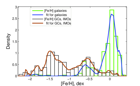
Figure 10: Probability density functions of metallicity $[Fe/H]$. They are plotted in green for galaxies and in black for GCs and IMOs. The lines are non-parametric density approximations. They are in blue for galaxies and in brown for GCs and IMOs.

Fig.10 shows the probability density distribution of $[Fe/H]$ for all galaxies (FK1 + FK5 + FK4 + FK2), and for GCs and UCDs (FK6 + FK3). The distribution is computed in the same way as the PDF shown in Fig.5. Although the groups are not plotted with different colors, they are clearly distinguishable from the PDF peaks. The local maximum in the distribution for group FK3 at $[Fe/H]\sim-0.6$ is close to that of FK5 (”dEs”), which is composed of galaxies having a roughly constant effective radius and departing from the size - mass relation common for gEs and UCDs (MH2011). The corresponding PDF peak is also present in the probability density distribution of luminosities (see discussion at the end of Sec.4). The PDF for group FK6 corresponds to that of groups FK2+4, i.e. galaxies less massive than 10⁸ stellar masses. Interestingly, there is another gap at the level of $[Fe/H]\sim-0.3$, between six IMOs (M59cO, W3, W30, G114, VUCD 3, S490) and the other objects in FK3. M32 with a central velocity dispersion of $\sigma_{0}\sim 79$ km/s also falls in this metallicity range. However, since the luminosity and metallicity distributions of galaxies are influenced by sample selection effect, the correlation is not sufficient to establish the tidal origin of nuclear GCs and UCDs.

The nature of the bimodality in the metallicity distribution is a complex, still unanswered question. Due to the stochastic nature of galaxy formation and star formation, hierarchical scenarios do not reproduce the metallicity bimodality well. The dependence of the galactic SFH on stellar mass is not straightforward (Thomas et al., 2005; Renzini, 2009). Additionally, there is a strong morphology-density relation, the environmental dependence between stellar mass, structure, star formation and nuclear activity in galaxies (e.g. Kauffmann et al., 2004; Renzini, 2006). Recent spectroscopic studies have revealed strong age and metallicity gradients of different slopes and values between the nuclear and outer regions of elliptical galaxies (Koleva et al., 2011, and references therein). Nuclear activity in galaxies often continues longer than in the outer regions, because the fuel for star formation falls towards the gravitational center. So, nuclei may contain multiple stellar populations, and be on average younger and more metal-rich than the rest of the galaxy. There are anomalous objects in both FK3 and FK6. In the low-metallicity group GCs like $\Omega$Cen, NGC2419 and NGC 6341 show evidence of multiple stellar populations. The metal-rich GCs NGC6441 and NGC6338 have prominent blue extensions in the horizontal branch (Rich et al., 1997), which are not typically associated with a globular cluster of this metallicity, like 47 Tuc.

It has been proposed that the outer-halo GCs of the Galaxy were accreted from the satellite galaxies (e.g. Mackey & Gilmore, 2004; Chattopadhyay & Chattopadhyay, 2007; Chattopadhyay et al., 2007; Mondal et al., 2008). Shapiro et al. (2010) suggest that high-metallicity old GCs were formed from super star-forming clumps with radii 1-3 kpc and masses $10^{8}$ to $10^{9}M_{\odot}$, which are known as a key component of star-forming galaxies at $z\sim 2$.

5.2.3 Efficiency of metal production

Is there a similar physical quantity for dynamically hot stellar systems lying close to the MMR? For young stellar systems, for example, the star formation rate is known to be an important factor influencing the MMR (Mannucci et al., 2010, and references therein). In Fig.11 we plot the dependence of $[Fe/H]$ on the metallicity per unit effective luminosity density in the K band. We call the last term ”metal production efficiency” (MPE) by analogy with the star formation efficiency (SFE), which is the fraction of gas converted into stars at a particular evolutionary stage of galaxies (Kennicutt, 1998). MPE also reflects the stellar density and the size of dynamically hot stellar systems. Fig.11 shows that GCs and UCDs in FK6 have MPE in the same range as Es: gEs (FK1) (MPE$=2.7\pm 0.25$), and dEs (FK5) (MPE$=1.7\pm 0.4$). Galaxies with stellar masses $M<10^{10}M_{\odot}$, including dSphs and GCs + UCDs (FK3+FK6), are in two separate sequences, both showing a tendency for metallicity to increase linearly with MPE. The two sequences intersect at the location of the brightest UCDs and M32-like objects. Fig.11 also shows that the objects of FK3 are the most metal-rich per unit effective luminosity density. So, at least for these GCs and UCDs in our sample, it is reasonable to assume that they are the densest parts of galaxies accumulating fuel for star formation.

6 Conclusion

A multivariate statistical technique, K-Means clustering, has been carried out on a data set taken from the paper of Forbes et al. (2008). It consists of elliptical galaxies, intermediate mass objects, Local Group dwarf spheroidals, nuclei of dwarf ellipticals, young massive objects and globular clusters. The sample properties were completed by data from the literature or derived by us. Our aim was to investigate the existence of interconnectedness, if any, among the six groups found by our multivariate analysis.

In order to inquire into the physical origin of IMOs, we considered different projections of the fundamental plane using the results of the statistical analysis along with observational data on velocity dispersion, effective radii and effective surface brightness calculated from the total absolute magnitude in the K band. We found that our groups are different in terms of virial M/L ratios, and dependences between virial M/L ratios and mass.

The value of our study is that we include metallicities along with other data in addition to the list of parameters of F08, which definitely helps us to provide an objective classification into groups. We consider a unified mass-metallicity dependence for all the sample objects. It shows that (i) there are GCs and UCDs in the low-metallicity group sharing MMR with galaxies; (ii) there are signatures of bimodality/multimodality in the metallicity distribution that are common for GCs and IMOs on one hand, and for low- and high-mass Es on the other hand. We speculate that the rate of SF at the epoch when the objects were young is the probable reason for the above two features. It appears that the mean metallicities per effective K-band luminosity density (MPE) for GCs and UCDs in FK6 lie in the same range as for elliptical galaxies, suggesting similar physical processes and SFE. However, MPE is much higher for GCs and UCDs in FK3. This confirms that these objects originated as the densest parts of the present day Es.

According to our findings, IMOs may be divided into two physical groups: (i) Dwarf galaxy - globular cluster transition objects formed in the same way and from the same material as old galaxies and (ii) nuclei stripped from dwarf and normal ellipticals during their dynamical evolution in groups and clusters. Note that since UCDs were found only in dense environments, the last suggestion is highly probable. Extensive theoretical and observational studies are needed to establish the reasons for the described features and the exact nature of UCDs.

7 Acknowledgements

T. C. thanks DST, India for supporting her a Major Research Grant. M. S. acknowledges partial support of grants GK. 14.740.11.0901, RFBR 11-02-90449 UKR-f-a, RFBG 11-02-00639-a, and thanks IRAP for its hospitality. We thank the anonymous referee for detailed comments which helped to improve the paper.

Figure 1: Effective radius $R_{h}$ computed by us (filled circles) and $R_{20}$ from F08 (crosses) versus absolute K magnitude $M_{K}$. This figure is to be compared to Fig.3 of F08.

epsscale2.0

Figure 3: The gap curve.

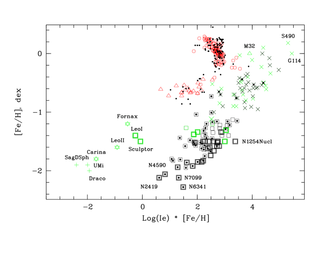
Figure 11: $[Fe/H]$ versus metallicity per unit effective luminosity density. The symbols and colors are the same as in Fig.9. Bold symbols indicate that GCs and IMOs tend to follow the mass-metallicity relation.

Table 1: Photometric and structural parameters.

Name	logRh	MK	$\mu_{h,K}$	Mvir/LK	M/LV	(U-B)	(B-V)	(V-I)	(B-K)	[Fe/H]	Age	[Fe/H]lit	Agelit	Ref	Group
	(pc)	(mag)	(mag/arcsec2)	(M⊙/LK,⊙)	(M⊙/LV,⊙)	(mag)	(mag)	(mag)	(mag)		(Gyr)		Gyr
NGC104	0.60830	-12.19	14.41	0.851	2.70	0.33	0.84	1.09	3.63	$\cdots$	$\cdots$	-0.76	10.864	9,10	3
NGC1851	0.25891	-11.01	13.86	0.931	6.36	0.15	0.74	0.98	3.42	$\cdots$	$\cdots$	-1.22	8.96	9,10	6
NGC1904	0.48076	-9.90	16.07	1.074	1.85	0.05	0.64	0.90	2.68	$\cdots$	$\cdots$	-1.57	10.08	9,10	6
NGC3201	0.59083	-9.51	17.01	1.973	1.80	0.12	0.73	0.91	2.85	$\cdots$	$\cdots$	-1.58	8.624	9,10	6
NGC362	0.32645	-11.00	14.20	0.414	2.07	0.10	0.72	0.94	3.33	$\cdots$	$\cdots$	-1.16	18.512	9,10	6
NGC4147	0.37595	-7.95	17.49	1.266	1.85	0.09	0.57	0.76	2.37	$\cdots$	$\cdots$	-1.83	11.536	9,10	6
NGC4590	0.65406	-9.20	17.64	0.705	2.40	-0.02	0.58	0.87	2.45	$\cdots$	$\cdots$	-2.06	10.304	9,10	6
NGC5272	0.51294	-10.89	15.24	0.539	3.30	0.08	0.68	0.92	2.64	$\cdots$	$\cdots$	-1.57	8.96	9,10	6
NGC5286	0.34397	-10.82	14.47	0.797	1.85	0.01	0.64	0.86	2.92	$\cdots$	$\cdots$	-1.67	12.48	9,10	6
NGC5694	0.52631	-10.04	16.16	1.172	2.40	-0.02	0.60	0.86	2.86	$\cdots$	$\cdots$	-1.86	11.76	9,11	6
NGC5824	0.52518	-11.00	15.20	2.158	2.73	-0.03	0.62	0.87	2.81	$\cdots$	$\cdots$	-1.85	11.312	9,10	6
NGC5904	0.69110	-11.09	15.94	0.703	1.33	0.14	0.69	0.91	2.97	$\cdots$	$\cdots$	-1.27	9.296	9,10	6
NGC5946	0.34397	-9.61	15.68	0.520	1.50	-0.15	0.75	0.84	3.32	$\cdots$	$\cdots$	-1.38	10.08	9,10	6
NGC6093	0.27664	-10.15	14.80	3.031	3.12	0.01	0.66	0.86	2.63	$\cdots$	$\cdots$	-1.75	10.864	9,10	6
NGC6121	0.32705	-9.19	16.02	0.950	1.20	0.03	0.67	0.92	2.76	$\cdots$	$\cdots$	-1.2	10.192	9,10	6
NGC6171	0.67324	-9.58	17.35	1.395	3.50	0.32	0.77	1.00	3.32	$\cdots$	$\cdots$	-1.04	10.976	9,10	6
NGC6205	0.54000	-10.70	15.57	1.103	3.12	-0.04	0.66	0.83	2.66	$\cdots$	$\cdots$	-1.54	11.76	9,10	6
NGC6218	0.49715	-9.23	16.82	1.541	1.85	-0.01	0.64	0.88	2.61	$\cdots$	$\cdots$	-1.48	10.528	9,10	6
NGC6254	0.32346	-9.41	15.77	1.891	1.16	-0.08	0.62	0.83	2.63	$\cdots$	$\cdots$	-1.52	9.968	9,10	6
NGC6256	0.29623	-9.06	15.99	2.388	0.51	-0.12	0.66	0.80	3.50	$\cdots$	$\cdots$	-0.7	13.5	9,10	3
NGC6266	0.39873	-11.51	14.06	1.532	1.87	-0.01	0.72	0.93	3.18	$\cdots$	$\cdots$	-1.29	10.304	9,10	6
NGC6284	0.53191	-10.25	15.98	1.244	1.44	0.09	0.71	0.92	3.07	$\cdots$	$\cdots$	-1.32	9.632	9,10	6
NGC6293	0.37701	-9.98	15.47	1.676	1.39	-0.17	0.55	0.72	2.88	$\cdots$	$\cdots$	-1.92	13.5	9,10	6
NGC6325	0.33994	-9.71	15.56	1.156	1.50	-0.15	0.77	0.93	3.79	$\cdots$	$\cdots$	-1.17	13.5	9,10	6
NGC6341	0.40424	-10.16	15.43	0.916	1.80	-0.01	0.61	0.85	2.57	$\cdots$	$\cdots$	-2.28	12.096	9,10	6
NGC6342	0.36245	-9.12	16.26	1.311	2.57	0.26	0.80	0.94	3.62	$\cdots$	$\cdots$	-0.65	10.304	9,10	3
NGC6388	0.28980	-12.42	12.60	0.897	2.57	0.25	0.80	0.96	3.91	$\cdots$	$\cdots$	-0.5	10.8	9,11	3
NGC6397	0.13211	-8.22	16.01	1.701	1.80	-0.08	0.55	0.78	2.19	$\cdots$	$\cdots$	-1.95	11.2	9,10	6
NGC6441	0.34909	-11.92	13.40	1.484	2.57	0.28	0.80	0.97	3.22	$\cdots$	$\cdots$	-0.53	10.2	9,10	3
NGC6522	0.38385	-10.07	15.42	1.225	1.40	0.11	0.73	0.85	3.27	$\cdots$	$\cdots$	-1.44	13.5	9,10	6
NGC6535	0.19531	-6.86	17.69	1.957	0.95	-0.09	0.60	0.80	2.81	$\cdots$	$\cdots$	-1.8	10.44	9,10	6
NGC6541	0.38437	-10.75	14.74	0.982	2.73	-0.03	0.62	0.82	3.04	$\cdots$	$\cdots$	-1.83	12.72	9,10	6
NGC6558	0.51565	-8.31	17.84	1.572	3.60	0.09	0.67	0.86	2.65	$\cdots$	$\cdots$	-1.44	13.5	9,10	6
NGC6624	0.28063	-10.30	14.68	0.507	2.50	0.29	0.83	1.03	3.72	$\cdots$	$\cdots$	-0.44	10.68	9,11	3
NGC6626	0.43500	-10.86	14.88	1.091	3.30	0.01	0.68	0.86	3.48	$\cdots$	$\cdots$	-1.45	13.5	9,10	6
NGC6656	0.45406	-10.68	15.16	1.481	1.85	-0.10	0.64	0.95	2.92	$\cdots$	$\cdots$	-1.64	12.36	9,11	6
NGC6681	0.38645	-9.10	16.40	1.735	2.45	0.04	0.65	0.89	2.66	$\cdots$	$\cdots$	-1.51	10.416	9,10	6
NGC6712	0.44554	-9.75	16.05	0.781	1.87	0.03	0.72	0.95	3.10	$\cdots$	$\cdots$	-1.01	10.4	9,12	6
NGC6779	0.52818	-9.42	16.79	1.103	1.80	-0.07	0.66	0.88	2.76	$\cdots$	$\cdots$	-1.94	13.2	9,11	6
NGC6809	0.62359	-9.80	16.88	1.446	4.62	0.02	0.64	0.89	2.92	$\cdots$	$\cdots$	-1.81	11.76	9,10	6
NGC6838	0.28327	-8.23	16.75	0.621	2.70	0.35	0.84	1.02	3.55	$\cdots$	$\cdots$	-0.73	10.192	9,10	6
NGC6864	0.45804	-10.69	15.17	1.929	1.44	0.10	0.71	0.94	2.90	$\cdots$	$\cdots$	-1.16	9.98	9,12	6
NGC6934	0.44600	-9.52	16.28	1.352	3.60	0.09	0.67	0.85	2.76	$\cdots$	$\cdots$	-1.54	9.52	9,10	6
NGC7089	0.51139	-10.70	15.43	1.377	0.95	0.02	0.60	0.84	2.29	$\cdots$	$\cdots$	-1.62	10.528	9,10	6
NGC7099	0.36952	-9.18	16.24	1.879	1.85	0.00	0.57	0.82	2.32	$\cdots$	$\cdots$	-2.12	12.096	9,10	6
NGC2419	1.24613	-11.78	18.02	0.300	1.39	-0.05	0.55	0.90	2.78	$\cdots$	$\cdots$	-2.12	12	9,13	6
B001	0.43297	-10.76	14.97	10.113	2.30	$\cdots$	$\cdots$	$\cdots$	$\cdots$	0.15	0.17	$\cdots$	$\cdots$	$\cdots$	3
B006	0.54033	-11.86	14.41	1.000	2.10	$\cdots$	$\cdots$	$\cdots$	$\cdots$	-0.35	10.2	$\cdots$	$\cdots$	$\cdots$	3
B012	0.47712	-11.76	14.19	1.851	2.30	$\cdots$	$\cdots$	$\cdots$	$\cdots$	-1.66	6.8	-1.7	(14)	14	6
B020	0.43457	-12.26	13.48	0.827	2.40	$\cdots$	$\cdots$	$\cdots$	$\cdots$	-0.83	6.90	-0.9	8.6	14	3
B023	0.55267	-13.66	12.67	0.951	2.40	$\cdots$	$\cdots$	$\cdots$	$\cdots$	-0.91	14.0	-0.7	11.8	14	3
B034	0.33445	-11.96	13.28	0.696	2.10	$\cdots$	$\cdots$	$\cdots$	$\cdots$	-0.59	4.4	-0.6	(14)	14	3
B045	0.45788	-11.56	14.30	0.787	2.10	$\cdots$	$\cdots$	$\cdots$	$\cdots$	-0.76	10.0	-0.9	(14)	14	3
B163	0.47712	-12.86	13.09	0.863	2.50	$\cdots$	$\cdots$	$\cdots$	$\cdots$	-0.08	8.3	-0.1	13.5	14	3
B193	0.30750	-12.36	12.74	0.482	2.40	$\cdots$	$\cdots$	$\cdots$	$\cdots$	-0.2	9.6	-0.1	12.9	14	3
B218	0.50379	-12.56	13.53	1.121	2.20	$\cdots$	$\cdots$	$\cdots$	$\cdots$	-0.63	8.1	-0.8	8.7	14	3
B225	0.32634	-13.46	11.74	0.705	2.30	$\cdots$	$\cdots$	$\cdots$	$\cdots$	-0.35	3.70	-0.5	10.7	14	3
B232	0.38561	-11.26	14.24	1.636	2.20	$\cdots$	$\cdots$	$\cdots$	$\cdots$	-1.49	8.9	-1.9	(14)	14	6
B240	0.47567	-11.66	14.29	1.102	2.30	$\cdots$	$\cdots$	$\cdots$	$\cdots$	-1.74	1.79	-1.5	(14)	14	6
B311	0.40140	-11.66	13.91	1.451	1.80	$\cdots$	$\cdots$	$\cdots$	$\cdots$	-1.58	8.5	$\cdots$	$\cdots$	$\cdots$	6
B343	0.43616	-10.46	15.29	1.763	2.40	$\cdots$	$\cdots$	$\cdots$	$\cdots$	-1.28	1.82	$\cdots$	$\cdots$	$\cdots$	6
B373	0.28330	-11.96	13.02	0.598	1.90	$\cdots$	$\cdots$	$\cdots$	$\cdots$	-0.59	11.0	-0.5	13.7	14	3
B386	0.35984	-11.56	13.81	0.860	2.20	$\cdots$	$\cdots$	$\cdots$	$\cdots$	-1.13	9.7	-1.1	(14)	14	6
B405	0.58320	-11.86	14.62	0.607	2.50	$\cdots$	$\cdots$	$\cdots$	$\cdots$	-1.28	1.3	-1.2	(14)	14	6
B407	0.38382	-11.36	14.13	0.750	2.00	$\cdots$	$\cdots$	$\cdots$	$\cdots$	-0.65	5.10	$\cdots$	$\cdots$	$\cdots$	3
B158	0.34400	-12.65	12.64	0.970	2.10	$\cdots$	$\cdots$	$\cdots$	$\cdots$	-0.74	2.60	-0.8	9.1	14	3
B289	0.50000	-10.50	15.56	1.692	0.20	$\cdots$	$\cdots$	$\cdots$	$\cdots$	-1.5	0.81	$\cdots$	$\cdots$	$\cdots$	6
B338	0.63600	-12.77	13.98	1.734	2.30	$\cdots$	$\cdots$	$\cdots$	$\cdots$	-0.49	8.2	$\cdots$	$\cdots$	$\cdots$	3
B358	0.54900	-11.48	14.83	0.712	1.60	$\cdots$	$\cdots$	$\cdots$	$\cdots$	-1.85	10.0	$\cdots$	$\cdots$	$\cdots$	6
B379	0.37600	-11.37	14.07	0.533	2.60	$\cdots$	$\cdots$	$\cdots$	$\cdots$	-0.53	10.0	-0.4	10.5	14	3
B384	0.41000	-11.53	14.09	0.770	2.10	$\cdots$	$\cdots$	$\cdots$	$\cdots$	-0.59	10.3	-0.7	13.5	14	3
OmegaCen	0.78387	-12.64	14.84	1.631	3.12	0.06	0.66	0.88	3.05	$\cdots$	$\cdots$	-1.62	11.28	9,10	6
M54	0.58529	-12.38	14.12	1.041	3.20	0.07	0.70	0.89	3.11	$\cdots$	$\cdots$	-1.58	10.8	9,10	6
NGC2808	0.34454	-11.94	13.35	0.796	1.35	0.03	0.70	0.88	3.32	$\cdots$	$\cdots$	-1.15	8.624	9,10	6
G1	0.50709	-13.13	12.97	1.640	0.17	0.13	0.57	0.64	3.51	-0.73	9	$\cdots$	$\cdots$	22	3
C11	1.01700	-13.25	15.41	2.383	3.60	0.03	0.66	0.86	4.59	$\cdots$	$\cdots$	-1.5	14.0	22	6
C17	0.87870	-12.97	15.00	2.552	4.90	0.09	0.69	0.87	4.85	$\cdots$	$\cdots$	-1.5	14.0	22	6
C2	0.92985	-12.38	15.84	2.781	0.83	0.11	0.74	0.92	4.29	$\cdots$	$\cdots$	-1.4	3.50	22	6
C21	0.96684	-12.83	15.58	4.311	3.60	0.05	0.66	0.84	4.42	$\cdots$	$\cdots$	-1.5	14.0	22	6
C22	0.70800	-12.39	14.72	2.996	1.30	0.01	0.62	0.78	4.53	$\cdots$	$\cdots$	-1.6	6.90	22	6
C23	0.63837	-14.12	12.64	1.400	6.30	0.10	0.73	0.90	5.94	$\cdots$	$\cdots$	-1.5	14.0	22	6
C25	0.92009	-12.89	15.28	1.254	2.95	0.34	0.88	1.19	5.47	$\cdots$	$\cdots$	-0.9	14.:	22	3
C31	0.72380	-12.97	14.22	1.124	4.90	0.10	0.69	0.89	4.82	$\cdots$	$\cdots$	-1.5	14.0	22	6
C32	0.85642	-12.80	15.05	1.984	0.83	0.20	0.74	0.95	4.95	$\cdots$	$\cdots$	-1.35	3.50	22	6
C37	0.63837	-12.65	14.11	1.011	0.95	0.18	0.75	0.92	5.50	$\cdots$	$\cdots$	-1.4	4.30	22	6
C41	0.78179	-12.82	14.66	0.609	4.90	0.11	0.69	0.86	4.70	$\cdots$	$\cdots$	-1.5	14.0	22	6
C7	1.00091	-13.73	14.85	2.349	2.47	0.54	0.91	1.12	6.41	$\cdots$	$\cdots$	-0.5	14.0	22	3
HCH99-18	1.13397	-13.40	15.84	3.879	3.00	-0.05	0.95	1.35	5.99	$\cdots$	$\cdots$	-1	14.0	24	3
HCH99-2	1.05479	-12.58	16.27	3.044	9.00	0.28	0.83	1.02	3.05	$\cdots$	$\cdots$	-1.52	14.:	24	6
HGHH92-C11	0.88942	-13.53	14.49	1.607	2.95	0.46	0.93	1.13	4.05	$\cdots$	$\cdots$	-0.38	14.:	24	3
HGHH92-C17	0.75376	-13.15	14.19	1.983	1.20	0.20	0.77	0.91	3.26	$\cdots$	$\cdots$	-1.35	6.00	24	6
HGHH92-C21	0.84484	-13.05	14.75	1.908	1.30	0.28	0.78	0.96	3.41	$\cdots$	$\cdots$	-1.22	6.60	24	6
HGHH92-C22	0.57767	-12.39	14.07	1.953	1.30	0.22	0.79	0.94	3.04	$\cdots$	$\cdots$	-1.23	6.90	24	6
HGHH92-C29	0.83294	-13.27	14.47	1.044	1.20	0.47	0.87	1.08	3.94	$\cdots$	$\cdots$	-0.59	6.00	24	3
HGHH92-C36	0.55539	-12.12	14.23	1.834	6.00	0.12	0.74	0.89	2.95	$\cdots$	$\cdots$	-1.52	14.0	24	6
HGHH92-C37	0.45273	-12.65	13.19	0.574	6.40	0.36	0.84	1.02	3.63	$\cdots$	$\cdots$	-0.93	14.0	24	3
HGHH92-C41	0.65685	-13.93	12.93	0.236	1.20	0.46	0.87	1.09	5.04	$\cdots$	$\cdots$	-0.58	6.00	24	3
HGHH92-C7	0.87870	-13.63	14.34	1.626	0.95	0.23	0.75	0.94	3.26	$\cdots$	$\cdots$	-1.34	4.30	24	6
HHH86-C15	0.72380	-12.48	14.71	0.965	1.47	0.42	0.88	1.05	3.60	$\cdots$	$\cdots$	-0.7	7.80	24	3
HHH86-C38	0.45273	-12.33	13.51	0.971	1.30	0.26	0.79	0.95	3.27	$\cdots$	$\cdots$	-1.4	1.3	24	6
R261	0.27664	-12.99	11.97	0.375	1.90	0.38	0.82	1.00	3.69	$\cdots$	$\cdots$	-0.95	11.0	$\cdots$	3
W3	1.27261	-15.99	13.94	1.817	0.75	$\cdots$	0.45	0.64	0.24	$\cdots$	$\cdots$	0	0.540	15	3
W30	0.97158	-14.32	14.10	1.918	0.45	$\cdots$	0.41	0.63	0.13	$\cdots$	$\cdots$	0.1	0.47	15	3
G114	0.64747	-15.56	11.25	0.681	2.40	$\cdots$	0.46	0.62	3.22	$\cdots$	$\cdots$	0	1.10	15	3
VUCD3	1.44840	-16.22	14.59	2.982	4.40	0.65	0.94	1.27	4.21	$\cdots$	$\cdots$	-0.11	13.5	16	3
VUCD4	1.47473	-15.18	15.76	2.193	4.50	0.13	0.74	0.99	3.25	$\cdots$	$\cdots$	-1.12	11	16	3
VUCD5	1.35823	-15.62	14.74	1.632	3.40	0.36	0.86	1.11	3.83	$\cdots$	$\cdots$	-0.45	11	16	3
H8005	1.46177	-13.18	17.70	2.628	3.00	$\cdots$	$\cdots$	0.96	$\cdots$	$\cdots$	$\cdots$	-1.27	13.0	17	6
S314	0.54531	-13.74	12.56	2.022	2.90	0.59	0.87	1.10	3.71	$\cdots$	$\cdots$	-0.5	13.0	17	3
S417	1.14737	-14.49	14.82	3.529	5.80	0.20	0.83	1.06	3.52	$\cdots$	$\cdots$	-0.7	13.0	17	3
S490	0.54531	-14.25	12.05	1.839	4.10	$\cdots$	1.01	1.22	4.26	$\cdots$	$\cdots$	0.18	13.0	17	3
S928	1.35823	-13.89	16.47	4.601	6.10	0.34	0.99	0.95	3.28	$\cdots$	$\cdots$	-1.34	13.0	17	6
S999	1.30498	-13.37	16.72	8.635	9.40	$\cdots$	$\cdots$	0.94	$\cdots$	$\cdots$	$\cdots$	-1.38	13.0	17	6
UCD2	1.36227	-16.32	14.06	0.603	2.50	$\cdots$	$\cdots$	1.12	$\cdots$	$\cdots$	$\cdots$	-0.9	10.0	22	3
UCD3	1.95555	-16.15	17.19	3.206	4.70	$\cdots$	$\cdots$	1.18	$\cdots$	$\cdots$	$\cdots$	-0.52	10.0	22	3
UCD4	1.48284	-15.28	15.70	2.887	3.40	$\cdots$	$\cdots$	1.12	$\cdots$	$\cdots$	$\cdots$	-0.85	10.0	22	3
UCD5	1.48284	-14.82	16.16	2.718	10.98	$\cdots$	$\cdots$	1.00	$\cdots$	$\cdots$	$\cdots$	-0.6:	14.0	22	3
F-5	0.66330	-14.54	12.34	1.588	3.80	$\cdots$	$\cdots$	1.33	$\cdots$	$\cdots$	$\cdots$	-0.34	15.0	21	3
F-6	0.86742	-13.94	13.96	2.651	1.60	$\cdots$	$\cdots$	0.72	$\cdots$	$\cdots$	$\cdots$	-1.31	11.0	21	6
F-7	1.16845	-13.94	15.47	2.711	2.40	$\cdots$	$\cdots$	0.88	$\cdots$	$\cdots$	$\cdots$	-1.2	14.8	21	6
F-9	0.96433	-14.14	14.25	2.362	3.20	$\cdots$	$\cdots$	1.20	$\cdots$	$\cdots$	$\cdots$	-0.62	15.0	21	3
F-11	0.56639	-14.34	12.06	0.842	3.20	$\cdots$	$\cdots$	1.10	$\cdots$	$\cdots$	$\cdots$	-0.61	15.0	21	3
F-12	1.00572	-14.34	14.25	1.998	2.90	$\cdots$	$\cdots$	1.13	$\cdots$	$\cdots$	$\cdots$	-0.4	13.0	21	3
F-17	0.56639	-14.14	12.26	1.196	3.30	$\cdots$	$\cdots$	1.09	$\cdots$	$\cdots$	$\cdots$	-0.55	15.0	21	3
F-22	1.00572	-13.94	14.65	3.286	3.40	$\cdots$	$\cdots$	1.19	$\cdots$	$\cdots$	$\cdots$	-0.49	15.0	21	3
F-34	0.56639	-13.54	12.86	1.498	2.90	$\cdots$	$\cdots$	1.11	$\cdots$	$\cdots$	$\cdots$	-0.77	14.9	21	3
F-51	0.66330	-13.44	13.44	1.710	4.20	$\cdots$	$\cdots$	1.16	$\cdots$	$\cdots$	$\cdots$	-0.23	15.0	21	3
F-53	0.66330	-13.44	13.44	1.422	2.90	$\cdots$	$\cdots$	1.16	$\cdots$	$\cdots$	$\cdots$	-0.8	13.8	21	3
F-59	0.74248	-13.34	13.94	0.438	10.98	$\cdots$	$\cdots$	1.02	$\cdots$	$\cdots$	$\cdots$	-0.7:	14.:	21	3
M59cO	1.49956	-15.15	15.92	9.870	5.90	$\cdots$	$\cdots$	1.08	$\cdots$	$\cdots$	$\cdots$	-0.03	9.30	20	3
VCC1073Nucleus	0.98465	-14.16	14.33	2.521	10.98	$\cdots$	$\cdots$	1.07	$\cdots$	$\cdots$	$\cdots$		$\cdots$	$\cdots$	3
VCC1254Nucleus	1.11934	-15.57	13.60	2.205	10.98	$\cdots$	$\cdots$	1.01	$\cdots$	$\cdots$	$\cdots$	-1.5	14.:	19	6
LeoI	2.51880	-14.17	21.99	6.555	4.60	0.15	0.80	$\cdots$	3.07	$\cdots$	$\cdots$	-1.4	13:	18	6
LeoII	2.26636	-11.75	23.15	19.803	17.00	$\cdots$	0.65	$\cdots$	2.80	$\cdots$	$\cdots$	-1.6	13:	18	4
UrsaMinor	2.47718	-10.86	25.09	140.587	79.00	-0.10	1.30	$\cdots$	3.26	$\cdots$	$\cdots$	-1.9	13:	18	2
Sculptor	2.20377	-13.31	21.28	3.966	3.00	$\cdots$	0.70	$\cdots$	2.91	$\cdots$	$\cdots$	-1.5	13:	18	6
Carina	2.46228	-11.32	24.56	47.583	31.00	$\cdots$	0.70	$\cdots$	2.72	$\cdots$	$\cdots$	-1.8	13:	18	4
Draco	2.36135	-10.70	24.67	130.304	84.00	0.10	0.95	$\cdots$	2.85	$\cdots$	$\cdots$	-2	13:	18	2
Sextans	2.79944	-11.47	26.10	85.219	39.00	$\cdots$	0.70	$\cdots$	2.67	$\cdots$	$\cdots$	-1.9	13:	18	2
Fornax	2.60203	-13.38	23.20	23.473	34.40	0.08	0.63	1.02	0.81	$\cdots$	$\cdots$	-1.2	13:	18	4
M32	1.99264	-18.44	15.09	2.859	5.60	0.64	0.99	$\cdots$	2.73	$\cdots$	$\cdots$	-1.1	13:	23	5
NGC1052	3.51325	-23.79	17.34	2.513	1.28	0.41	0.90	1.01	3.88	-0.1	5.1	0.08	9.7	5	1
NGC1395	3.87145	-24.81	18.11	3.525	2.71	0.56	0.92	1.03	3.59	0.1	5.6	0.43	3.8	3	1
NGC1439	3.45960	-23.08	17.79	2.467	1.11	0.37	0.84	0.94	3.58	-0.2	4.0:	-0.15	10.0	6	1
NGC1549	3.66308	-24.31	17.58	2.193	2.10	0.49	0.91	1.01	3.83	0	5.4	0.37	3.1	3	1
NGC3193	3.55733	-23.88	17.48	2.546	1.52	0.44	0.91	1.02	3.89	-0.1	5.4	0.18	5.1	3	1
NGC3377	3.34707	-23.26	17.04	1.128	0.76	0.28	0.82	0.92	3.55	-0.1	3.7:	0.10	10.0	3,4	1
NGC3379	3.85417	-24.91	17.93	1.879	2.26	0.51	0.93	1.04	3.85	0.1	5.8:	0.10	10.0	3,4	1
NGC4125	3.84357	-24.66	18.13	2.998	1.93	0.48	0.90	1.01	3.68	0.1	5.1	$\cdots$	$\cdots$	$\cdots$	1
NGC4168	3.72405	-24.27	17.91	2.040	1.57	0.45	0.87	0.98	3.49	0	4.6	$\cdots$	$\cdots$	$\cdots$	1
NGC4278	3.41698	-23.36	17.30	5.033	1.37	0.42	0.89	1.00	3.74	-0.2	4.9	0.27	2.9	3,4	1
NGC4473	4.16626	-25.57	18.82	1.636	2.98	0.59	0.91	1.02	3.76	0.2	5.4	0.30	2.8	3	1
NGC4478	3.38480	-23.45	17.04	1.351	3.13	0.60	0.87	0.98	3.68	-0.1	4.6:	$\cdots$	9.9	$\cdots$	1
NGC4494	3.88502	-24.75	18.24	0.895	1.49	0.44	0.85	0.95	3.58	0.1	4.2	0.26	2.6	3	1
NGC4636	3.90000	-24.80	18.27	2.095	1.31	0.42	0.90	1.01	3.88	0.1	5.1:	0.06	13.5	4,5	1
NGC4742	3.38187	-23.32	17.16	0.589	0.69	0.27	0.76	0.85	3.54	-0.1	2.9:	-0.01	10.0	4	1
NGC4889	4.73030	-26.43	20.79	12.562	2.56	0.55	0.97	1.09	3.95	0.3	4.8:	0.30	10.0	4	1
NGC5576	3.60455	-24.05	17.54	2.019	1.13	0.38	0.85	0.95	3.81	-0.1	4.2	0.31	2.2	3	1
NGC5831	3.51436	-23.58	17.56	2.000	2.45	0.53	0.90	1.00	3.73	-0.1	5.1	-0.10	8.8	4,5	1
NGC584	3.68645	-24.27	17.73	2.689	1.69	0.46	0.90	1.01	3.83	0	5.1	0.20	10.0	3,4	1
NGC636	3.46846	-23.23	17.68	2.188	1.78	0.47	0.91	1.01	3.78	-0.2	5.4	-0.07	11.0	4,6	1
NGC6411	3.72629	-24.42	17.78	1.315	1.25	0.41	0.85	0.95	3.41	0.1	4.2:	0.20	10.0	4	1
NGC6909	3.49353	-23.56	17.48	1.559	0.51	0.24	0.81	0.90	3.24	-0.1	3.6	$\cdots$	$\cdots$	$\cdots$	1
NGC720	3.64221	-24.27	17.51	3.134	1.74	0.46	0.95	1.06	3.79	0	6.3	0.04	7.8	3	1
NGC7507	3.56552	-23.90	17.50	3.443	2.34	0.52	0.92	1.03	3.87	-0.1	5.6	0.25	3.9	3	1
NGC7619	4.08524	-25.31	18.69	6.241	2.22	0.50	0.93	1.04	3.69	0.2	5.8:	0.27	13.2	6	1
NGC7626	4.01909	-25.07	18.60	3.221	2.29	0.51	0.95	1.06	3.81	0.1	6.3:	-0.00	18	6	1
NGC7785	3.92840	-24.92	18.29	4.627	2.18	0.50	0.95	1.06	3.91	0.1	6.3	$\cdots$	$\cdots$	$\cdots$	1
IC794	3.03621	-20.53	18.22	1.081	1.52	$\cdots$	$\cdots$	$\cdots$	3.24	-0.5	5.3:	-0.45	10.0	4	5
NGC4515	2.99951	-21.31	17.25	1.447	1.53	$\cdots$	$\cdots$	$\cdots$	3.25	-0.4	5.3	$\cdots$	$\cdots$	$\cdots$	5
VCC351	2.85191	-19.71	18.12	2.353	2.22	$\cdots$	$\cdots$	$\cdots$	3.36	-0.7	6.5	$\cdots$	3.36	$\cdots$	5
VCC1087	2.98000	-20.24	18.23	1.251	1.39	$\cdots$	$\cdots$	$\cdots$	3.21	-0.7	5	-0.27	5.3	7,8	5
VCC1122	2.94900	-19.54	18.77	2.159	0.75	$\cdots$	$\cdots$	$\cdots$	3.02	-0.8	4	-0.61	2.5	7	5
VCC1254	3.09100	-19.59	19.43	1.739	1.72	$\cdots$	$\cdots$	$\cdots$	3.30	-0.7	5.6	-0.41	6.6	8	5
VCC1261	3.05000	-20.40	18.42	0.481	0.43	$\cdots$	$\cdots$	$\cdots$	2.68	-0.5	3.7	-0.27	2.5	1,7	5
VCC1407	2.98800	-18.88	19.63	3.833	0.36	0.30	$\cdots$	$\cdots$	2.48	-0.7	3.6	-0.70	5	7,8	5
VCC1491	2.99300	-19.35	19.18	2.380	0.68	0.30	$\cdots$	$\cdots$	2.97	-0.7	3.9	-0.44	5.6	7,8	5
VCC543	3.06800	-19.36	19.55	2.889	0.45	$\cdots$	$\cdots$	$\cdots$	2.72	-0.6	5.6	-0.49	5.4	7	5
VCC856	3.13000	-19.99	19.23	1.052	0.81	$\cdots$	$\cdots$	$\cdots$	3.06	-0.6	4.1	-0.43	5	7	5
VCC929	3.14600	-21.10	18.20	0.586	0.73	$\cdots$	$\cdots$	$\cdots$	3.01	-0.4	4	-0.50	4.3	1,8	5
E208-G021	3.36447	-23.21	17.18	2.060	1.07	0.35	0.81	0.91	3.60	-0.2	3.6	$\cdots$		$\cdots$	1
E221-G026	3.64360	-24.20	17.59	1.054	1.12	0.37	0.85	0.95	3.65	0	4.2	$\cdots$		$\cdots$	1
E318-G021	3.85991	-24.71	18.16	1.349	2.18	0.50	0.91	1.02	3.71	0.1	5.4	$\cdots$		$\cdots$	1
E462-G015	4.22745	-25.58	19.12	5.071	1.07	0.36	0.91	1.01	3.78	0.2	5.4	$\cdots$		$\cdots$	1
E467-G054	3.88710	-24.78	18.22	3.611	2.47	0.53	0.94	1.06	3.98	0	6	$\cdots$		$\cdots$	1
E507-G025	4.05711	-25.13	18.72	3.574	1.01	0.33	0.88	0.98	3.90	0.1	4.7	$\cdots$		$\cdots$	1
IC1459	3.82304	-24.80	17.88	4.525	2.19	0.50	0.95	1.06	4.06	0	6.3	0.33	8	5	1
IC2311	3.55336	-23.94	17.40	2.801	1.06	0.35	0.85	0.96	3.53	0	4.2	$\cdots$		$\cdots$	1
IC310	4.09244	-25.24	18.79	3.185	1.89	0.47	0.94	1.05	3.98	0.1	6	$\cdots$		$\cdots$	1
IC4051	3.88442	-24.81	18.18	2.713	1.80	0.47	0.93	1.04	3.45	0.1	5.8	0.13	10.0	4	1
IC4296	4.45701	-26.20	19.65	5.931	2.31	0.51	0.91	1.02	3.77	0.3	3.8	0.35	5.2	5	1
IC4889	3.85561	-24.54	18.31	1.807	1.22	0.40	0.87	0.98	3.70	0	4.6	0.18	5.5	6	1
IC5328	3.84270	-24.72	18.06	2.089	1.36	0.42	0.92	1.03	3.88	0	5.6	$\cdots$	$\cdots$	$\cdots$	1
NGC0016	3.57064	-24.11	17.31	1.680	1.06	0.35	0.90	1.01	3.98	-0.1	5.1	$\cdots$	$\cdots$	$\cdots$	1
NGC0315	4.46523	-26.05	19.84	8.179	2.66	0.56	0.93	1.04	3.92	0.25	8.2	$\cdots$	$\cdots$	$\cdots$	1
NGC0474	3.54290	-23.64	17.65	2.145	1.07	0.36	0.80	0.90	3.65	-0.1	2.5	$\cdots$	$\cdots$	$\cdots$	1
NGC0584	3.68645	-24.27	17.73	2.689	1.69	0.46	0.90	1.01	3.83	-0.03	5.5	$\cdots$	$\cdots$	$\cdots$	1
NGC0636	3.46846	-23.23	17.68	2.180	1.78	0.47	0.91	1.01	3.78	-0.19	5.8	$\cdots$	$\cdots$	$\cdots$	1
NGC0777	4.25774	-25.70	19.16	6.895	2.82	0.58	0.95	1.06	3.87	0.2	4.5	0.36	5.4	5	1
NGC0936	3.67039	-24.15	17.77	2.284	2.28	0.51	0.90	1.01	4.12	-0.09	6.6	$\cdots$	$\cdots$	$\cdots$	1
NGC1016	4.47692	-26.14	19.81	4.208	2.70	0.56	0.92	1.03	3.85	0.3	4	$\cdots$	$\cdots$	$\cdots$	1
NGC1060	4.39185	-25.97	19.56	6.542	2.39	0.52	0.95	1.06	3.95	0.2	4.5	$\cdots$	$\cdots$	$\cdots$	1
NGC1175	3.96888	-25.09	18.33	2.061	1.48	0.44	0.81	0.91	4.08	0.1	3.6	$\cdots$	$\cdots$	$\cdots$	1
NGC1199	3.11715	-24.02	15.13	0.825	1.25	0.41	0.94	1.05	3.57	0	6.0:	-0.06	11	2	1
NGC1209	3.68751	-24.29	17.72	2.494	2.03	0.49	0.90	1.01	3.84	0	5.1	0.41	4.8	5	1
NGC1270	3.78878	-24.65	17.86	7.375	3.01	0.60	0.99	1.10	4.05	0	7.4	$\cdots$	$\cdots$	$\cdots$	1
NGC1272	3.85692	-24.81	18.04	4.556	1.81	0.47	0.89	0.99	3.56	0.1	4.9	$\cdots$	$\cdots$	$\cdots$	1
NGC1283	3.78453	-24.58	17.91	2.976	2.53	0.54	0.93	1.04	3.80	0	5.8	$\cdots$	$\cdots$	$\cdots$	1
NGC1344	3.42878	-23.39	17.32	1.810	1.41	0.43	0.85	0.95	3.73	-0.2	4.2	$\cdots$	$\cdots$	$\cdots$	1
NGC1404	3.96895	-25.20	18.21	2.346	2.67	0.56	0.94	1.05	4.00	0.1	6	0.27	5.8	3	1
NGC1453	4.17557	-25.43	19.01	5.048	2.38	0.52	0.91	1.02	3.99	0.1	5.4	0.24	9.4	5	1
NGC1521	4.00509	-25.06	18.53	2.847	1.73	0.46	0.89	1.00	3.53	0.2	4.9	0.27	3.2	5	1
NGC1537	3.43373	-23.53	17.20	1.582	1.22	0.40	0.85	0.95	3.63	-0.1	4.2	0.35	2.8	$\cdots$	1
NGC1553	3.70125	-24.54	17.53	1.322	1.72	0.46	0.84	0.94	3.93	0	4	0.19	4.8	5	1
NGC1587	3.99523	-24.97	18.57	3.031	1.31	0.41	0.92	1.02	3.87	0.1	5.6	$\cdots$	$\cdots$	$\cdots$	1
NGC1595	3.70940	-24.28	17.83	0.809	1.66	0.45	0.90	1.01	3.83	0	5.1	$\cdots$	$\cdots$	$\cdots$	1
NGC1601	3.49748	-23.28	17.77	1.276	1.52	0.44	0.89	1.00	3.71	-0.2	4.9	$\cdots$	$\cdots$	$\cdots$	1
NGC1653	3.92619	-24.87	18.33	2.744	1.76	0.46	0.86	0.96	3.71	0.1	4.4	$\cdots$	$\cdots$	$\cdots$	1
NGC1726	3.98752	-25.07	18.44	2.444	1.68	0.46	0.86	0.96	3.73	0.1	4.4	$\cdots$	$\cdots$	$\cdots$	1
NGC1930	3.81999	-24.59	18.07	2.174	1.30	0.41	0.91	1.02	3.88	0	5.4	$\cdots$	$\cdots$	$\cdots$	1
NGC2314	3.79838	-24.72	17.84	4.116	2.33	0.52	0.91	1.02	4.02	0	5.4	$\cdots$	$\cdots$	$\cdots$	1
NGC2329	4.10445	-25.13	18.96	4.948	1.85	0.47	0.90	1.01	3.77	0.1	5.1:	0.30	10.0	4	1
NGC2434	3.51563	-23.69	17.46	2.748	0.69	0.27	0.82	0.92	3.43	-0.1	3.7	0.40	5.6	6	1
NGC2634	3.50396	-23.23	17.86	3.194	1.70	0.46	0.88	0.99	3.52	-0.1	4.7	$\cdots$	$\cdots$	$\cdots$	1
NGC2639	3.95907	-25.00	18.37	1.767	0.87	0.30	0.84	0.94	3.96	0.1	4	$\cdots$	$\cdots$	$\cdots$	1
NGC2672	4.28794	-25.65	19.35	5.007	3.36	0.62	0.95	1.07	4.15	0.1	6.3	$\cdots$	$\cdots$	$\cdots$	1
NGC2693	4.25674	-25.62	19.23	4.747	3.32	0.62	0.89	1.00	4.07	0.2	4.9:	$\cdots$	10.0	4	1
NGC2768	3.78575	-24.56	17.94	2.146	1.35	0.42	0.91	1.02	3.62	0.1	5.4	0.19	3.3	3	1
NGC2865	3.83118	-24.57	18.15	1.704	1.04	0.35	0.80	0.90	3.61	0.1	3.4	$\cdots$	$\cdots$	$\cdots$	1
NGC2872	3.84854	-24.68	18.13	4.284	2.18	0.50	0.93	1.04	3.93	0	5.8	$\cdots$	$\cdots$	$\cdots$	1
NGC2880	3.40663	-23.18	17.42	1.684	1.29	0.41	0.86	0.96	3.69	-0.2	4.4	$\cdots$	$\cdots$	$\cdots$	1
NGC2904	3.55090	-23.64	17.69	4.011	1.37	0.42	0.91	1.01	3.75	-0.1	5.4	0.31	7.8	6	1
NGC2974	4.27865	-26.34	18.62	1.631	2.40	0.52	0.93	1.04	5.37	0.1	5.8:	0.02	13.9	5	1
NGC2986	3.98934	-25.15	18.36	4.046	2.40	0.52	0.89	1.00	3.78	0.1	4.9	0.41	3.3	3	1
NGC3070	4.01873	-25.20	18.46	2.426	1.22	0.40	0.87	0.98	3.77	0.1	4.6	$\cdots$	$\cdots$	$\cdots$	1
NGC3078	3.97638	-25.06	18.39	3.032	2.45	0.53	0.92	1.03	3.86	0.1	5.6	$\cdots$	$\cdots$	$\cdots$	1
NGC3087	3.95908	-24.93	18.43	4.332	1.76	0.46	0.92	1.03	4.03	0.1	5.6	$\cdots$	$\cdots$	$\cdots$	1
NGC3115	3.77932	-24.85	17.61	1.995	1.90	0.48	0.90	1.01	4.01	0	5.1	0.40	3.0	3	1
NGC3136	3.95828	-24.95	18.41	3.123	0.92	0.31	0.76	0.85	3.59	0.1	2.9	0.66	1.5	5	1
NGC3158	4.58806	-26.18	20.32	7.380	2.88	0.58	0.93	1.04	3.94	0.3	4.1	$\cdots$	$\cdots$	$\cdots$	1
NGC323	4.24532	-25.64	19.15	6.849	2.60	0.55	0.95	1.06	3.94	0.2	6.3	$\cdots$	$\cdots$	$\cdots$	1
NGC3250	4.13283	-25.45	18.78	3.725	2.64	0.56	0.92	1.03	3.99	0.1	5.6	0.41	2.8	3	1
NGC3257	3.44776	-23.28	17.53	1.279	1.32	0.42	0.87	0.98	3.62	-0.2	4.6	$\cdots$	$\cdots$	$\cdots$	1
NGC3258	3.89433	-24.84	18.20	4.040	1.87	0.47	0.90	1.01	3.83	0.1	5.1	0.38	4.5	5	1
NGC3268	4.03052	-25.01	18.72	3.320	1.70	0.46	0.92	1.03	3.72	0.1	5.6	0.61	9.8	5	1
NGC3305	3.69554	-24.37	17.68	2.541	2.36	0.52	0.91	1.01	3.91	0	5.4	-0.20	1.2	2	1
NGC3308	3.82038	-24.66	18.01	1.951	2.33	0.52	0.91	1.02	4.05	0	5.4	$\cdots$	$\cdots$	$\cdots$	1
NGC3309	4.12307	-25.45	18.73	3.285	2.67	0.56	0.89	1.00	3.72	0.2	4.9	$\cdots$	$\cdots$	$\cdots$	1
NGC3311	4.28876	-25.56	19.45	2.589	2.25	0.51	0.88	0.99	4.33	0.1	4.7	$\cdots$	$\cdots$	$\cdots$	1
NGC3348	3.98987	-25.03	18.49	3.230	1.26	0.41	0.92	1.03	3.63	0.1	5.6	$\cdots$	$\cdots$	$\cdots$	1
NGC3557	4.47813	-26.12	19.83	5.441	2.40	0.52	0.90	1.01	3.76	0.3	3.7	0.24	5.8	5	1
NGC3562	4.13012	-25.47	18.75	4.182	2.40	0.52	0.87	0.97	3.53	0.2	3.3	$\cdots$	$\cdots$	$\cdots$	1
NGC3585	3.94132	-25.19	18.08	2.125	1.76	0.46	0.89	1.00	3.84	0.1	4.9	$\cdots$	$\cdots$	$\cdots$	1
NGC3607	3.64861	-24.26	17.55	3.230	1.74	0.46	0.90	1.01	3.85	0	5.1	0.38	3.1	5	1
NGC3608	3.51139	-23.59	17.53	2.960	1.12	0.38	0.91	1.02	3.37	-0.1	5.4:	0.16	10.0	3,4	1
NGC3610	3.63939	-24.11	17.65	1.486	1.71	0.46	0.83	0.93	3.65	0	3.9	0.40	1.6	3	1
NGC3640	3.78960	-24.20	18.32	2.390	2.11	0.50	0.87	0.97	3.62	0	4.6	-0.01	8.3	6	1
NGC3706	4.13109	-25.38	18.85	4.528	1.98	0.48	0.92	1.02	4.03	0.1	5.6	$\cdots$	$\cdots$	$\cdots$	1
NGC380	3.77027	-24.50	17.91	4.280	2.40	0.52	0.94	1.06	3.92	0	6	$\cdots$	$\cdots$	$\cdots$	1
NGC3837	3.88307	-24.77	18.21	3.734	2.68	0.56	0.92	1.03	4.12	0	5.6	$\cdots$	$\cdots$	$\cdots$	1
NGC3842	4.29826	-25.72	19.34	4.910	2.19	0.50	0.88	0.98	3.54	0.2	3.4	$\cdots$	$\cdots$	$\cdots$	1
NGC385	3.67339	-24.11	17.82	2.063	1.11	0.37	0.86	0.96	3.66	0	4.4	$\cdots$	$\cdots$	$\cdots$	1
NGC3862	4.17040	-25.37	19.05	4.321	2.36	0.52	0.92	1.03	4.04	0.1	5.6	$\cdots$	$\cdots$	$\cdots$	1
NGC3873	3.90985	-24.74	18.38	3.657	1.29	0.41	0.92	1.03	3.93	0	5.6	$\cdots$	$\cdots$	$\cdots$	1
NGC3904	3.72108	-24.41	17.76	2.510	1.79	0.47	0.89	1.00	3.80	0	4.9	$\cdots$	$\cdots$	$\cdots$	1
NGC392	3.68896	-24.34	17.67	3.655	1.60	0.45	0.86	0.96	3.83	0	4.4	$\cdots$	$\cdots$	$\cdots$	1
NGC3923	4.26203	-25.77	19.10	2.509	2.49	0.54	0.91	1.01	3.92	0.2	3.8	$\cdots$	$\cdots$	$\cdots$	1
NGC3962	3.81827	-24.70	17.96	2.306	1.78	0.47	0.89	1.00	3.73	0.1	4.9:	0.08	10.0	5	1
NGC4036	3.58517	-24.11	17.38	1.983	2.27	0.51	0.85	0.95	3.86	-0.1	4.2	$\cdots$	$\cdots$	$\cdots$	1
NGC410	4.32571	-25.80	19.40	6.278	2.41	0.53	0.93	1.04	3.83	0.2	4.1	$\cdots$	$\cdots$	$\cdots$	1
NGC4105	3.93990	-24.94	18.32	3.481	1.50	0.44	0.87	0.98	3.77	0.1	4.6	$\cdots$	$\cdots$	$\cdots$	1
NGC4125	3.84357	-24.66	18.13	2.998	1.93	0.48	0.90	1.01	3.68	0.1	5.1	0.18	3.5	3	1
NGC4169	3.76460	-24.65	17.74	2.359	1.34	0.42	0.87	0.97	3.94	0	4.6	$\cdots$	$\cdots$	$\cdots$	1
NGC4261	4.13970	-25.48	18.78	4.563	2.30	0.51	0.95	1.07	3.99	0.1	6.3	0.40	10.0	3,4	1
NGC4365	3.95596	-25.04	18.31	3.192	1.99	0.48	0.93	1.04	3.76	0.1	5.8	0.30	3.8	3,4	1
NGC4374	3.97980	-25.19	18.28	3.973	5.06	0.66	0.93	1.04	3.69	0.1	5.8	0.10	9.8	4,5	1
NGC4472	4.33547	-25.91	19.33	4.606	2.46	0.53	0.93	1.04	3.77	0.2	4.1	0.41	3.4	3,4	1
NGC4594	4.49484	-26.40	19.64	2.492	1.46	0.43	0.88	0.98	3.77	0.3	3.4:	0.20	10.0	4	1
NGC4621	3.40263	-23.27	17.31	4.299	1.61	0.45	0.90	1.01	3.78	-0.2	5.1	0.40	3.1	3,4	1
NGC4660	3.35340	-23.22	17.11	2.723	1.18	0.39	0.88	0.98	3.70	-0.2	4.7	0.34	3.8	3	1
NGC4697	4.00507	-25.30	18.29	1.251	1.10	0.37	0.87	0.97	3.74	0.2	4.6:	0.20	10.0	4,5	1
NGC4816	3.99281	-25.25	18.28	3.007	1.76	0.46	0.87	0.98	3.79	0.1	4.6	$\cdots$	$\cdots$	$\cdots$	1
NGC4839	4.34453	-25.90	19.39	3.881	2.75	0.57	0.88	0.99	3.72	0.2	3.4:	0.30	10.0	4	1
NGC4864	3.64160	-24.34	17.43	1.889	2.89	0.58	0.94	1.06	3.78	0	6	-0.03	10.0	4	1
NGC4874	4.63978	-26.20	20.57	5.210	2.44	0.53	0.87	0.98	3.78	0.3	3.3:	0.30	10.0	4	1
NGC4881	3.82521	-24.52	18.17	2.976	2.32	0.51	0.94	1.06	3.97	0	6	$\cdots$	$\cdots$	$\cdots$	1
NGC4923	3.60511	-23.76	17.83	2.775	1.94	0.48	0.89	0.99	3.86	-0.1	4.9	$\cdots$	$\cdots$	$\cdots$	1
NGC4976	3.89019	-24.98	18.04	1.128	0.72	0.28	0.81	0.91	3.34	0.2	3.6	$\cdots$	$\cdots$	$\cdots$	1
NGC499	3.95729	-25.02	18.34	2.990	2.91	0.59	0.93	1.04	4.23	0	5.8	$\cdots$	$\cdots$	$\cdots$	1
NGC5018	4.06582	-25.43	18.47	1.996	1.25	0.41	0.80	0.90	3.54	0.2	2.6	0.01	3	6	1
NGC5061	4.00662	-25.26	18.34	1.876	1.12	0.38	0.83	0.93	3.61	0.2	3.9	$\cdots$	$\cdots$	$\cdots$	1
NGC507	4.29650	-25.72	19.33	8.144	1.91	0.48	0.89	0.99	3.95	0.2	4.9:	0.20	10.0	4	1
NGC5077	3.95652	-24.94	18.41	4.318	2.47	0.53	0.95	1.07	3.87	0.1	6.3:	0.08	15	5	1
NGC5087	3.77656	-24.50	17.95	4.682	1.37	0.42	0.89	1.00	3.97	0	4.9	$\cdots$	$\cdots$	$\cdots$	1
NGC5129	4.35169	-25.71	19.61	5.296	1.34	0.42	0.83	0.93	3.57	0.2	2.9	$\cdots$	$\cdots$	$\cdots$	1
NGC5322	3.89415	-24.86	18.17	2.664	1.79	0.47	0.88	0.98	3.81	0.1	4.7	0.40	1.9	3	1
NGC533	4.39377	-25.84	19.70	6.962	2.65	0.56	0.94	1.05	3.85	0.2	4.3	$\cdots$	$\cdots$	$\cdots$	1
NGC5380	3.55933	-23.97	17.39	1.401	1.17	0.39	0.91	1.01	3.85	-0.1	5.4	$\cdots$	$\cdots$	$\cdots$	1
NGC5485	3.59959	-23.91	17.66	1.558	1.96	0.48	0.85	0.95	3.91	-0.1	4.2	$\cdots$	$\cdots$	$\cdots$	1
NGC5490	4.10988	-25.30	18.82	5.289	2.58	0.55	0.94	1.05	3.97	0.1	6	$\cdots$	$\cdots$	$\cdots$	1
NGC5557	3.95036	-25.25	18.06	2.858	2.29	0.51	0.87	0.98	3.78	0.1	4.6	$\cdots$	$\cdots$	$\cdots$	1
NGC5576	3.60455	-24.05	17.54	2.019	1.13	0.38	0.85	0.95	3.81	-0.1	4.2	0.31	2.2	3	1
NGC5761	3.79494	-24.57	17.98	1.867	1.00	0.33	0.80	0.89	3.62	0.1	3.4	$\cdots$	$\cdots$	$\cdots$	1
NGC5791	3.96572	-25.01	18.39	2.643	1.79	0.47	0.89	1.00	3.86	0.1	4.9	$\cdots$	$\cdots$	$\cdots$	1
NGC5796	3.95158	-24.97	18.36	3.455	2.41	0.53	0.94	1.05	4.12	0	6	0.12	10.0	4	1
NGC5813	3.95979	-24.95	18.41	3.219	2.19	0.50	0.92	1.03	3.85	0.1	5.6:	-0.05	11.7	4,5	1
NGC5898	3.72592	-24.42	17.78	2.504	1.79	0.47	0.90	1.01	3.76	0	5.1	0.18	7.7	5	1
NGC596	3.54750	-23.70	17.61	1.593	1.19	0.39	0.85	0.95	3.70	-0.1	4.2	0.16	4.4	3	1
NGC5982	3.94717	-24.96	18.35	3.907	2.04	0.49	0.87	0.97	3.72	0.1	4.6	$\cdots$	$\cdots$	$\cdots$	1
NGC6020	3.62890	-24.14	17.57	2.195	0.25	0.14	0.93	1.04	3.67	0	5.8	$\cdots$	$\cdots$	$\cdots$	1
NGC6086	4.25167	-25.63	19.20	5.555	1.85	0.47	0.89	1.00	3.55	0.2	3.6	$\cdots$	$\cdots$	$\cdots$	1
NGC6107	4.56710	-26.13	20.27	3.103	2.32	0.52	0.98	1.10	5.26	0	7.1	$\cdots$	$\cdots$	$\cdots$	1
NGC6109	4.07277	-25.10	18.83	4.020	2.27	0.51	0.95	1.07	3.41	0.2	6.3	$\cdots$	$\cdots$	$\cdots$	1
NGC6146	4.40158	-25.93	19.65	4.767	2.35	0.52	0.90	1.01	3.86	0.2	3.7	$\cdots$	$\cdots$	$\cdots$	1
NGC6158	3.97850	-24.88	18.58	2.232	1.65	0.45	0.89	1.00	3.96	0.1	4.9	$\cdots$	$\cdots$	$\cdots$	1
NGC6173	4.48185	-26.05	19.93	4.725	2.38	0.52	0.92	1.03	3.63	0.3	4	$\cdots$	$\cdots$	$\cdots$	1
NGC661	3.65138	-24.17	17.65	1.338	1.53	0.44	0.87	0.97	3.59	0	4.6	$\cdots$	$\cdots$	$\cdots$	1
NGC6702	3.96212	-24.81	18.56	2.148	1.43	0.43	0.84	0.94	3.56	0.1	4.0:	0.12	10.0	4	1
NGC6703	3.70461	-24.26	17.83	1.751	1.79	0.47	0.89	1.00	3.76	0	4.9	0.10	10.0	4	1
NGC6721	3.98157	-25.00	18.48	4.059	1.27	0.41	0.94	1.05	3.89	0.1	6	0.31	5	5	1
NGC6758	3.93604	-24.95	18.30	3.726	1.41	0.43	0.94	1.06	3.94	0.1	6.0:	-0.01	16	5	1
NGC6776	4.10080	-25.32	18.75	2.307	1.49	0.44	0.86	0.96	3.71	0.2	4.4	0.22	2.7	5	1
NGC679	3.91359	-24.94	18.19	2.774	2.43	0.53	0.89	0.99	4.10	0	4.9	$\cdots$	$\cdots$	$\cdots$	1
NGC680	3.30190	-23.96	16.12	1.274	1.39	0.43	0.90	1.00	3.82	-0.1	5.1	$\cdots$	$\cdots$	$\cdots$	1
NGC6851	3.62071	-24.23	17.44	1.677	1.28	0.41	0.83	0.94	3.69	0	3.9	$\cdots$	$\cdots$	$\cdots$	1
NGC6868	4.27965	-25.53	19.43	5.704	2.82	0.58	0.93	1.04	4.09	0.1	5.8	0.22	9.2	5	1
NGC687	3.93865	-24.86	18.40	3.440	2.67	0.56	0.93	1.04	4.02	0	5.8	$\cdots$	$\cdots$	$\cdots$	1
NGC6958	3.65829	-24.28	17.58	2.550	1.42	0.43	0.84	0.94	3.69	0	4	0.28	3	5	1
NGC7014	3.97023	-24.88	18.54	4.332	2.38	0.52	0.91	1.02	3.96	0.1	5.4	$\cdots$	$\cdots$	$\cdots$	1
NGC7029	3.66291	-24.24	17.65	2.197	1.08	0.36	0.83	0.93	3.68	0	3.9	$\cdots$	$\cdots$	$\cdots$	1
NGC7144	3.65758	-23.92	17.93	2.500	1.27	0.41	0.88	0.99	3.62	-0.1	4.7	0.22	3.8	3	1
NGC7145	3.20764	-23.32	16.29	0.791	1.17	0.39	0.85	0.95	3.44	-0.1	4.2	$\cdots$	$\cdots$	$\cdots$	1
NGC7173	3.40097	-23.46	17.11	2.789	1.58	0.45	0.87	0.97	3.81	-0.2	4.6	$\cdots$	$\cdots$	$\cdots$	1
NGC7192	3.74799	-24.40	17.91	1.982	1.06	0.35	0.89	0.99	3.54	0	4.9	0.30	5.7	5	1
NGC7196	3.76349	-24.59	17.79	3.842	1.76	0.46	0.89	1.00	3.98	0	4.9	$\cdots$	$\cdots$	$\cdots$	1
NGC7200	3.30108	-22.88	17.19	3.205	2.20	0.50	0.73	0.81	3.51	-0.2	3.4	$\cdots$	$\cdots$	$\cdots$	1
NGC7236	3.98476	-25.19	18.30	1.370	1.99	0.48	0.88	0.99	4.34	0	4.7	$\cdots$	$\cdots$	$\cdots$	1
NGC7332	3.06963	-22.24	16.68	1.632	2.32	0.52	0.91	1.02	3.79	0	5.4	-0.02	3.7	5	1
NGC7562	3.94391	-24.91	18.38	3.361	2.61	0.55	0.94	1.05	3.84	0.1	6	$\cdots$	$\cdots$	$\cdots$	1
NGC7768	4.33595	-25.82	19.43	3.583	2.02	0.49	0.82	0.92	3.67	0.2	2.7	$\cdots$	$\cdots$	$\cdots$	1
NGC80	4.18289	-25.41	19.07	5.505	3.11	0.60	0.91	1.02	4.08	0.1	5.4	$\cdots$	$\cdots$	$\cdots$	1
E376-G007	3.73038	-24.36	17.86	2.595	1.50	0.44	0.84	0.94	3.96	0	4	$\cdots$	$\cdots$	$\cdots$	1
IC3370	4.11142	-25.37	18.76	2.350	1.01	0.34	0.85	0.95	3.72	0.2	4.2	$\cdots$	$\cdots$	$\cdots$	1
IC4943	3.36849	-23.06	17.35	2.325	1.39	0.43	0.87	0.98	3.56	-0.2	4.6	$\cdots$	$\cdots$	$\cdots$	1
NGC194	3.94334	-24.92	18.37	2.461	2.88	0.58	0.91	1.02	3.73	0.1	5.4	$\cdots$	$\cdots$	$\cdots$	1
NGC227	3.98541	-25.07	18.42	3.893	1.57	0.45	0.88	0.98	3.83	0.1	4.7	$\cdots$	$\cdots$	$\cdots$	1
NGC2300	3.75165	-24.42	17.91	4.179	3.14	0.61	0.97	1.08	4.13	-0.1	6.8:	0.20	11.7	6	1
NGC2832	4.61158	-26.27	20.36	9.915	2.44	0.53	0.92	1.03	3.93	0.3	4.0:	0.30	10.0	4	1
NGC2865	3.83118	-24.57	18.15	1.704	1.04	0.35	0.80	0.90	3.61	0.1	3.4	$\cdots$	$\cdots$	$\cdots$	1
NGC4373	4.33406	-25.87	19.37	3.182	1.11	0.37	0.86	0.97	3.90	0.2	3.2	$\cdots$	$\cdots$	$\cdots$	1
NGC4616	3.76140	-24.44	17.93	1.653	1.86	0.47	0.90	1.01	4.12	0	5.1	$\cdots$	$\cdots$	$\cdots$	1
NGC4692	4.24744	-25.52	19.29	4.899	3.40	0.62	0.96	1.08	3.79	0.2	6.5	0.30	10.0	4	1
NGC4839	4.34453	-25.90	19.39	3.881	2.75	0.57	0.88	0.99	3.72	0.2	3.4	$\cdots$	$\cdots$	$\cdots$	1
NGC4915	3.78878	-24.55	17.96	2.436	1.34	0.42	0.83	0.93	3.96	0	3.9	$\cdots$	$\cdots$	$\cdots$	1
NGC4946	3.78252	-24.40	18.08	2.400	2.74	0.57	0.91	1.02	3.99	0	5.4	$\cdots$	$\cdots$	$\cdots$	1
NGC6051	4.34637	-26.12	19.18	2.805	1.94	0.48	0.99	1.11	4.25	0.2	5.2	$\cdots$	$\cdots$	$\cdots$	1
NGC7192	3.74799	-24.40	17.91	1.982	1.06	0.35	0.89	0.99	3.54	0	4.9	0.30	5.7	5	1
NGC1387	3.54978	-23.66	17.66	1.496	2.09	0.49	0.96	1.08	4.27	-0.2	8.9	$\cdots$	$\cdots$	$\cdots$	1
NGC1399	3.92221	-24.99	18.19	5.903	2.11	0.50	0.93	1.05	4.05	0.1	5.8	0.33	5.1	3	1
VCC1036	3.07700	-20.74	18.21	1.231	0.94	0.40	0.86	0.96	3.11	-0.5	5.9	-0.50	3.5	1,7	5
VCC1073	3.03600	-20.53	18.22	1.135	1.52	$\cdots$	$\cdots$	$\cdots$	3.24	-0.5	5.3	$\cdots$	$\cdots$	$\cdots$	5
VCC1308	3.09100	-18.51	20.51	6.153	0.31	0.28	$\cdots$	$\cdots$	2.36	-0.7	3.4	-0.46	3.6	7	5
VCC1488	2.92300	-19.20	18.98	1.322	0.39	$\cdots$	$\cdots$	$\cdots$	2.58	-0.6	3.7	$\cdots$	$\cdots$	$\cdots$	5
VCC452	3.02300	-18.02	20.66	1.978	0.17	0.18	$\cdots$	$\cdots$	1.92	-0.7	3.3	$\cdots$	$\cdots$	$\cdots$	5
VCC745	2.93900	-19.99	18.27	2.763	0.67	$\cdots$	$\cdots$	$\cdots$	2.96	-0.6	3.9	$\cdots$	$\cdots$	$\cdots$	5
VCC917	2.88600	-19.01	18.99	1.901	0.41	$\cdots$	$\cdots$	$\cdots$	2.66	-0.6	3.4	-0.62	4.4	7	5
VCC940	3.11300	-20.01	19.12	1.109	0.53	0.31	$\cdots$	$\cdots$	2.82	-0.6	3.7	-0.70	$\cdots$	1	5
IC4011	3.38804	-22.93	16.11	1.565	2.40	0.41	0.90	1.01	3.80	-0.2	7	$\cdots$	$\cdots$	$\cdots$	1
IC3960	3.45842	-23.37	15.84	2.351	3.05	0.46	0.95	1.07	4.25	-0.2	8.6	$\cdots$	$\cdots$	$\cdots$	1
IC3973	3.30529	-23.09	16.65	3.280	5.07	0.50	0.93	1.04	4.17	-0.3	7.9	0.13	9.8	4	1
IC4021	3.29219	-22.80	15.32	2.283	3.10	0.46	0.94	1.06	3.79	-0.3	8.2	$\cdots$	$\cdots$	$\cdots$	1
IC3393	2.91800	-18.46	19.70	1.983	0.75	$\cdots$	$\cdots$	$\cdots$	3.02	-0.7	4	$\cdots$	$\cdots$	$\cdots$	5
NGC4431	3.17700	-20.88	18.57	1.489	2.34	0.54	0.79	0.88	3.36	-0.5	4.4:	-0.30	10.0	4	5
UGC7436	2.99300	-19.94	18.60	1.649	1.73	$\cdots$	$\cdots$	$\cdots$	3.31	-0.6	3.7	$\cdots$	$\cdots$	$\cdots$	5
IC0225	3.06400	-19.27	19.62	0.906	0.50	$\cdots$	$\cdots$	$\cdots$	2.79	-0.66	1.6	$\cdots$	$\cdots$	$\cdots$	5
IC3328	3.13500	-20.05	19.19	1.335	0.81	$\cdots$	$\cdots$	$\cdots$	3.06	-0.6	4.1	$\cdots$	$\cdots$	$\cdots$	5
IC3381	2.98000	-19.65	18.82	2.083	1.39	$\cdots$	$\cdots$	$\cdots$	3.21	-0.6	5	$\cdots$	$\cdots$	$\cdots$	5
IC3461	2.98900	-18.93	19.59	4.193	0.36	0.30	$\cdots$	$\cdots$	2.48	-0.7	3.6	$\cdots$	$\cdots$	$\cdots$	5
IC3468	3.17500	-21.22	18.22	0.431	1.94	$\cdots$	$\cdots$	$\cdots$	3.34	-0.4	6	$\cdots$	$\cdots$	$\cdots$	5
IC3653	2.85500	-19.90	17.94	1.381	1.27	$\cdots$	$\cdots$	$\cdots$	3.18	-0.6	4.8	$\cdots$	$\cdots$	$\cdots$	5
NGC4121	2.94500	-20.93	17.36	1.570	1.03	0.47	0.88	0.98	3.13	-0.4	6.4	$\cdots$	$\cdots$	$\cdots$	5
NGC4308	2.86500	-19.76	18.13	2.522	3.96	0.27	0.83	0.93	3.40	-0.7	6.5	$\cdots$	$\cdots$	$\cdots$	5
NGC4328	2.93100	-18.75	19.48	2.519	0.40	$\cdots$	$\cdots$	$\cdots$	2.63	-0.7	3.7	$\cdots$	$\cdots$	$\cdots$	5
NGC4415	3.12900	-20.98	18.24	0.619	0.73	$\cdots$	$\cdots$	$\cdots$	3.01	-0.4	4.0:	-0.20	10.0	4	5
PGC41682	3.09100	-20.48	18.54	1.127	0.68	0.30	$\cdots$	$\cdots$	2.97	-0.5	3.9	$\cdots$	$\cdots$	$\cdots$	5
IC3081	3.13700	-18.86	20.39	10.923	2.37	$\cdots$	$\cdots$	$\cdots$	1.71	-0.6	7.3	$\cdots$	1.71	$\cdots$	5
IC3344	2.96700	-19.01	19.39	4.841	0.29	$\cdots$	$\cdots$	$\cdots$	2.26	-0.7	3.7	$\cdots$	$\cdots$	$\cdots$	5
IC3735	3.43200	-21.03	19.70	2.022	0.30	$\cdots$	$\cdots$	$\cdots$	2.33	-0.5	3.4	$\cdots$	$\cdots$	$\cdots$	5
IC3779	3.36200	-18.72	21.66	13.792	2.10	$\cdots$	$\cdots$	$\cdots$	3.35	-0.6	6.2	$\cdots$	$\cdots$	$\cdots$	5

References. — 1 = Jerjen et al. (2004); 2 = Proctor et al. (2004); 3 = Li et al. (2007); 4 = Sanchez-Blazquez et al. (2006) 5 = Annibali et al. (2007) 6 = Serra et al. (2008) 7 = Chilingarian (2009); 8 = Paudel et al. (2010); 9 = Harris (2003); 10 = De Angeli (2005); 11 = Marin-Franch et al.(2009); 12 = Forbes& Bridges(2010); 13 = Harris et al. 1997; 14 = Caldwell et al. 2011; 15 = Schweizer& Seitzer 2007; 16 = Evstigneeva et al. 2007; 17 = Hasegan et al. 2005; 18 = Mateo 1998; 19 = Durrell et al.1996; 20 = Chiligarian & Mamon 2008; 21 = Chilingarian et al. 2011; 22 = Mieske et al. 2008; 23 = Monachesi et al. 2011; 24 = Dabringhausen et al 2008

Table 2: Gap values $u_{k}$ for different values of the number $k$ of clusters.

Number of clusters	Gap	$u_{k}$
k=1	1.658168	-0.3570766
k=2	1.592197	-0.1841725
k=3	1.804713	-0.7284219
k=4	2.592263	0.0873069
k=5	2.529849	-0.5264599
k=6	2.43953	0.0961393
k=7	2.356531	0.08300998
k=8	2.572305	-0.4335349

Table 3: Average properties with standard errors of the four main groups.

Groups	FK1	FK3	FK5	FK6
Number of members	210	57	39	77
$log\sigma_{0}(kms^{-1})$	2.3385 $\pm$ 0.0076	1.3134 $\pm$ 0.0329	1.6088 $\pm$ 0.0214	0.9679 $\pm$ 0.0346
$logR_{h}(pc)$	3.8646$\pm$ 0.0228	0.7363 $\pm$ 0.0537	3.013 $\pm$ 0.0333	0.6397 $\pm$ 0.0454
$M_{K}(mag)$	-24.691 $\pm$ 0.058	-13.305 $\pm$ 0.214	-19.776 $\pm$ 0.143	-11.229 $\pm$ 0.198
$\mu_{h,K}(mag\ arcsec^{-2}$)	18.199 $\pm$ 0.059	13.944 $\pm$ 0.169	18.857 $\pm$ 0.176	15.537 $\pm$ 0.177
$M_{vir}/L_{K}(M_{vir,\odot}/L_{K,\odot}$)	3.171 $\pm$ 0.116	1.772 $\pm$ 0.239	2.489 $\pm$ 0.421	1.750 $\pm$ 0.147
$M/L_{V}(M_{\odot}/L_{V,\odot})$	1.9073 $\pm$ 0.049	3.173 $\pm$ 0.290	1.182 $\pm$ 0.170	2.716 $\pm$ 0.230
log($M_{vir})(M_{\odot})$	11.625 $\pm$ 0.034	6.753 $\pm$ 0.106	9.6175 $\pm$ 0.0957	5.9656 $\pm$ 0.0945
$U-B(mag)$	0.466 $\pm$0.00541	0.3205 $\pm$ 0.0419	0.3575 $\pm$ 0.0378	0.0671 $\pm$ 0.0150
$B-V(mag)$	0.893 $\pm$ 0.003	0.793 $\pm$ 0.032	0.870 $\pm$ 0.034	0.689 $\pm$ 0.01
$V-I(mag)$	1.0001 $\pm$ 0.0034	1.0527 $\pm$ 0.027	0.9375 $\pm$ 0.022	0.889 $\pm$ 0.0078
$B-K(mag)$	3.818 $\pm$ 0.017	3.732 $\pm$ 0.270	2.903 $\pm$ 0.066	3.299 $\pm$ 0.100
$[Fe/H](dex)$	0.04495 $\pm$ 0.0087	-0.5472 $\pm$ 0.038	-0.6069 $\pm$ 0.021	-1.5030 $\pm$ 0.380
Age (Gyr)	5.904 $\pm$ 0.159	10.637 $\pm$ 0.468	4.817 $\pm$ 0.646	10.217 $\pm$ 0.226

Table 4: Average properties with standard errors of three subsamples taken from Forbes et al. (2008) and from our smaller sample.

Samples	$M_{K}$(F08)	$M_{K}$(ours)	$\sigma_{0}$ (F08)	$\sigma_{0}$ (Ours)
1 (GCs)	-11.327$\pm$ 1.87	-11.339$\pm$0.156	12.4$\pm$0.841	12.077$\pm$0.686
2 (IMOs)	-13.98$\pm$0.291	-14.145$\pm$0.246	28.58$\pm$2.45	29.13 $\pm$ 2.44
3 (Es)	-23.67 $\pm$ 0.084	-23.943 $\pm$0.124	185.5 $\pm$3.84	196.81 $\pm$ 5.31

Table 5: Robust multivariate regression on the four main groups in $k1$-$k3$ space.

Group	$a$	$b$	rms
FK1	-0.567413	0.314669	0.06823
FK3	0.238372	0.244655	0.09654
FK5	0.133827	0.141191	0.17752
FK6	0.378629	0.155797	0.11949

References

- Annibali et al. (2007) Annibali, F., Bressan, A., Rampazzo, R., Zeilinger, W., & Danese, L. 2007, A&A 463, 455
- Antonov (1973) Antonov, V.A. 1973, In: The Dynamics of Galaxies and Star Clusters, p. 139, ed. G.B. Omarov, Nauka, Alma Ata
- Ashman & Zepf (1992) Ashman, K.M. & Zepf, S.E. 1992 ApJ 384, 50
- Bassino et al. (1994) Bassino, L.P., Muzzino, J.C. & Rabolli, M. 1994, ApJ, 431, 634.
- Baumgardt et al. (2009) Baumgardt, H., Côté, P., Hilker, M., Rejkuba, M., Meske, S., Djorgovski, S. G., Stetson, P., 2009, MNRAS, 396, 2051
- Beasley et al. (2004) Beasley, M.A., Brodie, J.P., Strader, J., Forbes, D.A., Proctor, R.N., Barmby, P. & Huchra, J.P. 2004, AJ, 128, 1623
- Beasley et al. (2005) Beasley, M.A., Brodie, J.P., Strader, J., Forbes, D.A., Proctor, R.N., Barmby, P. & Huchra, J.P. 2005, AJ, 129, 1412
- Bedin et al. (2008) Bedin, L. R., Salaris, M., Piotto, G., Cassisi, S., Milone, A. P., Anderson, J. & King, I. R. 2008, ApJ, 679L, 29
- Bekki et al. (2001) Bekki, K., Couch, W.J., Drinkwater, M.J. & Gregg M.D. 2001, ApJ, 557L, 39
- Bekki et al. (2003) Bekki, K., Couch, W.J., Drinkwater, M.J. & Shioya, Y. 2003, MNRAS, 344, 399.
- Bell & de Jong (2001) Bell, E.F. & de Jong, R.S. 2001, ApJ, 550, 212
- Bender et al. (1992) Bender, R., Burstein, D. & Faber, S.M. 1992, ApJ, 399, 462.
- Bertelli et al. (1994) Bertelli, G., Bressan, A., Chiosi, C., Fagotto, F., & Nasi, E. 1994, A&AS, 106, 275
- Brodie & Strader (2006) Brodie J.P. & Strader J. 2006, ARA&A, 44, 193
- Bruzual & Charlot (2003) Bruzual, G. & Charlot, S. 2003, MNRAS, 344, 1000.
- Caldwell et al. (2011) Caldwell, N., Schiavon R., Morrison H., Rose J. A. & Harding, P. 2011, AJ, 141, 61
- Carney (1996) Carney, B.W. 1996, PASP, 108, 900
- Chattopadhyay & Chattopadhyay (2007) Chattopadhyay, T. & Chattopadhyay, A.K. 2007, A&A, 472, 131.
- Chattopadhyay et al. (2007) Chattopadhyay, T., Misra, R., Chattopadhyay, A.K. & Naskar, M. 2007, ApJ, 667, 1017.
- Chattopadhyay et al. (2009) Chattopadhyay, A., Chattopadhyay, T., Davoust, E., Mondal, S. & Sharina, M. 2009, ApJ, 705, 1533
- Chattopadhyay et al. (2010) Chattopadhyay, T., Sharina, M. & Karmakar, P. 2010, ApJ, 724, 678.
- Chilingarian (2009) Chilingarian I. V. 2009, MNRAS, 394, 1229
- Chilingarian & Mamon (2008) Chilingarian, I.V. & Mamon, G.A. 2008, MNRAS, 385, L83.
- Chilingarian et al. (2011) Chilingarian, I.V., Mieske, S., Hilker, M. & Leopoldo, I. 2011, MNRAS, 412, 1627.
- Ciotti (1997) Ciotti, L. 1997, Galaxy Scaling Relations: Origins, Evolution and Applications, proceedings from the ESO Workshop held November, 1996, edited by Luiz Nicolaci da Costa and Alvio Renzini (Springer-Verlag), p. 38.
- Coelho et al. (2010) Coelho, P., Mendes de Oliveira, C. & Cid Fernandes, R., 2010, Stellar Populations, Planning for the Next Decade, Proceedings of the International Astronomical Union, IAU Symposium, Vol. 262, p. 143
- Cohen et al. (2010) Cohen, J. G., Kirby, E. N., Simon, J. D. & Geha, M. 2010, ApJ, 725, 288
- Côté et al. (1998) Côté P., Marzke R. O. & West M. J. 1998, ApJ, 501, 554
- Dabringhausen et al. (2008) Dabringhausen, J., Hilker, M. & Kroupa, P. 2008, MNRAS, 386, 864.
- Davidge & Jones (1992) Davidge, T.J. & Jones, J.H. 1992, AJ, 104, 1365
- Dekel & Silk (1986) Dekel, A. & Silk, J. 1986, ApJ, 303, 39.
- De Angeli et al. (2005) De Angeli, F., Piotto, G., Cassisi, S., Busso, G., Recio-Blanco, A., Salaris, M., Aparicio, A., Rosenberg, A., et al. 2005, AJ, 130, 116.
- Djorgovski & Davis (1987) Djorgovski, S. & Davis, M., 1987, ApJ, 313, 59
- Djorgovski et al. (1989) Djorgovski, S., de Carvalho, R., Han, M.-S. 1989. In The Extragalactic Distance Scale, ed. S. van den Bergh, C.J. Pritchet, p. 329. San Francisco: Astron. Soc. Pac.
- Djorgovski (1995) Djorgovski, S. 1995, ApJL, 438, L29.
- Drinkwater et al. (2004) Drinkwater, M.J., Gregg, M. D., Couch, W. J., Ferguson, H. C., Hilker, M., Jones, J. B., Karick, A. & Phillipps, S. 2004, PASA, 21, 375.
- Drinkwater et al. (2003) Drinkwater, M.J., Gregg, M.D., Hilker, M., Bekki, K., Couch, W.J., Ferguson, H.C., Jones, J.B. & Phillipps, S. 2003, Natur, 423, 519.
- Drinkwater et al. (2000) Drinkwater, M.J., Jones, J.B., Gregg, M.D. & Phillipps, S. 2000, PASA, 17, 227.
- Durrell et al. (1996) Durrell, P.R., McLaughlin, D.E., Harris, W.E. & Hanes, D.A. 1996, ApJ, 463, 543.
- Evstigneeva et al. (2007) Evstigneeva, E.A., Drinkwater, M.J., Jwek, R., Firth, P., Jones, J.B., Gregg, M.D. & Phillipps, S. 2007, 378, 1036.
- Faber et al. (1989) Faber, S. M., Wegner, Gary, Burstein, D., Davies, Roger L., Dressler, A., Lynden-Bell, D. & Terlevich, R. J. 1989, ApJS, 71, 173
- Faber & Jackson (1976) Faber, S.M., & Jackson, R.E. 1976, ApJ 204, 668
- Fellhauer & Kroupa (2002) Fellhauer, M. & Kroupa, P. 2002, MNRAS, 330, 642.
- Finlator & Dave (2008) Finlator, K. & Dave, R. 2008, MNRAS, 385, 2181
- Forbes et al. (2008) Forbes, D.A., Lasky, P., Graham, A.W. & Spitler, L. 2008, MNRAS, 389, 1924.
- Forbes & Bridges (2010) Forbes, D.A. & Bridges, T. 2010, MNRAS, 404, 1203.
- Forbes et al. (1998) Forbes, D.A., Brodie, J.P. & Grillmair, C. J. 1997, AJ, 113, 1652
- Fraix-Burnet et al. (2010) Fraix-Burnet, D., Dugué, M., Chattopadhyay, T., Chattopadhyay, A. & Davoust, E. 2010, MNRAS, 407, 2207
- Gallazzi et al. (2005) Gallazzi, A., Charlot, S., Brinchmann, J., White, S. D. M. & Tremonti, C.A. 2005, MNRAS, 362, 41
- Galleti et al. (2009) Galleti, S., Bellazzini, M., Buzzoni, A., Federici, L. & Fusi Pecci, F. 2009, A&A, 508, 1285.
- Galleti et al. (2004) Galleti, S., Federici, L., Bellazzini, M., Fusi Pecci, F. & Macrina, S. 2004, A&A, 416, 917.
- Gebhardt & Kissler-Patig (1999) Gebhardt, K. & Kissler-Patig, M. 1999, AJ, 118, 1526
- Goerdt et al. (2008) Goerdt, T., Moore, B., Kazeantzidis, S., Kaufmann, T., Macció, A. W. & Stadel, J. 2008, 385, 2136.
- Graham (2002) Graham, A.W. 2002, ApJ, 568, L13.
- Grebel et al. (2003) Grebel, E. K., Gallagher, J. S. & Harbeck, D. 2003, AJ, 125, 1926
- Grillmair et al. (1996) Grillmair K.J. 1996, AJ, 112, 1975
- Hasegan et al. (2005) Hasegan, M., Jordán, A., Côté, P., Djorgovski, S. G., McLaughlin, D. E. & Blakeslee, J. P. 2005, ApJ, 627, 203.
- Harris (1997) Harris, W.E. 1997, AJ, 114, 1030
- Harris (2003) Harris, W.E. 2003, “Catalog of parameters for Milky Way globular clusters : The Database” http://physwww.physics.mcmaster.ca/7Eharris/mwgc.dat
- Harris (2009) Harris, W.E. 2009, ApJ, 699, 254
- Harris et al. (1996) Harris, W.E. 1996, AJ, 112, 1487
- Harris et al. (1995) Harris, W.E., Pritchet C.J. & McClure R.D. 1995, ApJ, 441,120
- Harris (1989) Harris, W. E. 1989, in B.W. Carney and W.E. Harris 2001, Star Clusters: Saas-Fee Advanced Course 28, ed. L.Labhardt and B.Binggeli, Springer, Swiss Society for Astrophysics and Astronomy, p. 223
- Harris et al. (2006) Harris W.E., Whitmore, B. C., Karakla, D., Okoń, W., Baum, W. A., Hanes, D. A. & Kavelaars, J. J. 2006, ApJ, 636, 90
- Hilker et al. (2007) Hilker, M., Baumgardt, H., Infante, L., Drinkwater, M., Evstigneeva, E., & Gregg, M. 2007, A&A, 463, 119
- Hilker et al. (1999) Hilker, M., Infante, L., Viera, G., Kissler-Patig, M. & Richtler, T. 1999, A&AS, 134, 75.
- Hwang et al. (2008) Hwang H.S., Lee, M. G., Park, H. S., Kim, S. C., Park, J.H., Sohn Y.-J., Lee, S.-G., Rey, S.-C., Lee, Y.-W. & Kim, H.-I. 2008, ApJ 674, 869
- Jerjen et al. (2004) Jerjen, H., Binggeli, B. & Barazza, F. D. 2004, AJ, 127, 771
- Jordán et al. (2005) Jordán A. et al., 2005, ApJ, 634, 1002
- Jordi et al. (2009) Jordi, K., Grebel, E. K., Hilker, M., Baumgardt, H., Frank, M., Kroupa, P., Haghi, H., Côté, P. & Djorgovski, S. G., 2009, AJ, 137, 4586
- Kauffmann et al. (2004) Kauffmann G., White S. D. M., Heckman T. M., Menard B., Brinchmann J., Charlot S., Tremonti C. & Brinkmann J. 2004, MNRAS, 353, 713
- Kennicutt (1998) Kennicutt R. C. Jr., 1998, ARA&A, 36, 189
- Koleva et al. (2011) Koleva, M., Prugniel, Ph., de Rijcke, S. & Zeilinger, W. W. 2011, MNRAS, 417, 1643
- Kormendy et al. (2009) Kormendy, J., Fisher, D. B., Cornell, M. E. & Bender, R. 2009, ApJS, 182, 216
- Kormendy (1989) Kormendy, J. 1989, ARA&A, 27, 235
- Kormendy (1977) Kormendy, J. 1977, ApJ, 218, 333
- Kroupa (1998) Kroupa, P. 1998, MNRAS, 300, 200.
- Kunth & Ostlin (2000) Kunth, D. & Ostlin, G. 2000, A&ARv, 10, 1
- Larsen et al. (2001) Larsen, S.S., Brodie, J.P., Huchra, J.P., Forbes, D.A. & Grillmair, C.J. 2001, AJ 121, 2974
- Lee et al. (2010) Lee, M. G., Park, H. S., Hwang, H.S., Arimoto, N., Tamura, N. & Onodera, M. 2010, ApJ, 709, 1083
- Li et al. (2007) Li, Z., Han, Z., & Zhang, F. A&A 464, 853, 2007
- Mackey & Gilmore (2004) Mackey, A.D. & Gilmore, G.F. 2004, MNRAS, 355, 504.
- Mannucci et al. (2010) Mannucci F., Cresci G., Maiolino A. & Gnerucci A., 2010, MNRAS, 408, 2115
- Marin-Franch et al. (2009) Marin-Franch, A., Aparicio, A., Piotto, G., Rosenberg, A., Chaboyer, B., et al. 2009, ApJ, 694, 1498.
- Matkovic & Guzman (2005) Matkovic, A. & Guzman, R. 2005, MNRAS, 362, 289
- Mateo (1998) Mateo, M.L. 1998, ARA&A, 36, 435.
- MacQueen (1967) MacQueen, J. 1967, in Proc. Fifth Berkeley Symp. on Mathematical Statistics and Probability, Vol. 1, (Berkeley, CA: Univ. California Press), 281.
- Mashchenko et al. (2005) Mashchenko,S.. Couchman,H.M.P. & Sills, A. 2005, ApJ, 624, 726
- McLaughlin (2000) McLaughlin, D. E. 2000, ApJ, 539, 618
- Mieske et al. (2008) Mieske, S., Hilker, M., Jordán, A., Infante, L., Kissler-Patig, M. et al. 2008, A&A 487, 921
- Mieske & Kroupa (2008) Mieske, S. & Kroupa P. 2008, ApJ 677, 276
- Mieske et al. (2006) Mieske, S., Hilker, M., Infante, L. & Jordán, A. 2006, AJ, 131, 2442.
- Mieske et al. (2002) Mieske, S., Hilker, M. & Infante, L. 2002, A& A, 383, 823.
- Milligan (1980) Milligan, G.W. 1980, Psychometrika, 45, 325.
- Misgeld & Hilker (2011) Misgeld, I. & Hilker, M. 2011, MNRAS, 414, 3699
- Monachesi et al. (2011) Monachesi, A., Tragger, S.C, Lauer, T.R., Freedman, W., Dressler, A., Grillmair, C. & Mighell, K.J. 2011, ApJ, 727, 55
- Mondal et al. (2008) Mondal, S., Chattopadhyay, A.K. & Chattopadhyay, T. 2008, ApJ, 683, 172.
- Peacock et al. (2009) Peacock, M.B., Maccarone, T. J., Waters, C. Z., Kundu, A., Zepf, S. E., Knigge, C. & Zurek, D. R. 2009, MNRAS, 392, L55.
- Padmanabhan (2000) Padmanabhan T. 2000, Theoretical Astrophysics, Volume I: Astrophysical Processes,. Cambridge Univ. Press., Cambridge
- Paudel et al. (2010) Paudel, S., Lisker, T., Kuntschner, H., Grebel, E. K. & Glatt, K. 2010, MNRAS, 405, 800
- Peebles (1969) Peebles, P.J.E. 1969, ApJ 155, 393
- Peng et al. (2006) Peng, E.W., Jordán, A., Côté, P., Blakeslee, J. P., Ferrarese, L. et al., 2006, ApJ, 639, 95
- Peng et al. (2009) Peng, E.W., Jordán, A., Blakeslee, J. P., Mieske, S., Côté, P. et al., 2009, ApJ, 703, 42
- Phillipps et al. (2001) Phillipps, S., Drinkwater, M. J., Gregg, M. D., & Jones, J. B. 2001, ApJ, 560, 201
- Prugniel et al. (1993) Prugniel, Ph., Bica, E., Klotz, A. & Alloin, D. 1993, A&AS, 98, 229
- Proctor et al. (1994) Proctor, R. N., Forbes, D. A., Hau, G. K. T., Beasley, M. A., De Silva, G. M. et al. 2004, MNRAS, 349, 1381
- Puzia et al. (2006) Puzia, T.H., Kissler-Patig, M. & Goudfrooij, P. 2006, ApJ, 648, 383
- Puzia al. (2005) Puzia, T.H., Kissler-Patig, M., Thomas, D., Maraston, C., Saglia, R. P. et al. 2005, A&A 439, 997
- Renzini (2006) Renzini, A. 2006, ARA&A, 44, 141
- Renzini (2008) Renzini, A. 2008, MNRAS, 391, 354
- Renzini (2009) Renzini, A. 2009, MNRAS, 398L, 58
- Rich et al. (1997) Rich, R.M., Sosin, C., Djorgovski, S. G., Piotto, G., King, I. R. et al. 1997, ApJ, 484, L25
- Salaris & Cassisi (2007) Salaris, M. & Cassisi, S. 2007, A&A, 461, 493
- Sánchez-Blázquez et al. (2006) Sánchez-Blázquez, P., Gorgas, J., Cardiel, N. & Gonzalez, J. J. 2006, A&A 457, 809
- Serra et al. (2008) Serra, P., Trager, S. C., Oosterloo, T. A. & Morganti, R. 2008, A&A 483, 57
- Schweizer & Seitzer (2007) Schweizer, F. & Seitzer, P. 2007, AH, 133, 1722.
- Shapiro et al. (2010) Shapiro, K. L., Genzel R. & Förster S. N. M. 2010, MNRAS, 403L, 36
- Sharina & Davoust (2009) Sharina, M.E. & Davoust, E. 2009, A&A, 497, 65
- Sharina et al. (2008) Sharina, M. E., Karachentsev, I. D., Dolphin, A. E., Karachentseva, V. E., Tully, R. B. et al. 2008, MNRAS, 384, 1544
- Sharina et al. (2006) Sharina, M.E., Afanasiev, V.L. & Puzia, T.H. 2006, MNRAS, 372, 1259.
- Silk (1985) Silk J. 1985, ApJ, 297, 9
- Simon & Geha (2007) Simon, J.D. & Geha, M. 2007, ApJ 670, 313
- Strader & Smith (2008) Strader, J. & Smith, G. H. 2008, AJ, 136, 1828
- Strader et al. (2009) Strader, J., Smith, G., Larsen, S., Brodie, J. & Huchra, J. 2009, AJ, 138, 547.
- Thomas et al. (2005) Thomas, D., Maraston, C., Bender, R. & Mendes de Oliveira, C. 2005, ApJ, 621, 673
- Thomas et al. (2003) Thomas, D., Maraston, C. & Bender, R. 2003, MNRAS, 339, 897.
- Tibshirani et al. (2001) Tibshirani, R., Walther, G. & Hastie, T. 2001, J. R. Statist. Soc, 63, 411.
- Trager et al. (2008) Trager, S. C., Faber, S. M. & Dressler, A. 2008, MNRAS, 386, 715
- Wang et al. (2010) Wang, S., Fan, Z., de Grijs, R. & Zhou, X. 2010, AJ, 139, 1438.
- Zaritsky et al. (2006) Zaritsky, D., Gonzalez, A. H. & Zabludoff, A. I. 2006, ApJ, 638, 725.
- Zinn & West (1984) Zinn, R. & West, M.J. 1984, ApJS, 55, 45
- Zinnecker et al. (1988) Zinnecker, H., Keable, C.J., Dunlop, J.S., Cannon, R.D. & Griffiths, W.K. 1998, in Grindley, J.E., Philip, A.G.D., eds, IAU Symp. Vol. 126, The Harlow-Shapley Symposium on Globular Cluster Systems in Galaxies. Kluwer, Dordrech, p.603.