On Disturbance State-Space Models and the Particle Marginal Metropolis-Hastings Sampler

Abstract

We investigate nonlinear state-space models without a closed-form transition density, and propose reformulating such models over their latent noise variables rather than their latent state variables. In doing so the tractable noise density emerges in place of the intractable transition density. For importance sampling methods such as the auxiliary particle filter, this enables importance weights to be computed where they could not be otherwise. As case studies we take two multivariate marine biogeochemical models and perform state and parameter estimation using the particle marginal Metropolis-Hastings sampler. For the particle filter within this sampler, we compare several proposal strategies over noise variables, all based on lookaheads with the unscented Kalman filter. These strategies are compared using conventional means for assessing Metropolis-Hastings efficiency, as well as with a novel metric called the conditional acceptance rate for assessing the consequences of using an estimated, and not exact, likelihood. Results indicate the utility of reformulating the model over noise variables, particularly for fast-mixing process models.

1 Introduction

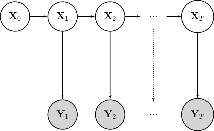
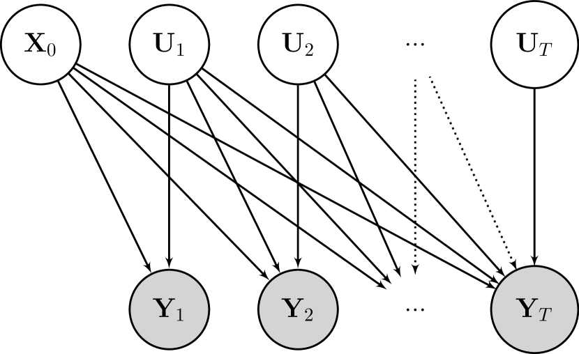
Figure 1: Graphical models of (a) the conventional state-space model, and (b) the disturbance state-space model. The $\mathbf{U}_{1:T}$ represent independent noise variables; conceptually, the disturbance state-space model simply reformulates the conventional model over these noise variables, the initial state, and the observations. Parameters, $\boldsymbol{\Theta}$, have been removed for clarity, but note that $\mathbf{U}_{1:T}\perp\!\!\!\perp\boldsymbol{\Theta}$, while all other variables depend on them.

For $T$ time points, a sequence of observations $\mathbf{y}_{1},\ldots,\mathbf{y}_{T}$ of random variables $\mathbf{Y}_{1},\ldots,\mathbf{Y}_{T}\in\mathbb{R}^{N_{y}}$ is assumed given, indicative of a latent initial condition $\mathbf{X}_{0}\in\mathbb{R}^{N_{x}}$ and latent states $\mathbf{X}_{1},\ldots,\mathbf{X}_{T}\in\mathbb{R}^{N_{x}}$. The model is parameterised by static $\boldsymbol{\Theta}\in\mathbb{R}^{N_{\theta}}$. The state transition is Markovian, and observations are conditionally independent given the states. This is the conventional state-space model, which takes the form

$$p(\mathbf{y}_{1:T},\mathbf{x}_{0:T},\boldsymbol{\theta})=\left[\prod_{t=1}^{T}p(\mathbf{y}_{t}|\mathbf{x}_{t},\boldsymbol{\theta})\right]\left[\prod_{t=1}^{T}p(\mathbf{x}_{t}|\mathbf{x}_{t-1},\boldsymbol{\theta})\right]p(\mathbf{x}_{0}|\boldsymbol{\theta})p(\boldsymbol{\theta}),$$ (1)

with the equivalent graphical model shown in Figure 1(a).

The transition density, $p(\mathbf{x}_{t}|\mathbf{x}_{t-1},\boldsymbol{\theta})$, may not have a closed form, or if it does, it may be too expensive to compute. This has been noted for diffusion processes [2, 9], and in fields such as biochemistry [11, 12], Functional Magnetic Resonance Imaging (fMRI) [26], and marine biogeochemistry [28]. In such cases it may be worth reformulating the model over its latent noise variables rather than its latent state variables. This can be done by explicitly introducing noise variables, $\mathbf{U}_{1:T}\in\mathbb{R}^{N_{u}}$, in place of $\mathbf{X}_{1:T}$. These may reflect, for example, independent Gaussian noise, or, in the most reduced form, the emissions of a pseudorandom number generator. The model can then be written:

$$p(\mathbf{y}_{1:T},\mathbf{u}_{1:T},\mathbf{x}_{0},\boldsymbol{\theta})=\left[\prod_{t=1}^{T}p(\mathbf{y}_{t}|\mathbf{u}_{1:t},\mathbf{x}_{0},\boldsymbol{\theta})\right]\left[\prod_{t=1}^{T}p(\mathbf{u}_{t})\right]p(\mathbf{x}_{0}|\boldsymbol{\theta})p(\boldsymbol{\theta}).$$ (2)

The equivalent graphical model is shown in Figure 1(b). We call this the disturbance state-space model. The conventional state-space model is recovered from it by introducing a deterministic function $f_{\theta}(\mathbf{u}_{t},\mathbf{x}_{t-1})\rightarrow\mathbf{x}_{t}$, permitting the recursive recovery of a state trajectory $\mathbf{x}_{1:t}$ from any sample $\{\mathbf{u}_{1:t},\mathbf{x}_{0}\}$.

In the disturbance state-space model the target becomes the posterior distribution over the random variables $\{\mathbf{U}_{1:T},\mathbf{X}_{0},\boldsymbol{\Theta}\}$, rather than the typical set $\{\mathbf{X}_{0:T},\boldsymbol{\Theta}\}$, and the tractable noise density, $p(\mathbf{u}_{t})$, emerges in place of the intractable transition density, $p(\mathbf{x}_{t}|\mathbf{x}_{t-1},\boldsymbol{\theta})$. The noise density is typically prescribed as having some simple parametric form, often Gaussian, with the $\mathbf{U}_{1:T}$ independent of each other and of other variables. This facilitates the design of proposal distributions when sampling, such as within an auxiliary particle filter, in cases where this is not possible under the conventional state-space model representation.

If $f_{\theta}(\cdot)$ is one-to-one, a change of variables for the transition density might be considered:

$$p(\mathbf{x}_{t}|\mathbf{x}_{t-1},\boldsymbol{\theta}) = p\left(f_{\theta}^{-1}\left(\mathbf{x}_{t}\right)|\mathbf{x}_{t-1},\boldsymbol{\theta}\right)\left|\frac{df_{\theta}^{-1}(\mathbf{x}_{t})}{d\mathbf{x}_{t}}\right|$$ (3)

$$= p(\mathbf{u}_{t})\left|\frac{df_{\theta}^{-1}(\mathbf{x}_{t})}{d\mathbf{x}_{t}}\right|.$$ (4)

When sampling from, say, $p(\mathbf{x}_{t}|\mathbf{x}_{t-1},\boldsymbol{\theta},\mathbf{y}_{1:t})$, one could likewise introduce an importance proposal $q(\mathbf{x}_{t}|\mathbf{x}_{t-1},\boldsymbol{\theta})=q(\mathbf{u}_{t})|df_{\theta}^{-1}(\mathbf{x}_{t})/d\mathbf{x}_{t}|$. In computing the importance weight, the Jacobian terms would cancel in the ratio, leaving $p(\mathbf{u}_{t})/q(\mathbf{u}_{t})$. Because this must formally assume that $f_{\theta}(\cdot)$ is one-to-one in order that the inverse $f^{-1}_{\theta}(\cdot)$ exists, however, we prefer the more-general approach of using the disturbance state-space model from the outset.

Reformulating to noise variables differs from the separation of tractable and intractable components in the Rao-Blackwellisation of state-space models [6], where it is typical to admit dependence of the tractable (linear) component on the intractable (nonlinear) component, but not vice-versa; in the disturbance state-space model, the intractable (nonlinear) component depends on the tractable (noise) component.

Roberts and Stramer [34] consider a similar idea to reparameterise a partially observed diffusion process for the purposes of Gibbs sampling. The advantage of doing so is that the conditional update of $\boldsymbol{\Theta}|\mathbf{u}_{1:T},\mathbf{x}_{0},\mathbf{y}_{1:T}$ is less constrained than that of $\boldsymbol{\Theta}|\mathbf{x}_{0:T},\mathbf{y}_{1:T}$, improving the mixing of the sampler. In this work, however, a Metropolis-Hastings rather than Gibbs update of $\boldsymbol{\Theta}$ is used, and no such advantage is conveyed. We pick up on this point in the discussion (§5).

There are alternative approaches to treat the absence of a closed-form transition density. One option is linearisation, such as an Euler-Maruyama [11, 9, 12] or local linearisation [27] of diffusion processes. This is not always workable, however, owing to some processes being unstable when discretised with low-order schemes. Higher-order or implicit discretisations are required in such cases, yielding complicated closed-form expressions, if they can be derived at all. A second option, supporting higher-order and implicit discretisations, is to simply choose a proposal distribution that cancels appearances of the transition density in weight evaluations [26]. The change-of-variables formulation above might be seen as an extension of this, cancelling just the intractable Jacobian term rather than the whole transition density. A third option is to unbiasedly estimate the transition density, if possible, as in the random-weight particle filter [9].

The use of the disturbance state-space model in a particle filtering context is given in §2 along with a suite of proposal configurations based on the unscented Kalman filter (UKF). We then turn to parameter estimation with the particle marginal Metropolis-Hastings (PMMH) sampler in §3, and introduce the criterion of conditional acceptance rate (CAR) to compare the performance of the various configurations. Two case studies in marine biogeochemistry are given in §4 with extensive empirical results. Concluding discussion appears in §5 and §6.

2 The auxiliary particle filter for the disturbance state-space model

For given $\{\mathbf{x}_{0},\boldsymbol{\theta}\}$, consider the joint filter density of the conventional state-space model:

$$p(\mathbf{x}_{t-1:t}|\mathbf{x}_{0},\boldsymbol{\theta},\mathbf{y}_{1:t})\propto p(\mathbf{y}_{t}|\mathbf{x}_{t},\boldsymbol{\theta})p(\mathbf{x}_{t}|\mathbf{x}_{t-1},\boldsymbol{\theta})p(\mathbf{x}_{t-1}|\mathbf{x}_{0},\boldsymbol{\theta},\mathbf{y}_{1:t-1}).$$ (5)

The analogue in the disturbance state-space model is

$$p(\mathbf{u}_{t},\mathbf{x}_{t-1}|\mathbf{x}_{0},\boldsymbol{\theta},\mathbf{y}_{1:t})\\ \propto p(\mathbf{y}_{t}|\mathbf{u}_{t},\mathbf{x}_{t-1},\boldsymbol{\theta})p(\mathbf{u}_{t})p(\mathbf{x}_{t-1}|\mathbf{x}_{0},\boldsymbol{\theta},\mathbf{y}_{1:t-1}).$$ (6)

Note that the complete noise history, $\mathbf{u}_{1:t}$, does not need to appear, as it is sufficient to recursively update and store $\mathbf{x}_{t}=f_{\theta}(\mathbf{u}_{t},\mathbf{x}_{t-1})$ as the filter progresses, with $\mathbf{x}_{0}$ establishing the base case of the recursion.

The auxiliary particle filter (APF) [29] is readily modified to sample from this. At time $t-1$, the APF maintains a set of $M$ particles $\mathbf{x}^{1:M}_{t-1}$ with associated weights $w^{1:M}_{t-1}$, normalised where required as $\tilde{w}^{m}_{t-1}=w^{m}_{t-1}/\sum_{i=1}^{M}w^{i}_{t-1}$. To advance to time $t$, an auxiliary lookahead propagation and weighting procedure [22] is used to produce stage-one weights $\omega_{t}^{1:M}$, again normalised where required as $\tilde{\omega}^{m}_{t}=\omega^{m}_{t}/\sum_{i=1}^{M}\omega^{i}_{t}$. For each particle $m$, an ancestor index $a^{m}_{t}$ is drawn from the categorical distribution $\mathcal{C}(\omega_{t}^{1:M})$, commonly called resampling (see e.g. Gordon et al. [13] or Kitagawa [20]). For the disturbance state-space model, the ancestor $\mathbf{x}^{a^{m}_{t}}_{t-1}$ is then extended by sampling $\mathbf{u}^{m}_{t}\sim q^{m}_{t}(\mathbf{u}^{m}_{t})$, where $q^{m}_{t}(\cdot)$ is some importance proposal for the $m$th particle, and setting $\mathbf{x}^{m}_{t}=f_{\theta}(\mathbf{u}^{m}_{t},\mathbf{x}^{m}_{t-1})$. The particle’s weight is then updated with

$$w^{m}_{t}=\frac{p(\mathbf{y}_{t}|\mathbf{x}^{m}_{t},\boldsymbol{\theta})p(\mathbf{u}^{m}_{t})}{q^{m}_{t}(\mathbf{u}^{m}_{t})}\cdot\frac{\tilde{w}^{a^{m}_{t}}_{t-1}}{\tilde{\omega}^{a^{m}_{t}}_{t}}.$$ (7)

This is called the stage-two weight. Code 1 gives this generic APF algorithm for the disturbance state-space model.

• $\textnormal{APF}(\mathbf{x}_{0},\boldsymbol{\theta})$
     1Initialise with $\mathbf{x}^{m}_{0}=\mathbf{x}_{0}$ and $\tilde{w}^{m}_{0}=1/M$ for $m=1,\ldots,M$. 2for $t=1,\ldots,T$ 3 for each $m\in\{1,\ldots,M\}$ 4 Compute stage-one weight $\omega^{m}_{t}$ 5 for each $m\in\{1,\ldots,M\}$ 6 $a^{m}_{t}\sim\mathcal{C}(\omega^{1:M}_{t})$ // resample 7 $\mathbf{u}^{m}_{t}\sim q^{m}_{t}(\mathbf{u}^{m}_{t})$ // propose 8 $\mathbf{x}^{m}_{t}\leftarrow f_{\theta}(\mathbf{u}^{m}_{t},\mathbf{x}^{a^{m}_{t}}_{t-1})$ // propagate 9 $w^{m}_{t}\leftarrow\frac{p(\mathbf{y}_{t}|\mathbf{x}^{m}_{t},\boldsymbol{\theta})p(\mathbf{u}^{m}_{t})}{q^{m}_{t}(\mathbf{u}^{m}_{t})}\cdot\frac{\tilde{w}^{a^{m}_{t}}_{t-1}}{\tilde{\omega}^{a^{m}_{t}}_{t}}$ // weight, stage two

Code 1: Generic auxiliary particle filter over a disturbance state-space model.

For the conventional state-space model, the locally optimal, or fully adapted proposal, is $q^{m}_{t}(\mathbf{x}^{m}_{t})\equiv p(\mathbf{x}^{m}_{t}|\mathbf{x}^{a^{m}_{t}}_{t-1},\boldsymbol{\theta},\mathbf{y}_{t})$ [29]. For the disturbance state-space model, its analogue is $q^{m}_{t}(\mathbf{u}^{m}_{t})\equiv p(\mathbf{u}^{m}_{t}|\mathbf{x}^{a^{m}_{t}}_{t-1},\boldsymbol{\theta},\mathbf{y}_{t})$. These cannot be derived analytically for the models of interest in this work, however, and so attention is given to reasonable approximations instead. Three such approximations are considered. The first scheme is the ordinary bootstrap particle filter [13]. The second and third use the UKF in different ways, the third similar to the existing unscented particle filter [39] but adapted to the disturbance state-space model. Each proposal scheme is tested both with and without a lookahead component for computing non-trivial stage-one weights, giving six methods in total. All six methods are detailed in this section and summarised in Table 1.

Method	Stage-one weight, $\omega^{m}_{t}$	Proposal, $q^{m}_{t}$	Number of propagations
PF0	$w^{m}_{t-1}$	$p(\mathbf{u}_{t})$	$M$
PF1	$p(\mathbf{y}_{t}|\mathbf{x}_{t}=f_{\theta}(\mathbf{0},\mathbf{x}^{m}_{t-1}),\boldsymbol{\theta})w^{m}_{t-1}$	$p(\mathbf{u}_{t})$	$2M$
MUPF0	$w^{m}_{t-1}$	$\hat{p}(\mathbf{u}_{t}|\mathbf{x}_{0},\boldsymbol{\theta},\mathbf{y}_{1:t})$	$M+2(N_{u}+N_{x}+N_{y})+1$
MUPF1	$p(\mathbf{y}_{t}|\mathbf{x}_{t}=f_{\theta}(\hat{\boldsymbol{\mu}}_{t},\mathbf{x}^{m}_{t-1}),\boldsymbol{\theta})w^{m}_{t-1}$	$\hat{p}(\mathbf{u}_{t}|\mathbf{x}_{0},\boldsymbol{\theta},\mathbf{y}_{1:t})$	$2M+2(N_{u}+N_{x}+N_{y})+1$
CUPF0	$w^{m}_{t-1}$	$\hat{p}^{m}(\mathbf{u}^{m}_{t}|\mathbf{x}^{a^{m}_{t}}_{t-1},\boldsymbol{\theta},\mathbf{y}_{1:t})$	$2M(N_{u}+N_{y}+1)$
CUPF1	$\hat{p}^{m}(\mathbf{y}_{t}|\mathbf{x}^{m}_{t-1},\boldsymbol{\theta})w^{m}_{t-1}$	$\hat{p}^{m}(\mathbf{u}^{m}_{t}|\mathbf{x}^{a^{m}_{t}}_{t-1},\boldsymbol{\theta},\mathbf{y}_{1:t})$	$2M(N_{u}+N_{y}+1)$

Table 1: Summary of the auxiliary particle filter proposal mechanisms explored. See §2 for details.

2.1 Bootstrap particle filter

The simplest approach, that of the bootstrap filter [13], sets

$$q^{m}_{t}(\mathbf{u}^{m}_{t})\equiv q_{t}(\mathbf{u}_{t})\equiv p(\mathbf{u}_{t}),$$ (8)

and

$$\omega^{m}_{t}=w^{m}_{t-1}.$$ (9)

This is straightforward to apply, and indeed does not benefit from reformulating the model over noise variables. Both the proposal and weights cancel in (7), so that particles are simply weighted by the likelihood $p(\mathbf{y}_{t}|\mathbf{x}^{m}_{t},\boldsymbol{\theta})$. We denote this method PF0.

Lacking $p(\mathbf{y}_{t}|\mathbf{x}_{t-1},\boldsymbol{\theta})$, an analytical lookahead is not forthcoming. A deterministic single-point pilot lookahead, simulating with $\mathbf{u}_{t}=\mathbf{0}$, can offer improvement in some cases [22]. By modifying the stage-one weights to

$$\omega^{m}_{t}=p(\mathbf{y}_{t}|\mathbf{x}_{t}=f_{\theta}(\mathbf{0},\mathbf{x}^{m}_{t-1}),\boldsymbol{\theta})w^{m}_{t-1},$$ (10)

we obtain a similar method with a lookahead, and denote it PF1.

2.2 Marginal unscented particle filter

We next attempt to draw on analytical approximations to inform the proposal distribution. The particular focus is on the UKF, which, for modest state sizes, tends to outperform [41] other approximate nonlinear Kalman filtering approaches, such as the extended [36] and ensemble [7, 8] variants. The UKF approximates the time marginals $p(\mathbf{u}_{t}|\mathbf{x}_{0},\boldsymbol{\theta},\mathbf{y}_{1:t})$ using a Gaussian distribution. We denote the approximation $\hat{p}(\mathbf{u}_{t}|\mathbf{x}_{0},\boldsymbol{\theta},\mathbf{y}_{1:t})\equiv\mathcal{N}(\hat{\boldsymbol{\mu}}_{t},\hat{\Sigma}_{t})$. At each time, $2(N_{u}+N_{x}+N_{y})+1$ number of $\sigma$-points are crafted about the mean of the Gaussian distribution, propagated through the process model and specifically weighted to compute a Gaussian approximation to $p(\mathbf{u}_{t},\mathbf{y}_{t}|\mathbf{x}_{0},\boldsymbol{\theta},\mathbf{y}_{1:t-1})$. Conditioning this on the actual observed value $\mathbf{y}_{t}$ delivers the approximate time marginal $\hat{p}(\mathbf{u}_{t}|\mathbf{x}_{0},\boldsymbol{\theta},\mathbf{y}_{1:t})$. See Julier and Uhlmann [17] and Wan and van der Merwe [41] for details.

The first UKF-based approach adopted is to use the marginal UKF approximations $\hat{p}(\mathbf{u}_{t}|\mathbf{x}_{0},\boldsymbol{\theta},\mathbf{y}_{1:t})$ at each time as a common proposal for each particle:

$$q^{m}_{t}(\mathbf{u}^{m}_{t})\equiv q_{t}(\mathbf{u}_{t})\equiv\hat{p}(\mathbf{u}_{t}|\mathbf{x}_{0},\boldsymbol{\theta},\mathbf{y}_{1:t})\equiv\mathcal{N}(\hat{\boldsymbol{\mu}}_{t},\hat{\Sigma}_{t}).$$ (11)

We call this the marginal unscented particle filter (MUPF), described in Code 2. By combining with the stage-one weights (9) we have the MUPF0 method. With stage-one weights

$$\omega^{m}_{t}=p(\mathbf{y}_{t}|\mathbf{x}_{t}=f_{\theta}(\hat{\boldsymbol{\mu}}_{t},\mathbf{x}^{m}_{t-1}),\boldsymbol{\theta})w^{m}_{t-1}$$ (12)

we have the MUPF1 method. Intuitively, using $f_{\theta}(\hat{\boldsymbol{\mu}}_{t},\mathbf{x}^{m}_{t-1})$ here seems more appealing than the $f_{\theta}(\mathbf{0},\mathbf{x}^{m}_{t-1})$ that appears in (10).

Note that the same time marginal $\hat{p}(\mathbf{u}_{t}|\mathbf{x}_{0},\boldsymbol{\theta},\mathbf{y}_{1:t})$ is used for each particle, not the conditional for the $m$th particle, $\hat{p}^{m}(\mathbf{u}^{m}_{t}|\mathbf{x}^{a^{m}_{t}}_{t-1},\boldsymbol{\theta},\mathbf{y}_{1:t})$, which is the basis for the next scheme. While the conditional proposal is no doubt preferable conceptually, the marginal proposal may be justifiable for fast-mixing models, and additionally enables the computational advantage of running the UKF offline from the particle filter. The overhead of the method is slight, with only $2(N_{u}+N_{x}+N_{y})+1$ additional propagations for the whole filter. This linear scaling with the number of dimensions is likely small compared to $M$, the number of particles, which would typically scale exponentially with the same.

• $\textnormal{MUPF}(\mathbf{x}_{0},\boldsymbol{\theta})$
      1Initialise with $\mathbf{x}^{m}_{0}=\mathbf{x}_{0}$ and $\tilde{w}^{m}_{0}=1/M$ for $m=1,\ldots,M$. 2Run a UKF to produce filtering densities $\hat{p}(\mathbf{u}_{t}|\mathbf{x}_{0},\boldsymbol{\theta},\mathbf{y}_{1:t})\equiv\mathcal{N}(\hat{\boldsymbol{\mu}}_{t},\hat{\Sigma}_{t})$, for $t=1,\ldots,T$. 3for $t=1,\ldots,T$ 4 for each $m\in\{1,\ldots,M\}$ 5 if doing MUPF1 6 $\hat{\mathbf{x}}^{m}_{t}\leftarrow f_{\theta}(\hat{\boldsymbol{\mu}}_{t},\mathbf{x}^{m}_{t-1})$ // look-ahead 7 $\omega^{m}_{t}\leftarrow p(\mathbf{y}_{t}|\hat{\mathbf{x}}^{m}_{t},\boldsymbol{\theta})w^{m}_{t-1}$ // weight, stage one 8 else doing MUPF0 9 $\omega^{m}_{t}\leftarrow w^{m}_{t-1}$ // weight, stage one 10 for each $m\in\{1,\ldots,M\}$ 11 $a^{m}_{t}\sim\mathcal{C}(\omega^{1:M}_{t})$ // resample 12 $\mathbf{u}^{m}_{t}\sim\mathcal{N}(\hat{\boldsymbol{\mu}}_{t},\hat{\Sigma}_{t})$ // propose 13 $\mathbf{x}^{m}_{t}\leftarrow f_{\theta}(\mathbf{u}^{m}_{t},\mathbf{x}^{a^{m}_{t}}_{t-1})$ // propagate 14 $w^{m}_{t}\leftarrow\frac{p(\mathbf{y}_{t}|\mathbf{x}^{m}_{t},\boldsymbol{\theta})p(\mathbf{u}^{m}_{t})}{q^{m}_{t}(\mathbf{u}^{m}_{t})}\cdot\frac{\tilde{w}^{a^{m}_{t}}_{t-1}}{\tilde{\omega}^{a^{m}_{t}}_{t}}$ // weight, stage two

Code 2: Marginal unscented particle filter (MUPF).

2.3 Conditional unscented particle filter

Finally, by conditioning the lookahead for each particle on the state of that particle, we arrive at the conditional unscented particle filter (CUPF), detailed in Code 3. It is similar to the unscented particle filter [39] but modified for the disturbance state-space model. The proposal is:

$$q^{m}_{t}(\mathbf{u}^{m}_{t})\equiv\hat{p}^{m}(\mathbf{u}^{m}_{t}|\mathbf{x}^{a^{m}_{t}}_{t-1},\boldsymbol{\theta},\mathbf{y}_{1:t})\equiv\mathcal{N}(\hat{\boldsymbol{\mu}}^{m}_{t},\hat{\Sigma}^{m}_{t}).$$ (13)

A UKF is run for each particle at each time step to construct this proposal distribution. Each UKF requires $2(N_{u}+N_{y})+1$ number of $\sigma$-point propagations, in addition to the subsequent propagation of the particle itself. This means $2M(N_{u}+N_{y}+1)$ propagations for the whole filter. Combined with the stage-one weights (9) we have the CUPF0 method. The alternative: rather than a single-point pilot lookahead, substantial improvement might be had by using the likelihood, marginalised over $\mathbf{u}_{t}$, that is approximated by the UKF:

$$\omega^{m}_{t}=\hat{p}^{m}(\mathbf{y}_{t}|\mathbf{x}^{m}_{t-1},\boldsymbol{\theta})w^{m}_{t-1}.$$ (14)

Use of these weights gives the CUPF1 method, which requires very little additional computation over CUPF0.

• $\textnormal{CUPF}(\mathbf{x}_{0},\boldsymbol{\theta})$
      1Initialise with $\mathbf{x}^{m}_{0}=\mathbf{x}_{0}$ and $\tilde{w}^{m}_{0}=1/M$ 2for $t=1,\ldots,T$ 3 for each $m\in\{1,\ldots,M\}$ 4 Run a UKF to produce $\hat{p}^{m}(\mathbf{u}_{t}|\mathbf{x}^{m}_{t-1},\boldsymbol{\theta},\mathbf{y}_{1:t})\equiv\mathcal{N}(\hat{\boldsymbol{\mu}}^{m}_{t},\hat{\Sigma}^{m}_{t})$. 5 if doing CUPF1 6 $\omega^{m}_{t}\leftarrow\hat{p}^{m}(\mathbf{y}_{t}|\mathbf{x}^{m}_{t-1},\boldsymbol{\theta})w^{m}_{t-1}$ // weight, stage one 7 else doing CUPF0 8 $\omega^{m}_{t}\leftarrow w^{m}_{t-1}$ // weight, stage one 9 for each $m\in\{1,\ldots,M\}$ 10 $a^{m}_{t}\sim\mathcal{C}(\omega^{1:M}_{t})$ // resample 11 $\mathbf{u}^{m}_{t}\sim\mathcal{N}(\hat{\boldsymbol{\mu}}^{m}_{t},\hat{\Sigma}^{m}_{t})$ // propose 12 $\mathbf{x}^{m}_{t}\leftarrow f_{\theta}(\mathbf{u}^{m}_{t},\mathbf{x}^{a^{m}_{t}}_{t-1})$ // propagate 13 $w^{m}_{t}\leftarrow\frac{p(\mathbf{y}_{t}|\mathbf{x}^{m}_{t},\boldsymbol{\theta})p(\mathbf{u}^{m}_{t})}{q^{m}_{t}(\mathbf{u}^{m}_{t})}\cdot\frac{\tilde{w}^{a^{m}_{t}}_{t-1}}{\tilde{\omega}^{a^{m}_{t}}_{t}}$ // weight, stage two

Code 3: Conditional unscented particle filter (CUPF).

3 The particle marginal Metropolis-Hastings sampler for the disturbance state-space model

For joint state and parameter estimation we target the posterior density $p(\mathbf{u}_{1:T},\mathbf{x}_{0},\boldsymbol{\theta}|\mathbf{y}_{1:T})$. This can be factorised as either:

$$p_{1}(\mathbf{u}_{1:T},\mathbf{x}_{0}|\boldsymbol{\theta},\mathbf{y}_{1:T})p_{2}(\boldsymbol{\theta}|\mathbf{y}_{1:T})$$ (15)

or

$$p_{1}(\mathbf{u}_{1:T}|\mathbf{x}_{0},\boldsymbol{\theta},\mathbf{y}_{1:T})p_{2}(\mathbf{x}_{0},\boldsymbol{\theta}|\mathbf{y}_{1:T}).$$ (16)

In either case, the first factor, $p_{1}(\cdot)$, is targeted using an APF, described in §2. The second factor, $p_{2}(\cdot)$, is targeted in an outer loop around the particle filter using Metropolis-Hastings (MH) [24, 14]. The particle filter nested within MH defines the particle marginal Metropolis-Hastings (PMMH) sampler, from the family of particle Markov chain Monte Carlo (PMCMC) methods [1].

Factorisation (15) requires that a good importance proposal is available for the sampling of $\mathbf{X}_{0}$ in the particle filter. If a good proposal is not available, the sample weights will be degenerate. In such cases (16) is the more attractive set up. It replaces the importance sample of $\mathbf{X}_{0}$ with local MH moves, which are typically easier to design. The factorisation (16) is used below.

In the outer loop, a proposed move from $\{\mathbf{x}_{0},\boldsymbol{\theta}\}$ to $\{\mathbf{x}^{\prime}_{0},\boldsymbol{\theta}^{\prime}\}\sim\rho(\mathbf{x}^{\prime}_{0},\boldsymbol{\theta}^{\prime}|\mathbf{x}_{0},\boldsymbol{\theta})$ is accepted with probability

$$\min\left[1,\frac{p(\mathbf{y}_{1:T}|\mathbf{x}^{\prime}_{0},\boldsymbol{\theta}^{\prime})p(\mathbf{x}^{\prime}_{0},\boldsymbol{\theta}^{\prime})\rho(\mathbf{x}_{0},\boldsymbol{\theta}|\mathbf{x}^{\prime}_{0},\boldsymbol{\theta}^{\prime})}{p(\mathbf{y}_{1:T}|\mathbf{x}_{0},\boldsymbol{\theta})p(\mathbf{x}_{0},\boldsymbol{\theta})\rho(\mathbf{x}^{\prime}_{0},\boldsymbol{\theta}^{\prime}|\mathbf{x}_{0},\boldsymbol{\theta})}\right],$$ (17)

where $\rho(\cdot)$ is a proposal distribution over parameters, and the marginal likelihoods $p(\mathbf{y}_{1:T}|\mathbf{x}^{\prime}_{0},\boldsymbol{\theta}^{\prime})$ are estimated by an APF targeting $p_{1}(\cdot)$ in (16). The estimator is [5, 1]:

$$p(\mathbf{y}_{1:T}|\mathbf{x}_{0},\boldsymbol{\theta})\approx\prod_{t=1}^{T}\left[\frac{1}{M}\sum_{m=1}^{M}w^{m}_{t}\right]$$ (18)

This assumes that normalised stage-one weights are used in computing stage-two weights, as in the preceding introduction. A proof of unbiasedness is given in Del Moral [5].

More rigorously, $p_{1}(\cdot)$ is a marginal of a distribution over the extended space in which the particle filter operates, a space that includes variables associated with the resampling mechanism [c.f. Equation 22 of 1]:

$$\psi(\mathbf{u}_{1:T}^{1:M},a_{1:T}^{1:M}|\mathbf{x}_{0},\boldsymbol{\theta})=\prod_{t=1}^{T}\left[r(a_{t}^{1:M}|w_{t-1}^{1:M})\prod_{m=1}^{M}p(\mathbf{u}_{t}^{m})\right].$$ (19)

Recall that $a_{t}^{m}$ is the index of the particle at time $t-1$ which is the ancestor of particle $m$ at time $t$. The function $r(\cdot)$ gives the probability of these. For some time $s\leq T$, let $b_{s}^{m}$ denote the index of the particle at time $s$ which is the ancestor of particle $m$ at time $T$, obtained by recursively tracing the ancestor indices backward through time, starting at $b^{m}_{T}=m$, then $b^{m}_{T-1}=a^{m}_{T},b^{m}_{T-2}=a^{b^{m}_{T-1}}_{T-1}$, and so forth. For some specific $m\sim\mathcal{C}(w^{1:M}_{T})$, a sample of $p_{1}(\cdot)$ is then given by the marginal $\{\mathbf{u}_{1}^{b_{1}^{m}},\ldots,\mathbf{u}_{T}^{b_{T}^{m}}\}$ [1].

PMMH chains can be “sticky” if the likelihood estimates from (18) are highly variable. A chain moving into a particular state on the basis of an unusually large likelihood estimate tends to remain there for a prolonged period before accepting a new proposal. The source of variability is both sampling and resampling error in the particle filter [30, 21]. The methods proposed in this work target a reduction of the former for any fixed number of particles. Furthermore, the likelihood estimates are heteroskedastic with respect to the parameters. For fixed $M$, the stickiness of a PMMH chain varies across the space of parameters, and from some regions a chain may not move to the vicinity of the posterior distribution in reasonable time. The problem is particularly acute when the process model informs the APF’s importance proposals, as in all of the strategies presented in §2. The effectiveness of the importance proposals is then a function of the likelihood of, and behaviours induced by, the current setting of the process model parameters. For example, small process noise variance parameters will produce narrow proposal distributions that may amplify weight variance, and so the variability of likelihood estimates. The mixing properties of the model may also be affected by gradient- and decay-related parameters.

3.1 Assessing the mixing of PMMH

To empirically explore the stickiness of PMMH chains under different particle filtering strategies, consider each point $(\mathbf{x}_{0},\boldsymbol{\theta})$ of a grid or set of points, and run some particle filtering method to be assessed $L$ times on each of those points. Each run $i$ can be interpreted as a sample from $\psi(\mathbf{u}_{1:T}^{1:M},a_{1:T}^{1:M}|\mathbf{x}_{0},\boldsymbol{\theta})$ in (19), and a marginal log-likelihood estimate $\hat{l}^{i}$ obtained (by using (18) and taking the logarithm). This gives $L$ log-likelihood estimates $\hat{l}^{1},\ldots,\hat{l}^{L}$.

At this point it is possible to compute a Monte Carlo estimate of the log-likelihood:

$$\mathbb{E}(l)\approx\bar{l}=\frac{1}{L}\sum_{i=1}^{L}\hat{l}^{i}.$$ (20)

and its standard deviation:

$$\sqrt{\mathbb{E}\left((l-\bar{l})^{2}\right)}\approx\sqrt{\frac{1}{L}\sum_{i=1}^{L}(\hat{l}^{i}-\bar{l})^{2}}.$$ (21)

This approach is taken in Pitt et al. [31] for a single central point of the posterior distribution. The idea is readily extended across a grid or set of values. Figure 2(a & b) do so, using the PZ model considered in §4.1. The model has two parameters, $\mu$ and $\sigma$. Estimates are made at each point of a 32 by 32 grid across the support of the uniform prior distribution over parameters. The surface is then interpolated using a Gaussian process fit by maximum likelihood, with a constant mean function, isotropic squared exponential covariance function and Gaussian likelihood [33, 32]. Pitt et al. [31] provides guidance to set the number of particles according to standard deviation estimates such as these.

We propose an alternative to standard deviation, which we call the conditional acceptance rate (CAR). The intuition is to approximate, at all points $(\mathbf{x}_{0},\boldsymbol{\theta})$ of a grid or set, the acceptance rate of a PMMH chain that starts at that point and remains there indefinitely by using a Dirac $\delta$-function proposal centred at that point. This can be seen as the limit of the acceptance rate when shrinking the proposal distribution. For conventional MH with an exact likelihood this will always be one, but for methods using a likelihood estimator, such as PMMH, this will be less than that owing to variance in the estimator. The CAR is always a number on $(0,1]$. While related to the standard deviation, the CAR is more directly interpretable as to the impact of variability in the likelihood estimator on the acceptance rate of a chain, and accommodates asymmetry in that variability. We prefer it for these reasons.

Consider a MH chain targeting $\psi(\mathbf{u}_{1:T}^{1:M},a_{1:T}^{1:M}|\mathbf{x}_{0},\boldsymbol{\theta})$, with independent proposal also $\psi(\mathbf{u}_{1:T}^{1:M},a_{1:T}^{1:M}|\mathbf{x}_{0},\boldsymbol{\theta})$, but restricted to the $L$ discrete states already drawn from it. The transition probability matrix $\mathbf{T}\in\mathbb{M}^{L\times L}$ of the chain is:

$$T_{ij}=\begin{cases}\frac{1}{L}\min\left[\exp(\hat{l}^{j}-\hat{l}^{i}),1\right]&\quad\text{if $i\neq j$}\\ 1-\sum_{\begin{subarray}{c}k=1\\ k\neq i\end{subarray}}^{L}T_{ik}&\quad\text{if $i=j$}.\end{cases}$$ (22)

$T_{ij}$ gives the probability of moving to the $j$th state, of log-likelihood $\hat{l}^{j}$, from the $i$th state, of log-likelihood $\hat{l}^{i}$. From state $i$, the probability of an acceptance occurring in the next step, marginalised over all possible proposals, is

$$\beta^{i}=1-T_{ii}+1/L.$$ (23)

The $1/L$ bias is incurred by using only a finite number of likelihood estimates.

From some arbitrary state, the Markov model defined by $\mathbf{T}$ may be run to equilibrium, where the probability of being in state $i$ is simply the normalised term

$$p^{i}=\frac{\exp\hat{l}^{i}}{\sum_{j=1}^{L}\exp\hat{l}^{j}}.$$ (24)

The long-term acceptance rate, which we refer to as the conditional acceptance rate at a given point, is then

$$CAR(\mathbf{x}_{0},\boldsymbol{\theta})=\sum_{i=1}^{L}p^{i}\beta^{i}.$$ (25)

Note that if all log-likelihood estimates are the same at a point, then $CAR(\mathbf{x}_{0},\boldsymbol{\theta})=1$. This is most easily seen through (25), as in this case $\beta^{i}=1$ for all $i=1,\ldots,L$, and the remaining sum over $p^{i}$ is necessarily 1. Given that a finite number of log-likelihood estimates are used, in the worst case $CAR(\mathbf{x}_{0},\boldsymbol{\theta})$ is still greater than $1/L$.

Figure 2(c) depicts the CAR surface computed across the same grid and same log-likelihood estimates as preceding plots in the same figure. This gives a clear picture that mixing is best in the high-likelihood region, declining with anisotropy away from that region.

In practice, the computation of CAR is simplified by following the procedure in Appendix A.

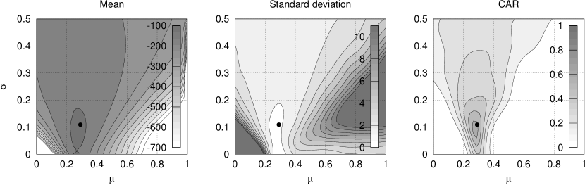
Figure 2: Surfaces of (a) the mean of log-likelihood estimates, (b) the standard deviation of log-likelihood estimates, and (c) the CAR, for a bootstrap particle filter on the PZ case study of §4.1. The CAR surface gives a good idea of how variability in the likelihood estimator impacts the acceptance rate of a PMMH sampler according to its current state.

4 Case studies in marine biogeochemistry

The proposed methods are assessed empirically on two models in the domain of marine biogeochemistry. All methods are assessed in each of two configurations, as in Table 2. The first is particle-matched, where the number of particles, $M$, is the same for all methods. The second is compute-matched, where $M$ is adjusted for all methods so as to roughly equate execution times. The latter is achieved by matching the total number of propagations, where these include lookahead pilots and UKF $\sigma$-points. We justify this by noting that for ordinary differential equation models such as those considered here, propagation typically dominates execution time (80-90% in these cases). By controlling the number of propagations, we roughly equate execution times in a fashion that is independent of any particular implementation in code.

Simulated data is used, generated from the case study models themselves. This has a number of advantages over real observational data: execution time can be managed to facilitate the many runs required for some diagnostics, the model is perfect in the generative sense, capturing all, and only, those processes influencing observations, and a known ground truth for all latent variables is available for validation of the methods. The second model is representative of real-world usage, however, and is fit to observational data using simpler PMMH methods in Parslow et al. [28].

		Particle-matched					Compute-matched
Case	Method	$M$	Acceptance		ESS		$M$	Acceptance		ESS
PZ	PF0	64	.182	(.003)	1444	(129)	384	.245	(.002)	2021	(196)
	PF1	64	.189	(.003)	1529	(141)	192	.233	(.002)	1926	(184)
	MUPF0	64	.208	(.003)	1707	(156)	376	.251	(.002)	2080	(200)
	MUPF1	64	.213	(.003)	1757	(162)	184	.243	(.002)	2008	(196)
	CUPF0	64	.209	(.003)	1709	(155)	64	.209	(.003)	1709	(155)
	CUPF1	64	.214	(.003)	1752	(159)	64	.214	(.003)	1752	(159)
NPZD	PF0	64	.142	(.003)	115	(8)	1536	.276	(.002)	163	(16)
	PF1	64	.139	(.006)	110	(9)	768	.254	(.003)	155	(14)
	MUPF0	64	.165	(.003)	123	(8)	1504	.278	(.002)	162	(16)
	MUPF1	64	.167	(.007)	121	(10)	736	.263	(.003)	157	(15)
	CUPF0	64	.169	(.003)	125	(10)	64	.169	(.003)	125	(10)
	CUPF1	64	.177	(.005)	125	(9)	64	.177	(.005)	125	(9)

Table 2: Configuration of methods for case studies, with mean (and standard deviation) of resulting acceptance rates and effective sample sizes across 256 chains. Chains for the PZ case study are run for 50000 steps, and those for the NPZD case study for 75000 steps. In computing ESS, autocorrelations are truncated at a lag of 100 with the first 10000 steps removed for the PZ case study, and truncated at a lag of 400 with the first 25000 steps removed for the NPZD case study. In the particle-matched configurations, improvements in acceptance rates and ESS are clear for the UKF-based proposal strategies (MUPF and CUPF). In compute-matched configurations there is no clear improvement on these metrics over the bootstrap methods (PF).

4.1 PZ model

The first model considered is a variant of the Lotka-Volterra differential system [23, 40], specifically over the predator-prey relationship of zooplankton and phytoplankton in a marine environment. Previously treated with a PMMH-style sampler [16], the intent here is to plumb deeper into the behaviour of the algorithm, the presence of just two parameters providing an ideal opportunity to visualise dependence of CAR on $\boldsymbol{\Theta}$. This PZ (phytoplankton and zooplankton) model modifies the classic Lotka-Volterra with the addition of a quadratic mortality term for zooplankton and a stochastic growth term for phytoplankton. The stochasticity admits varying growth rates in phytoplankton without explicitly modelling contributory factors such as light and temperature, and thus exemplifies how such uncertainties can be treated by the introduction of stochasticity into an otherwise deterministic model [16, 28].

The state of the model is given by $\mathbf{X}=\{P,Z,\alpha\}$, with $P$ and $Z$ denoting concentrations of phytoplankton and zooplankton, respectively, and $\alpha$ the stochastic growth rate of phytoplankton. These interact via:

$$\frac{dP}{dt} = \alpha_{t}P-cPZ$$ (26)

$$\frac{dZ}{dt} = ecPZ-m_{l}Z-m_{q}Z^{2}.$$ (27)

Here, $t$ is time in days, with prescribed constants $c=.25$, $e=.3$, $m_{l}=.1$ and $m_{q}=.1$. While $P$ and $Z$ are modelled in continuous time, the stochastic growth term, $\alpha_{t}$, is modelled in discrete time, updated daily using $\alpha_{t}\sim\mathcal{N}(\mu,\sigma)$. Parameters to be estimated are $\boldsymbol{\Theta}=\{\mu,\sigma\}$. Uniform prior distributions are assigned to the parameters, $\mu\sim\mathcal{U}(0,1)$ and $\sigma\sim\mathcal{U}(0,.5)$. Log-normal distributions are placed over the initial conditions, $\ln P\sim\mathcal{N}(\ln 2,.2)$ and $\ln Z\sim\mathcal{N}(\ln 2,.1)$. Phytoplankton ($P$) is observed with log-normal noise:

$$\ln Y_{P}\sim\mathcal{N}(\ln P,.2).$$ (28)

The differential equations must be numerically integrated forward in time. While an Euler discretisation would yield a closed-form transition density, the system is not numerically stable with such a low-order scheme. A fourth-order scheme, precisely the low-storage Runge-Kutta method RK4(3)5[2R+]C [4, 19], with adaptive time step, is used [25]. This does not readily yield a closed-form transition density, motivating the approach. Simulated data is used by integrating forward a single trajectory for 100 days, taking $P$ daily and adding observation noise.

The target is factorised as in (15), so that initial conditions are importance sampled within the particle filter. A systematic resampler [20] is used to minimise the contribution of the resampler to the variance of the likelihood estimator [30, 21]. To construct sensible starting and proposal distributions for the MH chain through $\boldsymbol{\Theta}$, a joint UKF (i.e. the state is augmented to include $\boldsymbol{\Theta}$) is first applied. The final filtering distribution, $\hat{p}(\boldsymbol{\theta}_{T}|\mathbf{y}_{1:T})\equiv\mathcal{N}(\hat{\boldsymbol{\mu}}_{T},\hat{\Sigma}_{T})$, is used as the starting distribution for the MH chain, and its covariance, $\hat{\Sigma}_{T}$, scaled by .18, for a random-walk Gaussian proposal. The scaling factor is chosen using pilot runs with the PF0 method. Starting at the rule-of-thumb $2.4^{2}/N_{\theta}=2.88$ [10] (recall $\Theta\in\mathbb{R}^{N_{\theta}}$), it is halved (four times) until a mixing rate close to the rule-of-thumb 23% [10] is achieved in the first 500 steps of the chain. Using this proposal, 256 PMMH chains of 50000 steps are then run for each method.

Performance is first assessed with established metrics. Trace plots for a single chain of the PF0 method with $M=64$ particles are given in Figure 3. These indicate good mixing. The other methods, not shown, produce traces that also indicate good mixing. Table 2 provides the mean and standard deviation of acceptance rates and effective sample sizes (ESS) across all chains for each method. The ESS is computed separately for each parameter of each chain [18]:

$$ESS=1+2\sum_{k=1}^{\infty}R(k,\theta),$$ (29)

where $R(k,\theta)$ is the lag-$k$ autocorrelation of the single parameter $\theta$. The first 10000 steps are removed as burn-in and the infinite sum truncated at $k=100$. The minimum ESS across all parameters of a chain is then taken as that chain’s overall ESS for reporting in Table 2. Finally, the multivariate $\hat{R}^{p}$ statistic of Brooks and Gelman [3] is computed across all chains to empirically assess the rate of convergence (Figure 4). All of these metrics establish that the chains are mixing well.

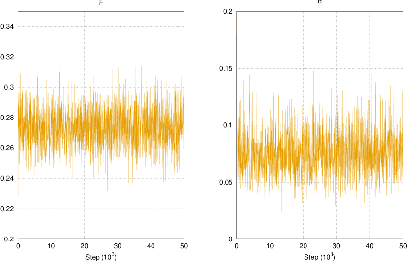
Figure 3: Indicative trace plots of a single PMMH chain over parameters of the PZ model, using the PF0 method with 64 particles. These indicate good mixing of the chain. Other methods use the same proposal and achieve higher acceptance rates (Table 2); their trace plots, while not shown, appear at least as good on inspection.

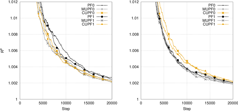
Figure 4: Convergence rates of Markov chains for the PZ case study, (a) particle-matched, and (b) compute-matched. Each line shows the evolution of the $\hat{R}^{p}$ statistic of Brooks and Gelman [3] for a particular method as the number of steps taken increases. The statistic is computed using 256 chains for each method. A more rapid approach to 1 indicates faster convergence. In the particle-matched configuration the UKF-based methods demonstrate faster convergence. In the compute-matched configuration the MUPF methods may give a slight improvement over the simpler PF methods.

The posterior distribution obtained over parameters is marked in Figures 6 and 7, using samples drawn across all chains for each method. For one chain, the state posterior is visualised in Figure 5, along with the ground truth trajectory and observations for comparison.

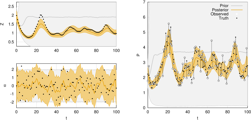
Figure 5: Time-marginal posteriors over state variables ($P$ and $Z$) and noise term ($\alpha$) for the PZ case study. Results are obtained by PMMH using the CUPF1 method. Other methods give comparable results, although not shown. The bold centre lines of the prior and posterior distributions denote their medians, and the shaded regions their 95% credibility intervals.

With results looking sensible so far, we proceed with a comparison using the CAR metric introduced in §3.1. For each method, the CAR is computed at 1024 points on a 32 by 32 regular grid across the uniform prior distribution, using 200 likelihood evaluations at each point. To produce contours of the surface, a Gaussian process is fit to the points by maximum likelihood, with a constant mean function, isotropic squared exponential covariance function and Gaussian likelihood [33, 32]. Results are presented for particle-matched configurations in Figure 6, and for compute-matched in Figure 7.

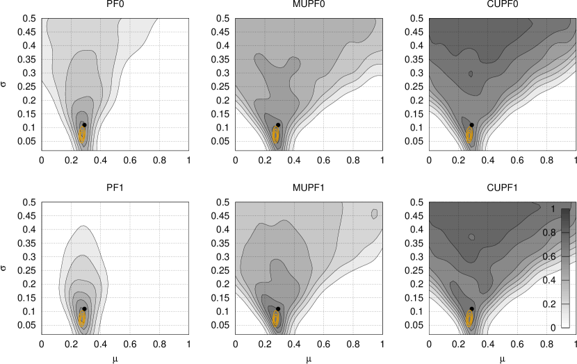
Figure 6: CAR surfaces for the PZ case study across the support of the uniform prior distribution over parameters. Each plot shows the results for a particular method in its particle-matched configuration. Darker shading denotes higher CAR (see key bottom right). The dots at approximately (0.3, 0.1) in each plot mark the ground truth parameters from which the data set is simulated. The bold contours nearby mark the posterior distribution obtained. A clear decline in CAR is evident as distance increases from the ground truth and posterior region. The CUPF methods appear more robust than others at high $\sigma$.

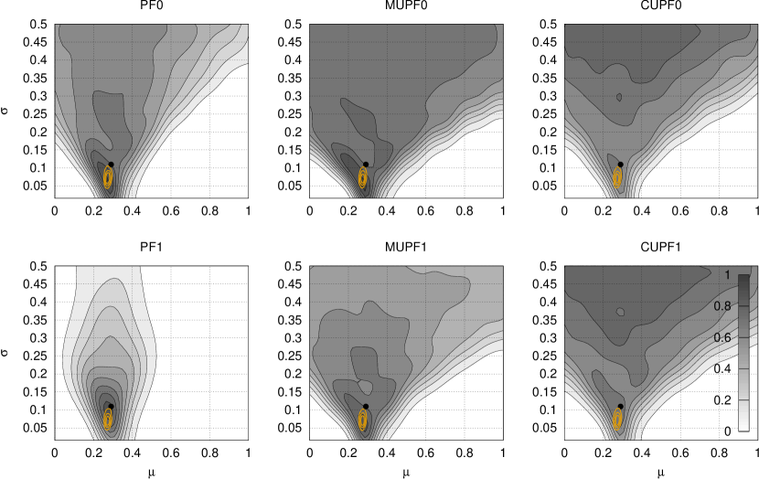
Figure 7: CAR surfaces for the PZ case study for compute-matched configurations. See Figure 6 caption for details.

4.2 NPZD model

The introduction of nutrients, $N$, and detritus, $D$, into the PZ model provides a more realistic system with which real observational data can begin to be assimilated: an NPZD model. These additional terms are accompanied by various environmental forcings and rate processes that produce a more challenging model, with nonlinear responses ranging from convergence, to periodicity, to chaos. The full details and motivation behind the model are given in Parslow et al. [28]. A brief description to elucidate some of the complexity is given here.

The NPZD model represents the interaction of nutrients ($N$), phytoplankton ($P$), zooplankton ($Z$) and detritus ($D$), quantified in the common currency of nitrogen, within the surface mixed layer of a body of water. The surface waters are modelled as a single box, subject to exogenous environmental forcings such as available light, temperature and changes in mixed layer depth.

4.2.1 Noise model

The model features nine noise terms, $\xi_{i}$ for $i=1,\ldots,9$, each coupled to a univariate autoregressive process $B_{i}$. Four of these are phytoplankton-related, given by

$$B_{i}(t+\Delta t)=B_{i}(t)\cdot(1-\Delta t/\tau_{P})+(\mu_{i}+PDF\cdot\sigma_{i}\xi_{i})\cdot\Delta t/\tau_{P},$$ (30)

where $\Delta t$ is a discrete time step (one day), $\mu_{i}$ a parameter to be estimated, $PDF$ a common diversity factor parameter to be estimated, $\sigma_{i}$ a prescribed scaling factor, and $\tau_{P}$ a common characteristic time scale, also prescribed. The remaining five autoregressive processes are zooplankton-related, modelled using the same form, with $ZDF$ and $\tau_{Z}$ replacing $PDF$ and $\tau_{P}$, respectively.

Each process represents a property of the phytoplankton (zooplankton) community, the species composition of which will change with time. Rather than model individual species, the phytoplankton (zooplankton) community is modelled collectively, with diversity factors $PDF$ and $ZDF$ scaling stochastic drivers used to model the changing influence of community composition.

The four phytoplankton processes are $\{g^{\text{max}},\lambda^{\text{max}},R_{N},a_{N}\}$, and the five zooplankton processes $\{I_{Z},Cl_{Z},E_{Z},r_{D},m_{Q}\}$. Each is accompanied by its matching noise term amongst $\{\xi_{g^{\text{max}}},$ $\xi_{\lambda^{\text{max}}},$ $\xi_{R_{N}},$ $\xi_{a_{N}},$ $\xi_{I_{Z}},$ $\xi_{Cl_{Z}},$ $\xi_{E_{Z}},$ $\xi_{r_{D}},$ $\xi_{m_{Q}}\}$, and mean parameter amongst $\{\mu_{g^{\text{max}}},$ $\mu_{\lambda^{\text{max}}},$ $\mu_{R_{N}},$ $\mu_{a_{N}},$ $\mu_{I_{Z}},$ $\mu_{Cl_{Z}},$ $\mu_{E_{Z}},$ $\mu_{r_{D}},$ $\mu_{m_{Q}}\}$.

4.2.2 Process model

The remaining state variables are $\{N,P,Z,D\}$ and parameters $\{K_{W},$ $a_{Ch},$ $S_{D},$ $f_{D}\}$. The equations governing interactions between the remaining state variables are:

$$\frac{dN}{dt} = -g\cdot P+(1-E_{Z})\cdot(1-f_{D})\cdot gr\cdot Z+r\cdot D+\frac{\kappa}{MLD}\cdot(BCN-N)$$ (31)

$$\frac{dP}{dt} = g\cdot P-gr\cdot Z+\frac{\kappa}{MLD}\cdot(BCP-P)$$ (32)

$$\frac{dZ}{dt} = E_{Z}\cdot gr\cdot Z-m\cdot Z$$ (33)

$$\frac{dD}{dt} = (1-E_{Z})\cdot f_{D}\cdot gr\cdot Z+m\cdot Z-r\cdot D-S_{D}\cdot\frac{D}{MLD}+\frac{\kappa}{MLD}\cdot(BCD-D).$$ (34)

Here, $g$ is the phytoplankton specific growth rate (per day, or d^-1), $gr$ is the zooplankton specific grazing rate (mg $P$ grazed per mg $Z$ d^-1), $m$ is the zooplankton specific mortality rate (d^-1), and $r$ is the specific breakdown rate of detritus (d^-1). A fraction, $E_{Z}$, of zooplankton ingestion is converted to zooplankton growth and, of the remainder, a fraction, $f_{D}$, allocated to detritus and the rest released as dissolved inorganic nutrient, $N$.

The rate processes $gr$, $m$ and $g$ are not only functions of the state, but also prescribed exogenous forcings and physiological constants. A multiplicative temperature correction $Tc$ is applied to all of these, for which a $Q_{10}$ formulation for dependence on temperature, $T$, is used:

$$Tc=Q_{10}^{(T-T_{\text{ref}})/10},$$ (35)

where $T_{\text{ref}}$ is a reference temperature, and $Q_{10}$ a prescribed constant.

The zooplankton grazing rate, $gr$, is dependent on the relative availability of phytoplankton, $A$:

$$gr=\frac{Tc\cdot I_{Z}\cdot A^{\upsilon}}{(1+A^{\upsilon})},$$ (36)

where $\upsilon$ is a given power, and

$$A=\frac{Cl_{Z}\cdot P}{I_{Z}}.$$ (37)

$I_{Z}$ is the maximum zooplankton ingestion rate (mg $P$ per mg $Z$ per day); $Cl_{Z}$ is the maximum clearance rate (volume in m³ swept clear per mg $Z$ per day). For $\upsilon=1$, (36) takes the form of a Type-2 functional response (standard rectangular hyperbola) [15], and for $\upsilon>1$ a Type-3 sigmoid functional response.

A quadratic formulation for zooplankton mortality is adopted after Steele [37] and Steele and Henderson [38]:

$$m=Tc\cdot m_{Q}\cdot Z,$$ (38)

where the quadratic mortality rate, $m_{Q}$, has units of d${}^{-1}(\text{mg}Z\text{m}^{-3})^{-1}$. The detrital remineralisation rate is dependent only on temperature:

$$r=Tc\cdot r_{D},$$ (39)

where $r_{D}$ prescribes the remineralisation rate at a reference temperature.

The phytoplankton specific growth rate, $g$, depends on temperature, $T$, available light or irradiance, $E$, and dissolved inorganic nutrient, $N$. It is expressed in terms of a maximum specific growth rate at the reference temperature, $g^{\text{max}}$ (d^-1), a light-limitation factor, $h_{E}$, and a nutrient-limitation factor, $h_{N}$:

$$g=Tc\cdot g^{\text{max}}\cdot h_{E}\cdot h_{N}/(h_{E}+h_{N}).$$ (40)

The light-limitation factor is given by

$$h_{E}=1-\exp(-\alpha\cdot\lambda^{\text{max}}\cdot E/g^{\text{max}}),$$ (41)

where $\alpha$ is the initial slope of the photosynthesis versus irradiance curve (mg $C$ mg $Chla^{-1}$ mol photon^-1 m²), and $\lambda^{\text{max}}$ is the maximum $Chla:C$ (chlorophyll-a to carbon) ratio (mg $Chla$ mg $C^{-1}$). Here, $\alpha$ is calculated as the product of the chlorophyll-specific absorption coefficient for phytoplankton, $a_{Ch}$ (m² mg $Chla^{-1}$), and the maximum quantum yield for photosynthesis, $Q$ (mg $C$ mol photons^-1). $E$ is the mean photosynthetic available radiation (PAR) in the mixed layer and is given by

$$E=E_{0}\cdot(1-\exp(-Kz))/Kz,$$ (42)

where $E_{0}$ is the mean daily photosynthetically available radiation (PAR) just below the air-sea interface, $Kz$ is given by

$$Kz=(K_{W}+a_{Ch}\cdot Chla)\cdot MLD.$$ (43)

and $K_{W}$ is attenuation due to the seawater and $a_{Ch}$.

The nutrient-limitation factor is given by

$$h_{N}=\frac{N}{(g^{\text{max}}\cdot Tc/a_{N})+N},$$ (44)

where $a_{N}$ is the maximum specific affinity for nitrogen uptake (d^-1 mg $N^{-1}$ m³).

The phytoplankton $N:C$ (nitrogen to carbon) ratio, $\chi$, predicted by the model is given by

$$\chi=\frac{\chi^{\text{min}}\cdot h_{E}+\chi^{\text{max}}\cdot h_{N}}{h_{E}+h_{N}},$$ (45)

where $\chi^{\text{min}}$ and $\chi^{\text{max}}$ are the prescribed minimum and maximum $N:C$ ratios (mg $N$ mg $C^{-1}$).

4.2.3 Boundary conditions

The simple single-box mixed layer model adopted here needs to allow for the effects of physical exchanges between the mixed layer and the underlying water mass. With the exception of $BCN$, all boundary conditions ($BCP,BCD,BCZ$) are set to zero for the experiments in this work. The variable $\kappa$ sets the strength of the mixing; in this study, we assume that the lower two metres of the mixed layer are replenished daily with water from below. $MLD$ and $BCN$ are in this case time-invariant, and set to 40 m and 200 mg N m³, respectively.

4.2.4 Observation model

The model predicts the phytoplankton $Chla:C$ ratio $\lambda$, and this can be combined with the $N:C$ ratio $\chi$ to convert phytoplankton biomass $P$ (mg $N$ m^-3) to a predicted $Chla$ concentration:

$$Chla=P\cdot(\lambda^{\text{max}}/\chi^{\text{max}})\cdot h_{N}\cdot Tc/(R_{N}\cdot h_{E}+h_{N}).$$ (46)

Both $N$ and $Chla$ are observed, each with log-normal noise of 40%, i.e. $\ln Y_{N}\sim\mathcal{N}(\ln N,.4)$, and $\ln Y_{Chla}\sim\mathcal{N}(\ln Chla,.4)$. Observations are thus written $\mathbf{Y}=\{Y_{N},Y_{Chla}\}$.

4.2.5 Experiments

The fourth order Runge-Kutta scheme RK4(3)5[2R+]C [19] is again used to numerically integrate the differential equations forward. Use of such a higher-order scheme is essential for this model, which is unstable under low-order schemes like Euler. A data set is generated by simulating the model with artificial forcing for 100 days, from which nutrient ($N$) and chlorophyll-a ($Chla$) observations are produced daily. A systematic resampler [20] is again used.

The target is factorised according to (16), so that both parameters and initial conditions are sampled by the MH chain. To construct sensible starting and proposal distributions, a joint UKF is first applied, in the same way as for the PZ model. Because starting and proposal distributions over both parameters and initial conditions are now required, we then apply a joint unscented Rauch-Tung-Striebel smoother (URTSS) [35] to the output of the UKF, giving a Gaussian approximation to the smoothing distribution $p(\mathbf{x}_{0},\boldsymbol{\theta}_{0}|\mathbf{y}_{1:T})$. This is taken as the starting distribution for the MH chain, and its covariance, scaled by .012, for a random-walk Gaussian proposal. Figure 8 shows a comparison of the covariance matrix obtained by URTSS to that eventually obtained by PMMH; the similarity makes clear the utility of the approach in constructing a sensible proposal distribution. Using this proposal, 256 PMMH chains of 75000 steps are then run for each method.

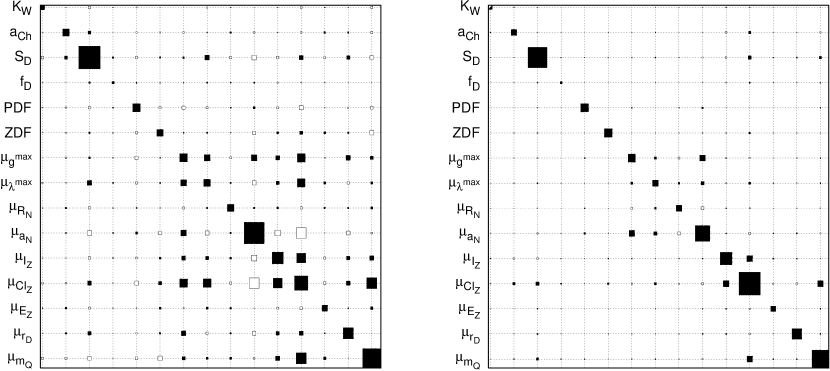
Figure 8: Covariance matrices over parameters of the NPZD model, as returned by (a) PMMH using CUPF1, and (b) URTSS. The area of each square is proportional to magnitude, with filled squares denoting positive, and empty squares negative, covariance. The covariance matrices for initial conditions and cross-covariance (neither shown) also show similarity, although there is little interesting off-diagonal structure. While approximate, the URTSS method is inexpensive, and still captures some significant off-diagonal elements that can be used to construct a good proposal distribution for PMMH.

Trace plots for a single chain of the PF0 method are given in Figure 9. Table 2 provides the mean and standard deviation of acceptance rates and ESS across all chains for each method. In computing ESS, the first 25000 samples from each chain are removed as burn-in, and the infinite sum truncated at a lag of $k=400$. The $\hat{R}^{p}$ statistic [3] is computed across multiple chains and shown in Figure 10. All of these metrics indicate reasonable mixing, albeit with effective sample size significantly lower than in the PZ case study. The univariate posterior marginal distributions of parameters and state are given in Figures 11 and 12.

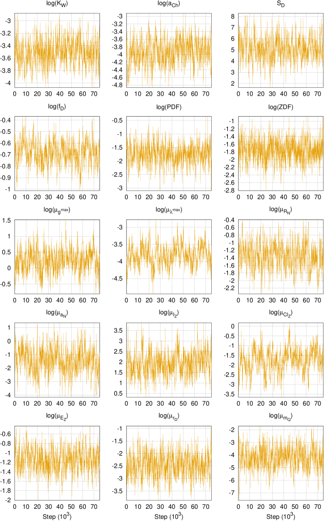
Figure 9: Indicative trace plots of a single PMMH chain over parameters of the NPZD model, using the PF0 method with 64 particles. These indicate reasonable mixing of the chain. Some autocorrelation is apparent, reducing ESS in Table 2.

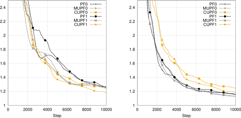
Figure 10: Convergence rates of Markov chains for the NPZD case study, (a) particle-matched, and (b) compute-matched. See Figure 4 caption for details. In particle-matched configurations the UKF-based methods offer a clear improvement, but in compute-matched configurations the simpler PF0 and PF1 methods are again competitive.

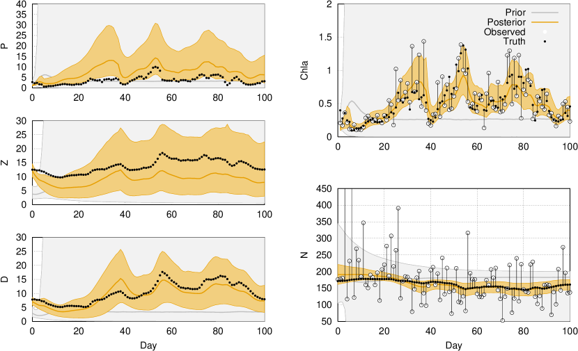
Figure 11: Time-marginal posterior distributions over state variables for the NPZD case study. Results are obtained by PMMH using the CUPF1 method. Other methods give comparable results, although not shown. The bold centre lines of the prior and posterior distributions denote their medians, and the shaded regions their 95% credibility intervals.

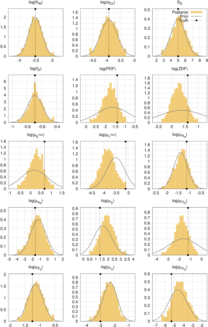
Figure 12: Prior and posterior distributions over parameters for the NPZD case study. Results are obtained by PMMH using the CUPF1 method.

CARs are computed at a set of 4096 points drawn randomly from the prior distribution. Because of the higher dimensionality of the NPZD model, plots such as Figures 6 and 7 produced for the PZ model are not feasible. Instead, pairwise copulas between parameters and the CAR, computed empirically, are shown in Figure 14, with the empirical cumulative distribution function of the same CARs shown in Figure 13.

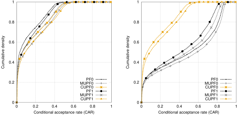
Figure 13: Empirical cumulative distribution functions of the CAR for each method on the NPZD case study, (a) particle-matched, and (b) compute-matched. For each method, the CAR is computed at the same sample points used to construct Figure 14. The empirical cumulative distribution function over all of these CARs is then evaluated. As higher CARs are preferred, a lower cumulative density on the $y$-axis is preferred for any given point on the $x$-axis. An advantage for the UKF-based methods is apparent in the particle-matched case, but this is only maintained for the MUPF0 method in the compute-matched case.

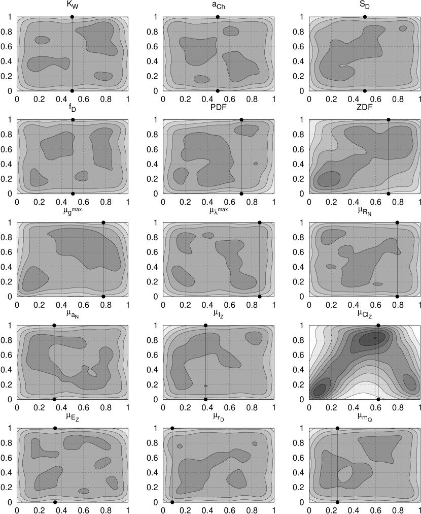
Figure 14: Estimated copula functions between parameters ($x$-axes) and CAR ($y$-axes) for the NPZD case study, using the CUPF1 method. Other methods give similar results. For parameters, the prior univariate cumulative density functions are used for transformation to uniform marginals. For the CAR, the empirical cumulative density function is used. The copula function is approximated using a kernel density estimate of bandwidth .075 over the 4096 points sampled from the prior distribution over parameters, with the CAR computed at each point using 200 likelihood evaluations. Edge effects are an artifact of the kernel density estimate. Most striking is the significant sensitivity of the CAR to the $\mu_{Cl_{Z}}$ parameter, explained in the text.

5 Discussion

When the number of particles is matched across methods, the MUPF and CUPF methods outperform the basic PF methods for both the PZ and NPZD cases: in acceptance rate and ESS (Table 2), convergence rates (Figures 4(a) and 10(a)) and CAR (Figures 6 and 13(a)). For the PZ model, the lookahead degrades performance for PF1 and MUPF1, but not for CUPF1. This is presumably because the single-point pilots used in the first two methods are not representative of the whole predictive distribution. For the NPZD model, the lookahead is beneficial. This is attributed to the NPZD model having longer memory than the faster-mixing PZ model, a scenario where lookaheads tend to be more useful.

In compute-matched configurations, the MUPF methods appear to retain some advantage in the PZ case study: in acceptance rate and ESS (Table 2), convergence rates (Figure 4(b)) and CAR (Figure 7). In the NPZD case study, overall acceptance rates and ESS are very similar to the simpler PF methods (Table 2), although there is some suggestion that at least the MUPF0 method retains an advantage in CAR across the space of parameters (Figure 13(b)). The CUPF methods appear to offer no overall advantage in compute-matched configurations, but an interesting subplot arises from the CUPF methods in the PZ case study: no other methods match the CARs achieved by them in low-likelihood regions, even after correction for compute time (Figures 6 and 7). This suggests that these methods may make a more robust choice for early steps in a PMMH chain if a good initialisation is unavailable, later displaced by one of the cheaper methods once in a region of higher likelihood.

The MUPF method performs significantly better on the PZ model than the NPZD model, and the PZ model is known to mix faster than the NPZD model. This is consistent with the expectation that the MUPF methods should work better for faster mixing models. An outstanding challenge is to design more generally applicable proposal schemes for the disturbance state-space model that are computationally competitive, and deliver more convincing outcomes for harder cases such as the NPZD model. This is left to future work. There is, however, evidence here that there exist proposals, enabled by the disturbance state-space model formulation, that can improve PMMH performance in some circumstances.

The CAR, introduced in this work, is one means of assessing the impact of variance in a particle filter’s likelihood estimator on the acceptance rate of a PMMH chain. Computing the CAR at multiple points in parameter space for both the PZ (Figures 6 and 7) and NPZD (Figure 13) cases is revealing. For the PZ model, a clear decline in CAR away from the region of high likelihood is apparent (Figures 2, 6 and 7), although larger values of the diffusion parameter $\sigma$ lend improvement. The NPZD case is more complex, with many parameters having no apparent correlation with CAR over the support of their prior distribution (Figure 14). Again, however, there is some indication that larger values of diffusion parameters (especially $ZDF$) improve CAR. There is a strong relationship with one parameter, $\mu_{Cl_{Z}}$, to which the model is known to be particularly sensitive.

The dependence of CAR on diffusion parameters is not surprising when the process model informs the APF proposal distribution: the broader distributions induced by larger values of diffusion parameters tend to make better importance proposals, up to a point. For the PZ model, given the uniform prior over parameters, the maximum a posteriori (MAP) estimate of the parameters is also the maximum likelihood estimate (MLE) of the parameters, assuming that the latter falls within the support of the prior. For the NPZD model, we might assume that the MLE is close to the ground truth. CAR appears highest at these MLEs, and declines with distance from them. We conjecture that this may be a general property, and stress the MLE, not the MAP: the prior distribution over parameters does not factor into the likelihood estimator of the particle filter, so the MAP should be relevant only insofar as it is influenced by the likelihood.

Given the variability of the CAR, there are two potential pitfalls to avoid when using a PMMH sampler: (i) initialisation in a region where CAR is low, and (ii) having a particularly informative prior distribution that biases the posterior into a region where CAR is low. Either case may result in too much stickiness for the PMMH chain to converge in reasonable time. These should be considered failure modes of the PMMH sampler in much the same way as strongly correlated variables can cause slow mixing in the Gibbs sampler, or multiple modes can cause quasiergodicity in any Markov chain Monte Carlo algorithm. The CAR is a useful diagnostic for such behaviour.

An alternative approach to PMMH is that of particle Gibbs [1]. In place of the Metropolis-Hastings update of $\boldsymbol{\Theta}$, this involves a Gibbs (or Metropolis-Hastings-within-Gibbs) update of $\boldsymbol{\Theta}|\mathbf{u}_{1:T},\mathbf{x}_{0},\mathbf{y}_{1:T}$. While not considered in this work, it is worth noting that the disturbance state-space model representation may produce better mixing than the conventional state-space model when sampled with particle Gibbs, because $\boldsymbol{\Theta}|\mathbf{u}_{1:T},\mathbf{x}_{0},\mathbf{y}_{1:T}$ is less constrained than $\boldsymbol{\Theta}|\mathbf{x}_{0:T},\mathbf{y}_{1:T}$. The justification is the same as that considered in Roberts and Stramer [34].

6 Conclusion

In the absence of a closed-form transition density, the disturbance state-space model seems a generally good approach to enabling cleverer proposal strategies in the APF. This work establishes some utility in doing so, particularly for fast-mixing models, by drawing on two specific case studies in marine biogeochemistry. In these cases the performance of PMMH chains is shown to improve in some situations by using UKF-based proposals, as judged by acceptance rate, ESS, convergence rate and CAR. These empirical results also elucidate some of the behaviours peculiar to the PMMH sampler, such as the heteroskedasticity of the likelihood estimator, and the implied need for a good initialisation. The development of robust, generally applicable and computationally competitive proposal strategies for the APF in this context remains outstanding work.

Appendix A Computing the conditional acceptance rate

A simple way to compute the CAR is to first compute the equilibrium probabilities using (24) and sort them into ascending order. Let $\mathbf{c}$ be the vector of inclusive prefix-sums over the sorted vector $\mathbf{p}$:

$$c^{i}=\sum_{j=1}^{i}p^{j}.$$ (47)

Now proceed as follows:

$$\beta^{i}=\frac{1}{L}\left[\frac{c^{i}}{p^{i}}+L-i\right].$$ (48)

Substituting into (25):

$$CAR(\mathbf{x}_{0},\boldsymbol{\theta}) = \frac{1}{L}\sum_{i=1}^{L}p^{i}\left[\frac{c^{i}}{p^{i}}+L-i\right]$$ (49)

$$= \frac{1}{L}\left[\sum_{i=1}^{L}c^{i}+\sum_{i=1}^{L}p^{i}(L-i)\right]$$ (50)

$$= \frac{1}{L}\left[\sum_{i=1}^{L}c^{i}+\sum_{i=1}^{L}(c^{i}-p^{i})\right]$$ (51)

$$= \frac{1}{L}\left[2\sum_{i=1}^{L}c^{i}-1\right].$$ (52)

References

- Andrieu et al. [2010] C. Andrieu, A. Doucet, and R. Holenstein. Particle Markov chain Monte Carlo methods. Journal of the Royal Statistical Society Series B, 72:269–302, 2010.
- Beskos et al. [2006] A. Beskos, O. Papaspiliopoulos, G. Roberts, and P. Fearnhead. Exact and efficient likelihood-based inference for discretely observed diffusion processes (with discussion). Journal of the Royal Statistical Society Series B, 68:333–382, 2006.
- Brooks and Gelman [1998] S. P. Brooks and A. Gelman. General methods for monitoring convergence of iterative simulations. Journal of Computational and Graphical Statistics, 7:434–455, 1998.
- Carpenter and Kennedy [1994] M. H. Carpenter and C. A. Kennedy. Fourth-order 2N-storage Runge-Kutta schemes. Technical Report Technical Memorandum 109112, National Aeronautics and Space Administration, June 1994.
- Del Moral [2004] P. Del Moral. Feynman-Kac Formulae: Genealogical and Interacting Particle Systems with Applications. Springer, 2004.
- Doucet et al. [2000] A. Doucet, N. de Freitas, K. Murphy, and S. Russel. Rao-Blackwellised particle filtering for dynamic Bayesian networks. In Proceedings of the 16th Conference on Uncertainty in Artificial Intelligence, pages 176–183, 2000.
- Evensen [1994] G. Evensen. Sequential data assimilation with a nonlinear quasi-geostrophic model using Monte-Carlo methods to forecast error statistics. Journal of Geophysical Research-Oceans, 99(C5):10143–10162, 1994. ISSN 0148-0227.
- Evensen [2009] G. Evensen. The ensemble Kalman filter for combined state and parameter estimation. IEEE Control Systems Magazine, 29:83–104, 2009.
- Fearnhead et al. [2008] P. Fearnhead, O. Papaspiliopoulos, and G. O. Roberts. Particle filters for partially observed diffusions. Journal of the Royal Statistical Society Series B, 70:755–777, 2008.
- Gelman et al. [1994] A. Gelman, W. Gilks, and G. Roberts. Efficient Metropolis jumping rules. Technical Report 94-10, University of Cambridge, 1994.
- Golightly and Wilkinson [2008] A. Golightly and D. Wilkinson. Bayesian inference for nonlinear multivariate diffusion models observed with error. Computational Statistics & Data Analysis, 52:1674–1693, 2008. doi: 10.1016/j.csda.2007.05.019.
- Golightly and Wilkinson [2011] A. Golightly and D. J. Wilkinson. Bayesian parameter inference for stochastic biochemical network models using particle Markov chain Monte Carlo. Interface Focus, 1:807–820, 2011. doi: 10.1098/?rsfs.2011.0047.
- Gordon et al. [1993] N. Gordon, D. Salmond, and A. Smith. Novel approach to nonlinear/non-Gaussian Bayesian state estimation. IEE Proceedings-F, 140:107–113, 1993.
- Hastings [1970] W. Hastings. Monte Carlo sampling methods using Markov chains and their applications. Biometrika, 57:97–109, 1970.
- Holling [1966] C. S. Holling. The functional response of predators to prey density and its role in mimicry and population regulation. Memoirs of the Entomology Society of Canada, 45:60, 1966.
- Jones et al. [2010] E. Jones, J. Parslow, and L. M. Murray. A Bayesian approach to state and parameter estimation in a phytoplankton-zooplankton model. Australian Meteorological and Oceanographic Journal, 59(SP):7–16, 2010.
- Julier and Uhlmann [1997] S. J. Julier and J. K. Uhlmann. A new extension of the Kalman filter to nonlinear systems. In The Proceedings of AeroSense: The 11th International Symposium on Aerospace/Defense Sensing, Simulation and Controls, Multi Sensor Fusion, Tracking and Resource Management, 1997.
- Kass et al. [1998] R. E. Kass, B. P. Carlin, A. Gelman, and R. M. Neal. Markov chain Monte Carlo in practice: A roundtable discussion. The American Statistician, 52(2):93–100, 1998. ISSN 00031305.
- Kennedy et al. [2000] C. A. Kennedy, M. H. Carpenter, and R. M. Lewis. Low-storage, explicit Runge-Kutta schemes for the compressible Navier-Stokes equations. Applied Numerical Mathematics, 35:177–219, 2000.
- Kitagawa [1996] G. Kitagawa. Monte Carlo filter and smoother for non-Gaussian nonlinear state space models. Journal of Computational and Graphical Statistics, 5:1–25, 1996.
- Lee [2008] A. Lee. Towards smooth particle filters for likelihood estimation with multivariate latent variables. Master’s thesis, University of British Columbia, 2008.
- Lin et al. [2009] M. Lin, R. Chen, and J. S. Liu. Lookahead strategies for sequential Monte Carlo. Technical report, Rutgers University, Peking University and Harvard University, 2009.
- Lotka [1925] A. Lotka. Elements of physical biology. Williams & Wilkins, 1925.
- Metropolis et al. [1953] N. Metropolis, A. Rosenbluth, M. Rosenbluth, A. Teller, and E. Teller. Equation of state calculations by fast computing machines. Journal of Chemical Physics, 21:1087–1092, 1953.
- Murray [2012] L. M. Murray. GPU acceleration of Runge-Kutta integrators. IEEE Transactions on Parallel and Distributed Systems, 23:94–101, 2012. doi: 10.1109/TPDS.2011.61.
- Murray and Storkey [2011] L. M. Murray and A. Storkey. Particle smoothing in continuous time: A fast approach via density estimation. IEEE Transactions on Signal Processing, 59:1017–1026, 2011. doi: 10.1109/TSP.2010.2096418.
- Ozaki [1993] T. Ozaki. A local linearization approach to nonlinear filtering. International Journal on Control, 57:75–96, 1993.
- Parslow et al. [2013] J. Parslow, N. Cressie, E. P. Campbell, E. Jones, and L. M. Murray. Bayesian learning and predictability in a stochastic nonlinear dynamical model. Ecological Applications, 23(4):679–698, 2013. doi: 10.1890/12-0312.1.
- Pitt and Shephard [1999] M. Pitt and N. Shephard. Filtering via simulation: Auxiliary particle filters. Journal of the American Statistical Association, 94:590–599, 1999.
- Pitt [2002] M. K. Pitt. Smooth particle filters for likelihood evaluation and maximisation. Technical Report 651, The University of Warwick, Department of Economics, July 2002.
- Pitt et al. [2012] M. K. Pitt, R. dos Santos Silva, P. Giordani, and R. Kohn. On some properties of Markov chain Monte Carlo simulation methods based on the particle filter. Journal of Econometrics, 171(2):134–151, 2012. ISSN 0304-4076. doi: 10.1016/j.jeconom.2012.06.004.
- Rasmussen and Nickisch [2011] C. E. Rasmussen and H. Nickisch. GPML Matlab code, 2011. URL http://www.gaussianprocess.org/gpml/code/.
- Rasmussen and Williams [2006] C. E. Rasmussen and C. K. I. Williams. Gaussian Processes for Machine Learning. MIT Press, 2006.
- Roberts and Stramer [2001] G. O. Roberts and O. Stramer. On inference for partially observed nonlinear diffusion models using the Metropolis-Hastings algorithm. Biometrika, 88(3):603–621, 2001. doi: 10.1093/biomet/88.3.603.
- Särkkä [2008] S. Särkkä. Unscented Rauch-Tung-Striebel smoother. IEEE Transactions on Automated Control, 53:845–849, 2008.
- Smith et al. [1962] G. L. Smith, S. F. Schmidt, and L. A. McGee. Application of statistical filter theory to the optimal estimation of position and velocity on board a circumlunar vehicle. Technical report, National Aeronautics and Space Administration, 1962.
- Steele [1976] J. Steele. Role of predation in ecosystem models. Marine Biology, 35(1):9–11, 1976. ISSN 0025-3162.
- Steele and Henderson [1992] J. Steele and E. Henderson. The role of predation in plankton models. Journal of Plankton Research, 14(1):157–172, 1992.
- van der Merwe et al. [2000] R. van der Merwe, A. Doucet, N. de Freitas, and E. Wan. The unscented particle filter. Advances in Neural Information Processing Systems, 13:584–590, 2000.
- Volterra [1931] V. Volterra. Animal Ecology, chapter Variations and fluctuations of the number of individuals in animal species living together, pages 409–448. McGraw-Hill, 1931.
- Wan and van der Merwe [2000] E. A. Wan and R. van der Merwe. The unscented Kalman filter for nonlinear estimation. In Proceedings of IEEE Symposium on Adaptive Systems for Signal Processing Communications and Control, pages 153–158, 2000.