Collective behavior and critical fluctuations in the spatial spreading of obesity, diabetes and cancer

Abstract

Non-communicable diseases like diabetes, obesity and certain forms of cancer have been increasing in many countries at alarming levels. A difficulty in the conception of policies to reverse these trends is the identification of the drivers behind the global epidemics. Here, we implement a spatial spreading analysis to investigate whether non-communicable diseases like diabetes, obesity and cancer show spatial correlations revealing the effect of collective and global factors acting above individual choices. Specifically, we adapt a theoretical framework for critical physical systems displaying collective behavior to decipher the laws of spatial spreading of diseases. We find a regularity in the spatial fluctuations of their prevalence revealed by a pattern of scale-free long-range correlations. The fluctuations are anomalous, deviating in a fundamental way from the weaker correlations found in the underlying population distribution. The resulting scaling exponents allow us to broadly classify the indicators into two universality classes, weakly or strongly correlated. This collective behavior indicates that the spreading dynamics of obesity, diabetes and some forms of cancer like lung cancer are analogous to a critical point of fluctuations, just as a physical system in a second-order phase transition. According to this notion, individual interactions and habits may have negligible influence in shaping the global patterns of spreading. Thus, obesity turns out to be a global problem where local details are of little importance. Interestingly, we find the same critical fluctuations in obesity and diabetes, and in the activities of economic sectors associated with food production such as supermarkets, food and beverage stores— which cluster in a different universality class than other generic sectors of the economy. These results motivate future interventions to investigate the causality of this relation providing guidance for the implementation of preventive health policies.

The World Health Organization has recognized obesity as a global epidemic who . Obesity heads the list of non-communicable diseases (NCD) like diabetes and cancer, for which no prevention strategy has managed to control their spreading foresight ; hill ; swinburn ; nestle ; christakis ; christakis2 . Here, Since the gain of excessive body weight is related to an increase in calories intake and physical inactivity popkin ; cutler ; haslam a principal aspect of prevention has been directed to individual habits healthypeople . However, the prevalence of NCDs shows strong spatial clustering schuurman ; michimi ; cdc . Furthermore, obesity spreading has shown high susceptibility to social pressure christakis and global economic drivers hill ; swinburn ; nestle ; christakis2 . This suggests that the spread and growth of obesity and other NCDs may be governed by collective behavior acting over and above individual factors such as genetics and personal choices swinburn ; nestle .

To study the emergence of collective dynamics in the spatial spreading of obesity and other NCDs, we implement a statistical clustering analysis based on critical phenomenon physics. We start by investigating regularities in obesity spreading derived from correlation patterns of demographic variables. Obesity is determined through the Body Mass Index (BMI) obtained via the formula weight(kg)/[height (m)]². The obesity prevalence is defined as the percentage of adults aged $\geq$ 18 years with a BMI $\geq$ 30. We investigate the spatial correlations of obesity prevalence in the USA during a specific year using micro-data defined at the county-level provided by the US Centers for Disease Control (CDC) cdc through the Behavioral Risk Factor Surveillance System (BRFSS) from 2004 to 2008 (see Methods Section I). The average percentage of obesity in USA was historically around 10%. In the early 80s, an obesity transition in the hitherto robust percentage, steeply increased the obesity prevalence (Fig. 1a).

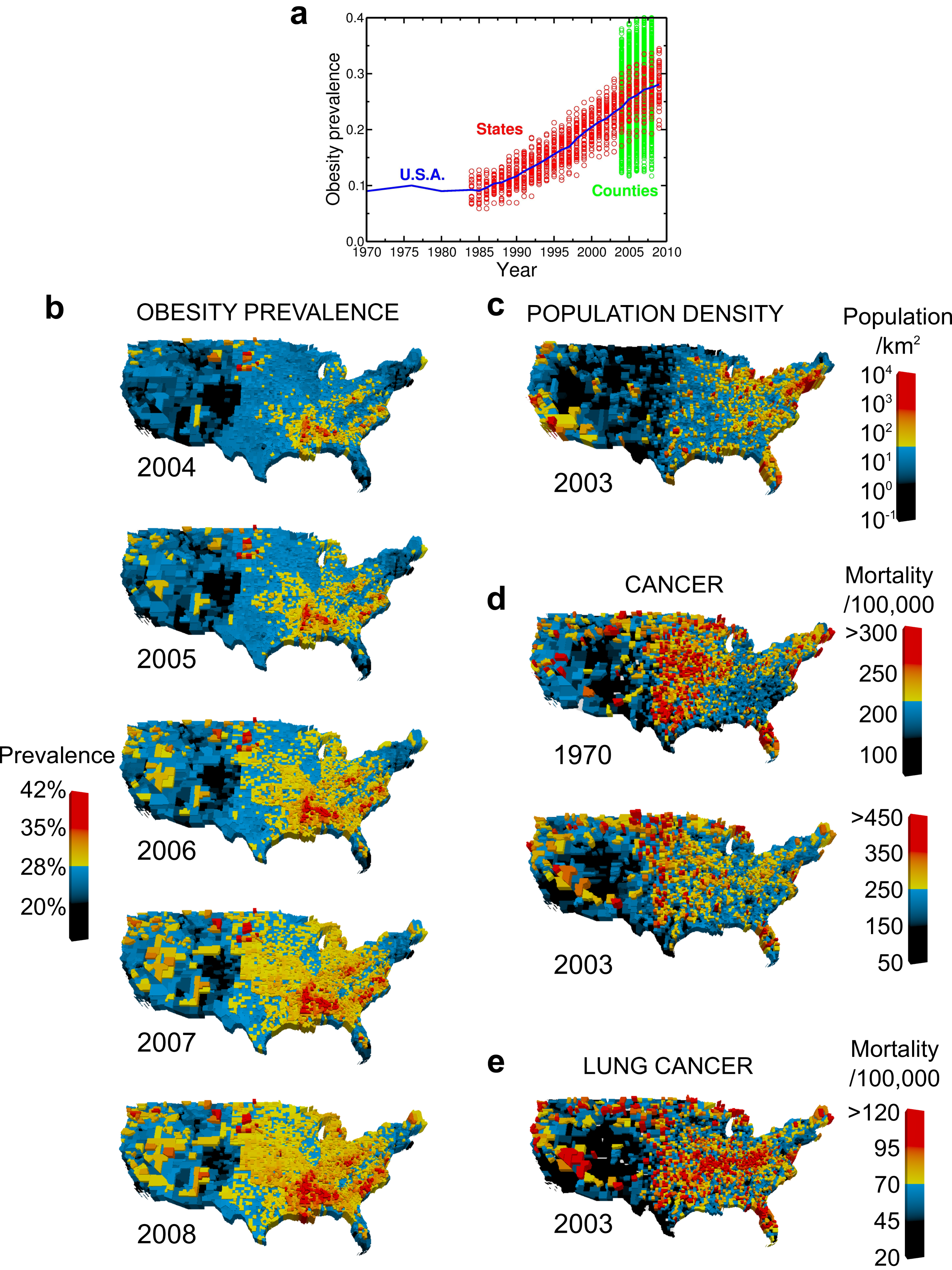
Figure 1: The obesity transition. a, CDC cdc provides an estimate of the number of obese adults, based on self-reported weight and height, country-wide since 1970 (blue line), at the state level from 1984 to 2009 (red symbols), and at the county level from 2004 to 2008 (green symbols). A transition is observed around 1980. We base our analysis on the micro-data at the county level. b, Map of the spatial spreading of obesity prevalence evidencing clustering dynamics. c, Map of the population density defined at the county level in 2003 showing correlated patterns albeit with less clustering than in obesity. d, Map of cancer mortality rates per county in 1970 and 2003 visualizing the transition from high correlations and clustering to weak correlation and more uniformity in 2003. e, Map of lung cancer mortality per county indicating large clustering properties similar to obesity.

The spatial map of obesity prevalence in the USA shows that neighboring areas tend to present similar percentages of obese population cdc forming spatial ‘obesity clusters’ schuurman ; michimi . The evolution of the spatial map of obesity from 2004 to 2008 at the county level (Fig. 1b) highlights the mechanism of cluster growth. Characterizing such geographical spreading presents a challenge to current theoretical physics frameworks of cluster dynamics stanley ; shlomo ; coniglio ; weinrib1 ; sona ; makse . The equal-time two-point correlation function, $C(r)$, determines the properties of such spatial arrangement by measuring the influence of an observable $x_{i}$ in county $i$ (e.g., in this study: adult population density, prevalence of obesity and diabetes, cancer mortality rates and economic activity) on another county at distance $r$ stanley :

$$C(r)\equiv\frac{1}{\sigma_{0}}\frac{\sum_{ij}(x_{i}-\overline{x})(x_{j}-\overline{x})\delta(r_{ij}-r)}{\sum_{ij}\delta(r_{ij}-r)}.$$ (1)

Here, $\overline{x}$ is the average over all $N=3,141$ counties in the USA, $\sigma_{0}=\sum_{i}(x_{i}-\overline{x})^{2}/N$ is the standard deviation, $r_{ij}$ is the euclidean distance between the geometrical center of counties $i$ and $j$. Large positive values of $C(r)$ reveal strong correlations, while negative values imply anti-correlations, i.e., two areas with opposed tendencies relative to the mean in obesity prevalence (analogous to two domains with opposite spins in a ferromagnet stanley ).

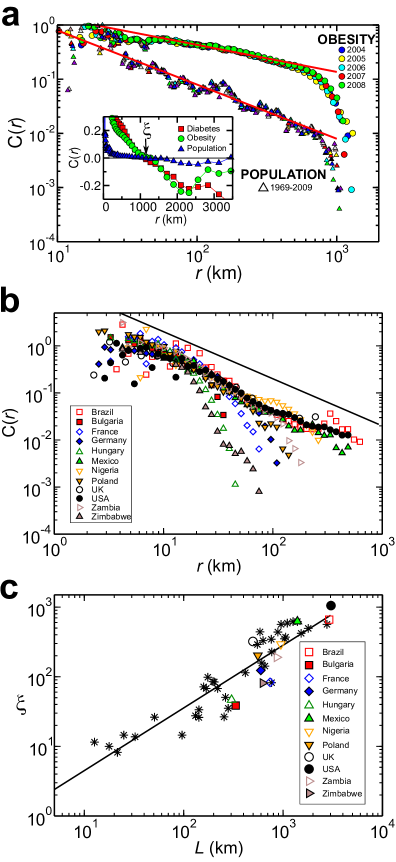
Figure 2: Long-range correlations in spreading phenomena. a, Correlation function, $C(r)$, averaged over counties at distance $r$ for population density from 1969-2009 and obesity prevalence from 2004-2008. The lines are fittings based on OLS regression analysis ols . The inset shows the correlation length at $C(\xi)=0$ and highlights the fact that $\xi$ is approximately the same for the population, obesity and diabetes prevalence (data for 2004). The inset also highlights the anticorrelations for $r>\xi$. b, Population density correlation function, $C(r)$ vs $r$, for different countries in 2009 as indicated. c, Correlation length $\xi$ vs linear country size $L$ for different countries. The symbols indicate the same countries as in Fig. 2b. The remaining star symbols are for other countries as indicated in Table 1. $L$ is the square root of the total area of the country.

Spatial correlations in any indicator ought to be referred to the natural correlations of population fluctuations (Fig. 1c). To this aim, we first calculate $C(r)$ for the population (adults $\geq$ 18 years) in USA counties, $p_{i}$, by using the density: $x_{i}=p_{i}/a_{i}$ in Eq. (1), where $a_{i}$ is the county area. Population density correlations show a slow fall-off with distance (Fig. 2a) described by a power-law up to a correlation length $\xi$:

$$C(r)\sim r^{-\gamma},\,\,\,\,\,r\lesssim\xi,$$ (2)

where $\gamma$ is the correlation exponent. Correlations become short-ranged when $\gamma\geq d$ ($d=2$ is the dimension of the map), and stronger as $\gamma$ decreases stanley ; shlomo . An Ordinary Least Squares (OLS) regression analysis ols on the population reveals the exponent $\gamma=1.01\pm 0.08$ (averaged over 1969-2009, Fig.  2a, error bars denote 95% confidence interval [CI]). The inset of Fig. 2a reveals a distance where correlations vanish, $C(\xi)=0$ with $\xi=1050$km, representing the average size of the correlated domains cavagna . As we increase $r$ larger than $\xi$, we consider correlations between areas in the East and West which are anti-correlated since $C(r)<0$ for $r>\xi$.

To determine whether population correlations are scale-free, we calculate $C(r)$ for geographical systems of different sizes using a high resolution grid of 2.5 arc-seconds, available for several countries from ciesin (Methods Section I.1). The resulting correlations (Fig. 2b) reveal the same picture as for the USA at the county-level (Fig. 2a), i.e., a power-law up to a correlation length. We then measure $\xi$ for every country, and investigate whether, as expected with the laws of critical phenomena stanley ; mora , it increases with the country size, $L$. Indeed, we obtain (Fig. 2c and Table 1),

$$\xi(L)\sim L^{\nu},$$ (3)

where $\nu=0.9\pm 0.1$ is the correlation length exponent stanley . This result implies that the fluctuations in human agglomerations are scale-free, i.e., the only length-scale in the system is set by its size and the correlation length become infinite when $L\to\infty$ stanley ; mora ; cavagna .

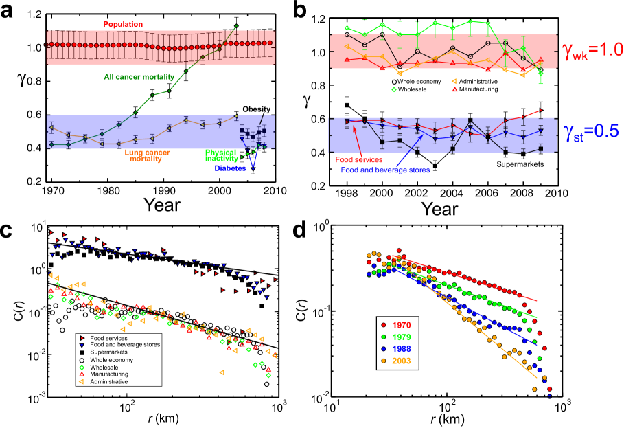
Figure 3: Correlation exponents. a, Temporal evolution of $\gamma$ for population distribution, obesity, diabetes, physical inactivity, all cancer mortality, and lung cancer mortality per county. The diagram displays the classes of strong correlations, $\gamma_{\rm st}=0.5$, and weak correlations, $\gamma_{\rm wk}=1$. Additionally, theory predicts $\gamma_{\rm rnd}\geq 2$ for uncorrelated systems. We did not observe any human activity or indicators whose correlations fall within this class, unless the data of different counties is shuffled. b, Evolution of $\gamma$ for different economic indicators describing the food industry, the whole economy and generic economic sectors as indicated. We quantify economic activity by the total number of employees of a given sector per county population. c, Correlation functions for the economic activities indicated in the figure. The plot shows the segregation of the data into two classes. The solid lines indicate $\gamma_{\rm wk}=1$ and $\gamma_{\rm st}=1/2$. d, Change in $C(r)$ for cancer mortality rates in the period 1970-2003.

We interpret any departure from $\gamma=1$ as a proxy of anomalous dynamics beyond the simple dynamics related to the population growth. When we calculate the spatial correlations of obesity prevalence ($s_{i}\equiv o_{i}/p_{i}$, $o_{i}$ is the number of obese adults in county $i$) in USA from 2004 to 2008 we also find long-range correlations (Fig. 2a). The crux of the matter is that the correlation exponent for obesity ($\gamma=0.50\pm 0.04$, averaged over 2004-2008) is smaller than that of the population, signaling anomalous growth. Since smaller exponents mean stronger correlations, the increase in obesity prevalence in a given place can eventually spread significantly further than expected from the population dynamics.

We also calculate fluctuations in variables which are known to be strongly related to obesity popkin ; cutler ; schuurman ; Mokdad_prevalence_of_obesity : diabetes and physical inactivity prevalence (fraction of adults per county who report no physical activity or exercise, see Methods Section I). The obtained $\gamma$ exponents are anomalous with similar values as in obesity (Fig. 3a). The system size dependence of $\xi$ for obesity and diabetes cannot be measured directly, since there is no available micro-data for other countries. However, we find that $\xi$ of obesity and diabetes in USA is very close to $\xi$ of the population distribution (inset of Fig. 2a). Assuming that the equality of the correlation lengths holds also for other countries, then obesity and diabetes should satisfy Eq. (3) as well.

The correlations in obesity are reminiscent of those in physical systems at a critical point of second-order phase transitions stanley ; mora ; cavagna . Physical systems away from criticality are uncorrelated and fluctuations in observables, e.g., magnetization in a ferromagnet or density in a fluid, decay faster than a power-law, e.g., exponentially stanley ; mora . Instead, long-range correlations appear at critical points of phase transitions where fluctuations are not independent and, as a consequence, fall-off more slowly. The existence of long-range correlations with $\gamma=0.5$— rather than the noncritical exponential decay— signals the emergence of strong critical fluctuations in obesity and diabetes spreading. The notion of criticality, initially developed for equilibrium systems stanley ; mora , has been successfully extended to explain a wide variety of dynamics away from equilibrium ranging from collective behaviour of bird cohorts, biological and social systems to city growth, just to name a few cavagna ; mora ; rozenfeld ; stanley3 . Its most important consequence is that it characterizes a system for which local details of interactions have a negligible influence in the global dynamics stanley ; mora . Following this framework, the clustering patterns of obesity are interpreted as the result of collective behaviors which are not merely the consequence of fluctuations of individual habits.

As a tentative way of addressing which elements of the economy may be related to the obesity spread, we calculate $\gamma$ in economic indicators which are thought to be involved in the rise in obesity swinburn ; nestle . Except for transient phenomena, all studied indicators yield exponents that fall around $\gamma_{\rm wk}=1$ or $\gamma_{\rm st}=1/2$, representing two universality classes of weak and strong correlations, respectively (Figs. 3a and b).

We begin by studying the correlations in the whole economy (measured through the number of employees of all economic sectors per county population, see Methods Section I). We find $\gamma$ close to $\gamma_{\rm wk}=1$ (over the period 1998-2009, Fig. 3b and c) suggesting that the whole economy inherits the correlations in the population. Generic sectors of the economy which are not believed to be drivers of obesity, e.g., wholesalers, administration, and manufacturing, also display $\gamma$ consistent with the population trend (Fig. 3b and c).

Interestingly, analysis of the spatial fluctuations in the economic activity of sectors associated to food production and sales (supermarkets, food and beverages stores and food services such as restaurants and bars) gives rise to the same anomalous value as obesity and diabetes ($\gamma_{\rm st}=1/2$, 1998-2009, Fig. 3b and c). Although these results cannot inform about the causality of these relations, they show that the scaling properties of the obesity patterns display a spatial coupling which is also expressed by the fluctuations of sectors of the economy related to food production.

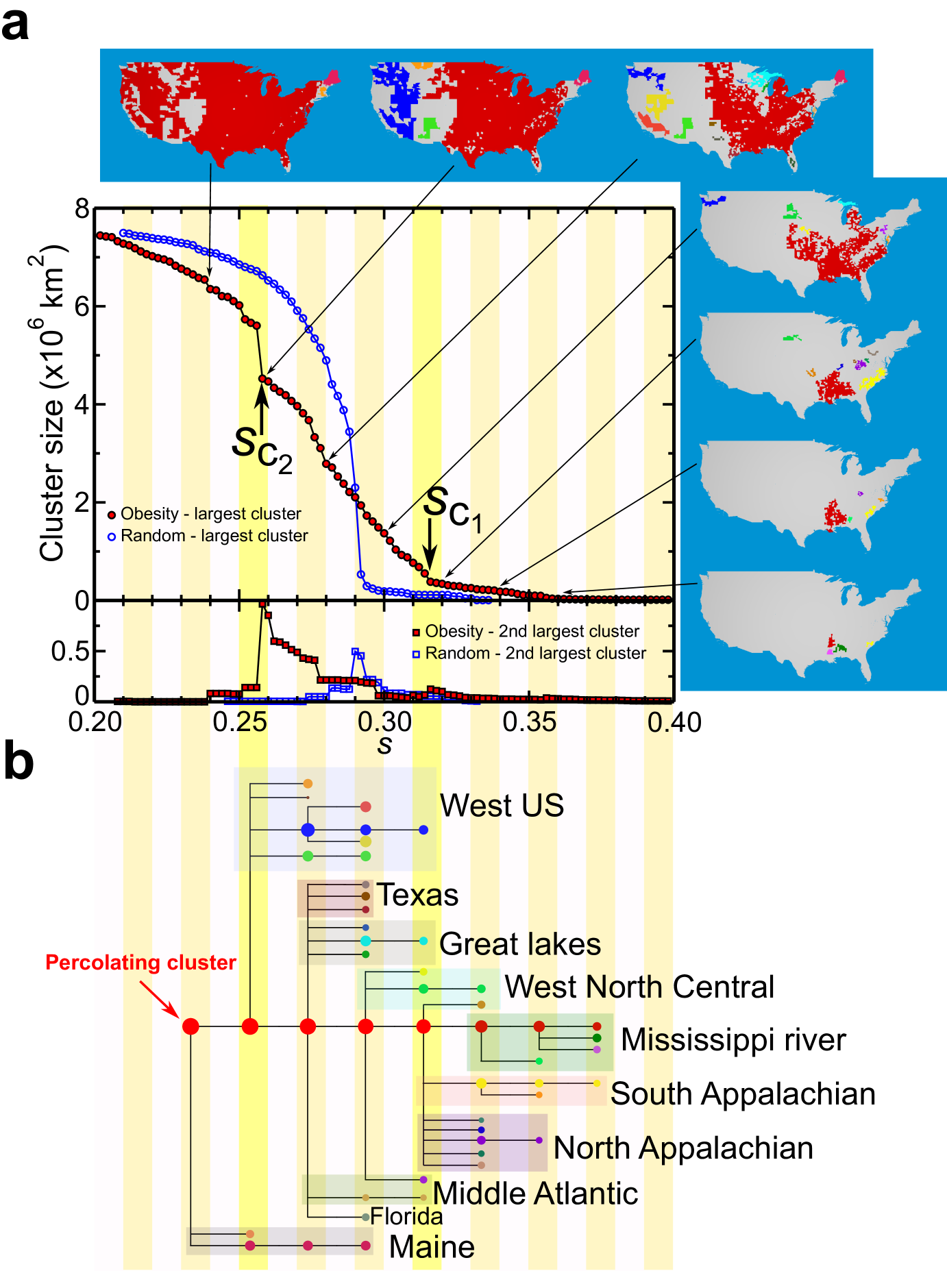
Figure 4: Percolation picture of obesity. a, Size of the largest component (circles) and second largest component (squares) as a function of the obesity prevalence threshold $s$ in 2008. As we lower $s$, the size of the largest component increases by absorbing smaller clusters. In many cases, this is done abruptly, indicating that whole clusters have been incorporated to the largest cluster as evidenced by the peaks in the second largest cluster and the jumps in the size of the largest clusters shlomo . We observe two main transitions at $s_{c_{1}}$ and $s_{c_{2}}$ in the real data (red) and a single percolation second-order transition in the randomized data (blue). The maps show the progression of the obesity clusters with at least 5 counties for a given $s$. b, Percolation tree representing the hierarchical formation, growth and merging of obesity clusters. Each dot represents a cluster at a given $s$ with a size proportional to the logarithm of the cluster’s area. Cluster colors follow Fig. 4a and we separate them by the indicated geographic regions. As we lower $s$ from right to left, regions of high obesity prevalence appear first in the tree. We notice the main percolating cluster starting in the lower Mississippi basin (red) at high $s$ and absorbing the other clusters until percolating through all US. In particular, we note the two main transitions at $s_{c_{1}}$, where it absorbs the two Appalachian clusters, and at $s_{c_{2}}$, where it absorbs the West US cluster.

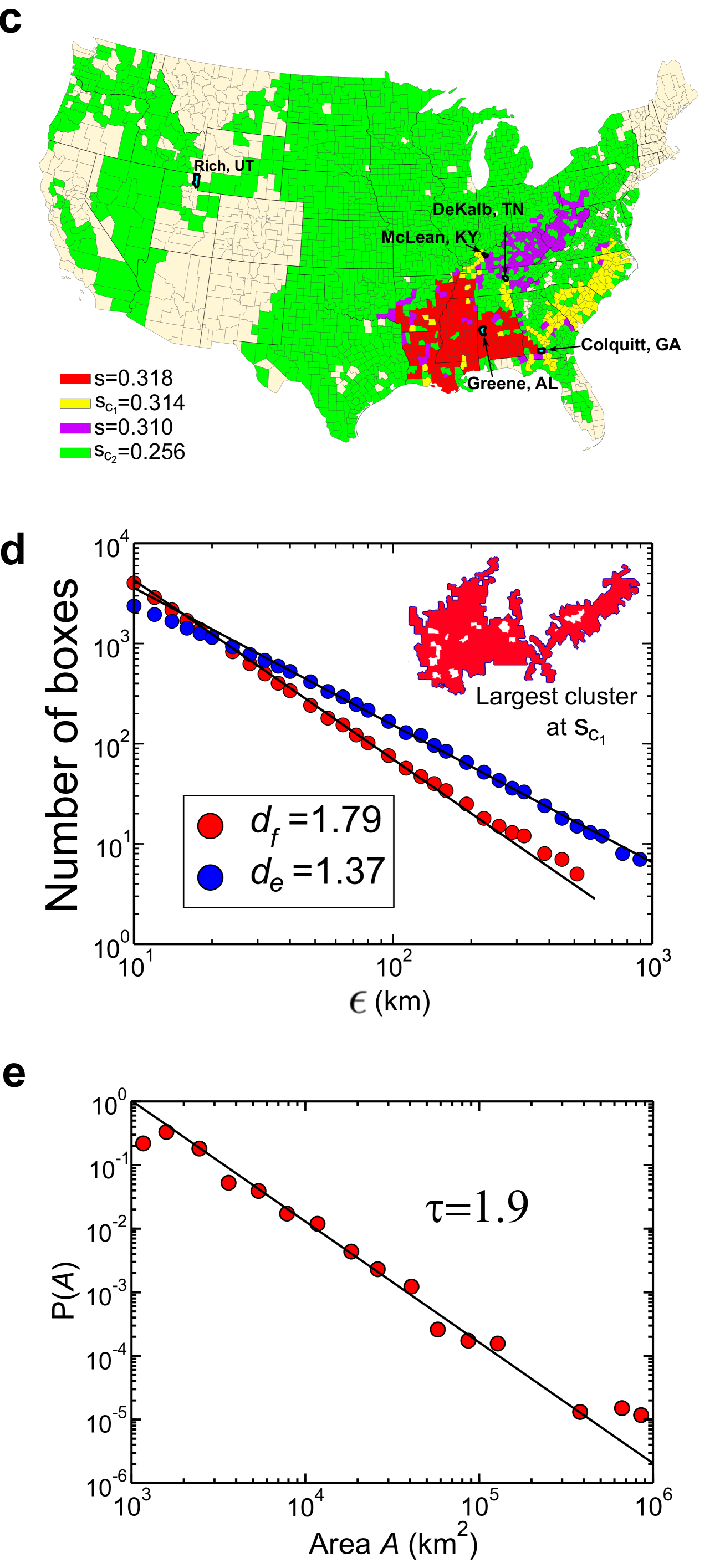
Figure 4: c, Detail of the evolution of obesity clusters near percolation as indicated. The map shows the shape of the first (red), second (yellow), and third (violet) clusters around $s_{c_{1}}$, and the largest (green) cluster at $s_{c_{2}}$, together with the location of the red bonds responsible for the transitions. The epicenter is Greene county, AL with 43.7% obesity prevalence. d, Box fractal dimension of percolating cluster in the inset measured by the number of boxes of size $\epsilon$ needed to cover the cluster: $N_{B}(\epsilon)\sim\epsilon^{-d_{f}}$, and fractal dimension of the boundary measured by the number of boxes needed to cover the hull: $N_{h}(\epsilon)\sim\epsilon^{-d_{e}}$. e, Probability distribution of the area of the obesity clusters, $P(A)\sim A^{-\tau}$, at percolation $s_{c_{1}}$ average from 2004-2008. This scaling law generalizes Zipf’s law rozenfeld from urban to obesity clusters.

It is of interest to study other health indicators for which active health policies have been devoted to control the rate of growth. We apply the correlation analysis to lung cancer mortality defined at the county level and compare with cancer mortality due to all types (Methods Section I). The spatial correlations of cancer mortality per county show an interesting transition in the late 70’s from anomalous strong correlations, $\gamma_{\rm st}=1/2$, to weak correlations, $\gamma_{\rm wk}=1$, (Fig. 3a and d). This transition is visualized in the different correlated patterns of cancer mortality in 1970 and 2003 in Fig. 1d, i.e., the clustering of the data is more profound in 1970, while in 2003 it spreads more uniformly. The current status of all-cancer mortality fluctuations is close to the natural one, inflicted by population correlation. Conversely, fluctuations in the mortality rate due to lung cancer from 1970 to 2003 have remained highly correlated and close to the obesity value, $\gamma_{\rm st}=1/2$ (Fig. 3a and 1e), while the other types of cancer have become less correlated. This is an interesting finding since, similarly to obesity, lung cancer prevalence is affected by a global factor (smoking) and has been growing rapidly during the studied period.

The most visible characteristic of correlations is the formation of spatial clusters of obesity prevalence. To quantitatively determine the geographical formation of obesity clusters, we implement a percolation analysis shlomo ; coniglio ; weinrib1 ; sona ; makse ; weinrib2 . The control parameter of the analysis is the obesity threshold, $s$. An obesity cluster is a maximally connected set of counties for which $s_{i}$ exceeds a given threshold $s$: $s_{i}\geq s$. By decreasing $s$, we monitor the progressive formation, growth and merging of obesity clusters.

In random uncorrelated percolation shlomo , small clusters would be formed in a spatially uniform way until a critical value, $s_{c}$, is reached, and an incipient cluster spans the entire system. Instead, when we analyze the obesity clusters we observe a more complex pattern exemplified in Fig. 4a and 4b for year 2008. At large $s$, the first cluster appears in the lower Mississippi basin (red in Fig. 4a) with epicenter in Greene county, AL. Upon decreasing $s$ to 0.32, new clusters are born including two spanning the South and North of the Appalachian Mountains, which acts as a geographical barrier separating the second and third largest clusters (yellow and violet in Fig. 4a, respectively). Further lowering $s$, we observe a percolation transition in which the Appalachian clusters merge with the Mississippi cluster. This point is revealed by a jump in the size of the largest component and a peak in the second largest component at $s_{c_{1}}=0.314$ (Fig. 4a) as features of a percolation transition shlomo . At $s_{c_{1}}$, three “red bonds” (McLean county, KY, DeKalb county, TN, and Colquitt county, GA) appear to connect the incipient largest cluster spanning the East of USA (see Fig. 4c and Methods Section II). As a comparison, when we randomize the obesity data by shuffling the values between counties, a single $s_{c}=0.29$ appears as a signature of a uncorrelated percolation process (blue symbols in Fig. 4a).

Obesity clusters in the West persist segregated from the main Eastern cluster avoiding a full-country percolation due to low-prevalence areas around Colorado state. Finally, the East and West clusters merge at $s_{c_{2}}=0.256$ by a red bond (Rich county, Utah) producing a second percolation transition; this time spanning the whole country (see Fig. 4a and c, where the whole spanning cluster is green, and Methods Section II). This cluster-merging process is a hierarchical percolation progression represented in the tree model in Fig. 4b.

To further inquire whether the spreading of obesity has the features of a physical system at the critical point, we examine the geometry and distribution of obesity clusters. For long-range correlated critical systems percolating through nearest neighbors in two dimensional maps, the geometrical structure shlomo ; sona ; makse gives rise to three critical exponents: the fractal dimension of the spanning cluster, $d_{f}$, the fractal dimension of the hull, $d_{e}$, and the cluster size distribution exponent, $\tau$, analogous to Zipf’s law rozenfeld (Methods Section III). For the percolating obesity cluster at $s_{c_{1}}$ displayed in the inset of Fig. 4d, we confirm critical scaling with exponents: $(d_{f},d_{e},\tau)=(1.79\pm 0.08,1.37\pm 0.06,1.9\pm 0.1)$ (Fig. 4d, e).

Taken together, these results show that obesity spreading behaves as a self-similar strongly-correlated critical system stanley ; mora . In particular, a note of caution has to be raised since, even if the highest prevalence of obesity is localized to the South and Appalachia, the scaling analysis indicates that the obesity problem is the same (self-similar) across all USA, including the lower prevalence areas.

Our results cannot establish a causal relation between obesity prevalence and economic indicators: whether fluctuations in the food economy may impact obesity or, instead, whether the food industry reacts to obesity demands. However, the comparative similarities of statistical properties of demographic and economical variables serves to identify possible candidates which shape the epidemic. Specifically, the observation of a common universality class in the fluctuations of obesity prevalence and economic activity of supermarkets, food stores and food services— which cluster in a different universality class than simple population dynamics— is in line with studies proposing that an important component of the rise of obesity is linked to the obesogenic environment hill ; obesogenic regulated by food market economies cutler ; swinburn ; nestle . This result is consistent with recent research that relates obesity with residential proximity to fast-food stores and restaurants christakis2 ; christakis3 . The present analysis based on clustering and critical fluctuations is a supplement to studies of association between people’s BMI and food’s environment based on covariance christakis2 ; christakis3 (Methods Section IV). We have detected potential candidates in the economy which relate to the spreading of obesity by showing the same universal fluctuation properties. These tentative relations ought to be corroborated by future intervention studies.

Acknowledgements: LKG and HAM are supported by NSF-0827508 Emerging Frontiers, and PB and MS by Human Frontiers Science Program. We are grateful to H. Nickerson for bringing our attention to this problem, and S. Alarcón-Díaz and D. Rybski for valuable discussions. We thank Epiwork, ARL and the Israel Science Foundation for support.

Methods

I Datasets

Obesity is determined through the Body Mass Index (BMI) which compares the weight and height of an individual via the formula weight(kg)/height(m²). A BMI value of 30 is considered the obesity threshold. Overweight but not obese is $25<$BMI$<30$, and underweight is BMI$<$18.5. Our main measure in this work is the adult obesity prevalence of a county, $s_{i}=o_{i}/p_{i}$, for a given year defined as the number of obese adults $o_{i}$ (BMI$>30$) in a county $i$ over the total number of adults in this county, $p_{i}$. We use the data from the USA Center for Disease Control (CDC) downloaded from cdc . CDC provides an estimate of the obesity country-wide since 1970, at the state level from 1984 to 2009, and at the county level from 2004 to 2008. The study of the correlation function $C(r)$ requires high resolution data. Therefore, we use data defined at the county level and restrict our study of obesity and diabetes to the available period 2004-2008. Other indicators are provided by different agencies at the county level for longer periods.

The datasets analyzed in this paper were obtained from the websites as indicated below. They can be downloaded as a single tar datafile from jamlab.org. The datasets consist of a list of populations and other indicators at specific counties in the USA at a given year. A graphical representation of the obesity data can be seen in Fig. 1b for USA from 2004 to 2008, where each point in the maps represents a data point of obesity prevalence directly extracted from the dataset.

The datasets that we use in our study have been collected from the following sources:

(a) Population.– US Census Bureau. We download a number of datasets at the county level from http://www.census.gov/support/USACdataDownloads.html

- For the population estimates we use the table PIN030. For the years 1969-2000 we use data supplied by BEA (Bureau of Economic Analysis) and for years 2000-2009 we use the file CO-EST2009-ALLDATA.csv from http://www.census.gov/popest/counties/files/CO-EST2009-ALLDATA.csv

(b) Health indicators.– Data downloaded from the Centers for Disease Control and Prevention (CDC).

http://apps.nccd.cdc.gov/DDT_STRS2/NationalDiabetesPrevalenceEstimates.aspx

The center provides county estimates between the years 2004-2008 for:

- Diagnosed diabetes in adults.

- Obesity prevalence in adults.

- Physical inactivity in adults.

The estimates for obesity and diabetes prevalence and leisure-time physical inactivity were derived by the CDC using data from the census and the Behavioral Risk Factor Surveillance System (BRFSS) for 2004, 2005, 2006, 2007 and 2008. BRFSS is an ongoing, state-based, random-digit-dialed telephone survey of the U.S. civilian, non-institutionalized population aged 18 years and older. The analysis provided by the BRFSS is based on self-reported data, and estimates are age-adjusted on the basis of the 2000 US standard population. Full information about the methodology can be obtained at http://www.cdc.gov/diabetes/statistics.

(c) Economic indicators.– We download data for economic activity through http://www.census.gov/econ/. The economic activity of each sector is measured as the total number of employees in this sector per county in a given year normalized by the population of the county. The North American Industry Classification System (NAICS) (http://www.census.gov/epcd/naics02/naicod02.htm) assigns hierarchically a number based on the particular economy sector. The NAICS is the standard used by US statistical agencies in classifying business establishments across the US business economy.

In this study we have used the following economic sectors with their corresponding NAICS:

• Whole economy. Entire output of all economic sectors combined including all NAICS codes.

• 31. Manufacturing. Broad economic sector from textiles, to construction materials, iron, machines, etc.

• 42. Wholesale trade. Very broad sector including merchants wholesalers, motors, furniture, durable goods, etc.

• 56. Administrative jobs and support services.

• 445. Food and beverage stores. Including all the food sectors, from supermarkets, fish, vegetables meat markets, to restaurants and bars and other services to the food industry.

• 44511. Supermarkets and other grocery (except convenience) stores. This is a subsection of NAICS 445.

• 722. Food services and drinking places. A sub-sector of NAICS 72 which includes restaurants, cafeterias, snacks and nonalcoholic beverage bars, caterers, bars and drinking places (alcoholic beverages).

(d) Mortality rates.– We use data from the National Cancer Institute SEER, Surveillance Epidemiology and End Results downloaded from http://seer.cancer.gov/data/

The Institute provides mortality data from 1970 to 2003, aggregated every three years. We analyze the mortality of a specific form of cancer per county normalized by the population of the county. Here, we use mortality data for the following causes of death:

- All cancer, independently of type.

- Lung cancer.

I.1 Gridded data of population from CIESIN

We take advantage of the available data of population distribution around the globe defined in a square grid of 2.5 arc-seconds obtained from ciesin . This data allows to study the correlation functions of the population distribution for many countries. By using this data we are able to test the system size dependence of our results. We find that the correlation length $\xi$ is proportional to the linear size of the country, $L$. The linear size is calculated as Total Area = $L^{2}$. We find that the correlation scales with the system size as discussed in the text. For instance, for the USA population distribution we find $\xi=1050$km, while a smaller country like UK has $\xi=321$ km.

Table 1 shows a list of countries used in Figs. 2b and c to determine the correlation length $\xi$ of the correlation function of population density.

II Evolution of obesity clusters near percolation

The shape of the main obesity clusters and location of the red bonds and obesity epicenter are depicted in Fig. 4c overlayed with a US map showing the boundaries of states and counties. Figure 4c shows the obesity clusters obtained at $s=0.318$, $s_{c_{1}}=0.314$, $s=0.310$, and $s_{c_{2}}=0.256$, depicting the process of percolation. At $s=0.318$, we plot the largest red cluster which is seen in the lower Mississippi basin. The highest obesity prevalence is in Greene county, AL, which acts as the epicenter of the epidemic. At $s_{c_{1}}$, we plot in yellow the second largest cluster in the Atlantic region south of the Appalachian Mountains, and at $s=0.310$ we plot the third largest cluster (violet), which appears north of the Appalachian Mountains. We mark with black the three red bonds that make the Mississippi cluster to grow abruptly by absorbing the clusters in the Appalachian range. The red bonds are DeKalb county, TN, McLean county, KY, and Colquitt county, GA. This transition is reflected in the jump in the size of the largest cluster in Fig. 4a. The same process is observed in the second percolation transition at $s_{c_{2}}$, when the red bond, Rich county, UT, joins the Eastern and Western clusters for a whole-country percolation.

III Scaling exponents of percolation clusters

The scaling properties characterizing the geometry and distribution of clusters at percolation are shlomo :

(i) The scaling of the number of boxes $N_{B}$ to cover the infinite spanning cluster versus the size of the boxes $\epsilon$:

$$N_{B}(\epsilon)\sim\epsilon^{-d_{f}},$$ (4)

defining the fractal dimension of the spanning cluster, $d_{f}$.

(ii) The number of boxes, $N_{h}$, of size $\epsilon$ covering the perimeter of the infinite cluster:

$$N_{h}(\epsilon)\sim\epsilon^{-d_{e}},$$ (5)

defining the hull fractal dimension, $d_{e}$.

(iii) The probability distribution of the area of clusters at percolation:

$$P(A)\sim A^{-\tau},$$ (6)

characterized by the critical exponent $\tau$. Additionally, there is a scaling relation between the fractal dimension and the cluster distribution exponent shlomo : $\tau=1+2/d_{f}.$

The exponents $(d_{f},d_{e},\tau)$ for percolation with long-range correlations have been calculated numerically in sona ; makse as a function of the correlation exponent $\gamma$ using standard percolation analysis. There exist also a theoretical prediction based on Renormalization Group in weinrib1 for the correlation length exponent. The values of $(d_{f},d_{e},\tau)$ for the obesity clusters at the first percolation transition, $s_{c_{1}}$, are reported in the main text. A direct computer simulations of long-range percolation sona ; makse for $\gamma=0.5$ finds the values of the three geometric exponents to be $(d_{f},d_{e},\tau)=(1.9\pm 0.1,1.39\pm 0.03,2.05\pm 0.08)$, consistent with those reported here.

We notice that the exponent $\tau$ is expected to be larger than 2. This is due to mass conversation, assuming that the power-law Eq. (6) extends to infinity at percolation in a infinite system size. The fact that we find a value slightly smaller than 2 for the obesity clusters, might be due to a finite size effect. We also notice that the values of the exponents obtained from correlated percolation at $\gamma=0.5$ are not too far from those of uncorrelated percolation sona . Therefore, the values of the exponents may not be enough to precisely compare the obesity clusters with long-range percolation clusters. However, they serve as an indication that the obesity clusters have the geometrical properties of clusters at a critical point, such as scaling behavior. Furthermore, it could be possible that long-range correlated percolation may capture only part of the dynamics of the clustering epidemic. It could be, for instance, that higher order correlations, beyond the two-point correlation captured by $C(r)$, are also relevant in determining the value of the exponents. In this case, our analysis should be supplemented by studies of $n-$point correlation functions, beyond $C(r)$.

Table 1: List of countries used to calculate the correlation length, $\xi$, from the correlation function of the population density. Data is obtained from ciesin . $L$ is calculated as the square root of the total area of the country.

Country name	$L$ (km)	$\xi$ (km)
Liechtenstein	12.65	11.5
Malta	17.75	10
Andorra	21.54	8.2
Bahrain	24.96	14.5
Hong-Kong	32.46	13.7
Luxembourg	50.86	26.24
Cyprus	96.29	14.5
Kuwait	131.37	27.5
Slovenia	142.21	26
El Salvador	142.40	33.5
Burundi	158.83	71.5
Albania	168.36	67.8
Belgium	174.79	98.3
Switzerland	197.42	85
Netherlands	203.38	84
Dominican Republic	219.29	67.7
Lithuania	254.94	26.5
Ireland	263.58	50.5
Czech Republic	280.38	35.2
Hungary	303.39	46.5
Bulgaria	333.63	38.5
Uruguay	417.11	114
United Kingdom	497.18	321
Oman	551.53	290
Poland	557.85	202

Table 2: Continuation

Country name	$L$ (km)	$\xi$ (km)
Congo	585.86	440
Germany	596.68	123
Japan	609.68	157
Zimbabwe	623.74	81
Paraguay	629.19	330
Iraq	656.18	142
France	739.68	83
Kenya	761.33	345
Ukraine	767.08	82
Madagascar	770.04	227
Zambia	863.317	190
Pakistan	886.183	438
Nigeria	950.913	293
Venezuela	954.756	565
Bolivia	1034.09	350
Ethiopia	1060.05	370
South Africa	1103.47	588
Iran	1261.09	618
Saudi Arabia	1392.42	618
Mexico	1393.92	622
Congo Democratic Republic	1520.99	420
India	1791.57	495
Australia	2763.09	565
Brazil	2912.11	660
United States of America	3034.92	1050

IV Covariance

Our approach supplements covariance analysis christakis2 ; christakis3 . Instead, we use physics concepts to shed a different view on the spreading of epidemics. Our approach can be extended to the study of the geographical spreading of any epidemic: from diabetes and lung cancer, to the spreading of viruses or real states bubbles, where the spatial spreading plays an important role.

Population correlations are naturally inherited by all demographic observables. Even variables whose incidence varies randomly from county to county would exhibit spatial correlations in their absolute values, simply because its number increases in more populated counties and population locations are correlated. Indeed, the absolute number of obese adults per county is directly proportional to the population of the county [Bettencourt, L. M. A., et al. Growth, innovation, scaling, and the pace of life in cities. Proc. Natl. Acad. Sci. USA 104, 7301-7306 (2007)]. Our aim is to measure spatial fluctuations on the frequency of incidence, independent of population agglomeration. Thus, spatial correlations of all indicators ought to be calculated on the density defined, in the case of obesity, as $s_{i}=o_{i}/p_{i}$ rather than on the absolute number of obese people, $o_{i}$, itself. The spatial correlations of the fluctuations of $s_{i}$ from the global average captures the collective behavior expressed in the power-law described in Eq. (2).

References

- (1) World Health Organization. Obesity: Preventing and managing the global epidemic. WHO Obesity Technical Report Series 894 (World Health Organization Geneva, Switzerland, 2000).
- (2) Butland, B. et al., Foresight tackling obesities: future choices-project report, 2nd edn. London: Government Office for Science (2007).
- (3) Hill, J. O. & Peters J. C. Environmental contributions to the obesity epidemic. Science 280, 1371-1374 (1998).
- (4) Swinburn, B. A., Sacks, G., Hall, K. D., McPherson, K., Finegood, D. T., Moodie, M. L. & Gortmaker, S. L. The global obesity pandemic: shaped by global drivers and local environments. Lancet 378, 804-814 (2011).
- (5) Nestle, M. Food politics: How the food industry influences nutrition and health. (University of California Press, revised edition, 2007).
- (6) Christakis, N. A. & Fowler, J. H. The spread of obesity in a large social network over 32 years. N. Engl. J. Med. 357, 370-379 (2007).
- (7) Block, J., Christakis, N.A., O’Malley, A.J. & Subramanian, S. Proximity to food establishments and body mass index in the Framingham Heart Study Offspring Cohort over 30 years. American Journal of Epidemiology 174, 1108-1114 (2011).
- (8) Caballero, B. & Popkin, B. M., editors. The Nutrition transition: diet and disease in the developing world (Academic Press, 2002).
- (9) Cutler, D. M., Glaeser, E. L. & Shapiro J. M. Why have Americans become more obese? J. Econ. Perspect. 17, 93-118 (2003).
- (10) Haslam D. W. & James, W. P. Obesity. Lancet 366, 1197-1209 (2005).
- (11) Department of Health and Human Services (USA). Healthy People 2010: understanding and improving health. Conference edition. (Washington, Government Printing Office, 2000).
- (12) Schuurman, N., Peters, P. A. & Oliver, L. N. Are obesity and physical activity clustered? A spatial analysis linked to residential density. Obesity 17, 2202-2209 (2009).
- (13) Michimi, A. & Wimberly, M. C. Spatial patterns of obesity and associated risk factors in the conterminous U.S. Am. J. Prev. Med. 39, e1-e12 (2010).
- (14) Behavioral Risk Factor Surveillance System Survey Data. Atlanta, Georgia: U.S. Department of Health and Human Services, Centers for Disease Control and Prevention. http://apps.nccd.cdc.gov/DDT_STRS2/NationalDiabetesPrevalenceEstimates.aspx
- (15) Stanley, H. E. Introduction to phase transitions and critical phenomena. (Oxford University Press, Oxford, 1971).
- (16) Bunde, A. & Havlin, S. (editors). Fractals and Disordered Systems (Springer-Verlag, Heidelberg, 2nd edition, 1996).
- (17) Coniglio, A., Nappi, C., Russo, L. & Peruggi, F. J. Phys. A 10, 205-209 (1977)
- (18) Weinrib, A. Long-range correlated percolation. Phys. Rev. B 29, 387-395 (1984).
- (19) Prakash, S., Havlin, S., Schwartz, M. & Stanley, H. E. Structural and dynamical properties of long-range correlated percolation. Phys. Rev. A 46, R1724-1727 (1992).
- (20) Makse, H. A., Havlin, S. & Stanley, H. E. Modelling urban growth patterns. Nature 377, 608-612 (1995).
- (21) Mora, T. & Bialek, W. Are biological systems poised at criticality? J. Stat. Phys 144, 268-302 (2011).
- (22) Montogomery, D. C., Peck, E. A. Introduction to linear regression analysis (Wiley, New York, 1992).
- (23) Cavagna, A., Cimarelli, A., Giardina, I., Parisi, G., Santagati, R. Stefanini, F. & Viale, M. Scale-free correlations in starling flocks. Proc. Natl. Acad. Sci. USA 107, 11865-11870 (2010).
- (24) Center for International Earth Science Information Network (CIESIN), Columbia University; and Centro Internacional de Agricultura Tropical (CIAT). 2005. Gridded Population of the World, Version 3 (GPWv3). Palisades, NY: Socioeconomic Data and Applications Center (SEDAC), Columbia University. Available at http://sedac.ciesin.columbia.edu/gpw.
- (25) Mokdad, A. H. et al., Prevalence of obesity, diabetes, and obesity-related health risk factors, 2001. JAMA 289, 76-79 (2003).
- (26) Rozenfeld, H. D., Rybski, D., Gabaix, X. & Makse, H. A. The area and population of cities: New insights from a different perspective on cities. American Economic Review 101, 560-580 (2011).
- (27) Stanley, H. E., et al. Scale-invariant correlations in the biological and social sciences. Phil. Mag. Part B 77, 1373-1388 (1998).
- (28) Weinrib, A. & Halperin, B. I. Critical phenomena in systems with long-range-correlated quenched disorder. Phys. Rev. B 27, 413-427 (1983).
- (29) Swinburn, B. & Figger, G. Preventive strategies against weight gain and obesity. Obesity Reviews 3, 289-301 (2002).
- (30) Chang, V. W. & Christakis, N.A. Income Inequality and Weight Status in U.S. Metropolitan Areas. Social Science and Medicine 61, 83-96 (2005).