Probability-preserving evolution in a non-Hermitian two-band model

Abstract

A non-Hermitian $\mathcal{PT}$-symmetric system can have full real spectrum but does not ensure probability preserving time evolution, in contrast to that of a Hermitian system. We present a non-Hermitian two-band model, which is comprised of dimerized hopping terms and staggered imaginary on-site potentials, and study the dynamics in the exact $\mathcal{PT}$-symmetric phase based on the exact solution. It is shown that an initial state, which does not involve two equal-momentum-vector eigenstates in different bands, obeys perfectly probability-preserving time evolution in terms of the Dirac inner product. Beyond this constriction, the quasi-Hermitian dynamical behaviors, such as non-spreading propagation and fractional revival of a Gaussian wave packet, are also observed.

I Introduction

Hermiticity of the Hamiltonian as the fundamental postulate in quantum mechanics guarantees the real eigenvalues and the conservation of probability. However, the recent discovery of Bender and Boettcher showed that Hermiticity of the Hamiltonian is not essential for a real spectrum bender . It has been proved that a non-Hermitian $\mathcal{PT}$-symmetric Hamiltonian can have real spectrum AM43 ; mosta1 ; mosta2 . Based on a time-independent inner product with a positive-definite norm, a new class of complex quantum theories having positive probabilities and unitary time evolution is established. The Hermitian and the non-Hermitian Hamiltonians seem to describe two parallel worlds, and much effort has been devoted to the connection between them bender ; AM43 ; mosta1 ; mosta2 ; Ahmed ; Berry ; Heiss ; Jones ; Muga ; Bender02 ; BenderRPP ; Tateo ; AMIJGMMP ; MZnojil ; Bender03 ; Bender04 .

One of the ways of connecting a pseudo-Hermitian Hamiltonian with its Hermitian counterpart is the metric-operator theory outlined in mosta2 , providing a mapping between them. However, the obtained equivalent Hermitian Hamiltonian is usually quite complicated mosta2 ; jin . Alternative ways, such as the interpretation of the non-Hermitian systems in the frameworks of scattering and quantum phase transition, have been investigated jin2 ; JLPRA83 ; JLJPA44 ; GLG2 ; MoiseyevBook .

In this work, we investigate the dynamics of a $\mathcal{PT}$-symmetric pseudo-Hermitian Hamiltonian in the context of unbroken $\mathcal{PT}$ symmetry. We consider an exactly solvable non-Hermitian $\mathcal{PT}$ model. It is a two-band tight-binding ring, with the non-Hermiticity arising from staggered imaginary potentials. It has been shown that such potentials can be realized in the realm of optics through a judicious inclusion of index guiding and gain/loss regions JPA38.171 ; PRL103904 ; PRL030402 ; OL2632 . Recently, it was reported that the most salient character of the pseudo-Hermitian Hamiltonian, which is the $\mathcal{PT}$ symmetry breaking, was observed experimentally AGuo ; Ruter . Nevertheless, the reality of the spectrum is not the unique common feature for the pseudo-Hermitian and the Hermitian systems in some cases. In Ref. LJin2012 it is pointed out that some non-Hermitian scattering centers, which consist of two Hermitian clusters with anti-Hermitian couplings between them, can act as Hermitian scattering centers, i.e. the S-matrix is unitary, or the Dirac probability current is conserved. The goal of the present work is to show the dynamical similarity between a non-Hermitian system and a Hermitian one. Intuitively, closely localized gain and loss potentials may be balanced with each other, or equivalently, the temporal and spatial large-scale dynamics should be probability preserving. The Dirac inner product can be measured in an universal manner in experiments, hence it is of central importance to most practical physical problems. In this work we aim at investigating the dynamical behavior in terms of the Dirac inner product. Within the unbroken $\mathcal{PT}$-symmetric region, the eigenfunctions with different $k$ are orthogonal spontaneously in terms of the Dirac inner product. This feature ensures the probability-preserving evolution of a state, which involves only one or two subbands with different $k$. In this sense, the non-Hermitian Hamiltonian acts as a Hermitian one without employing the biorthogonal inner product. We also provide some illustrative simulations to show the occurrence of the fractional revivals and the slowly spreading of a wave packet. It shows that for certain special models, the non-Hermitian and Hermitian Hamiltonians can describe the same physics within a certain energy range.

This paper is organized as follows. In Sec. II, we present a non-Hermitian $\mathcal{PT}$-symmetric two-band model and its exact solution. In Sec. III, we investigate the Hermitian counterpart of this model. In Sec. IV, we show the quasi-canonical commutation relations and the quasi-Hermitian dynamics. In Sec. V, we demonstrate the results for the system approaching to the exceptional point. Sec. VI is the summary and discussion.

II Model and solutions

We consider a two-band model described by a non-Hermitian Hamiltonian $H$. It is a tight-binding ring with the Peierls distortions between nearest-neighboring sites and the additional staggered imaginary on-site potentials, which can be written as follows

$$H = -J\sum_{l=1}^{2N}\left[1+\left(-1\right)^{l}\delta\right]\left(a_{l}^{\dagger}a_{l+1}+\mathrm{H.c.}\right)$$ (1)

$$+i\gamma\sum_{l}\left(-1\right)^{l}a_{l}^{\dagger}a_{l},$$

where $a_{l}^{\dagger}$ is the creation operator of a boson (or a fermion) at the $l$th site, with the periodic boundary condition $a_{2N+1}=a_{1}$. The hopping strengths, the distortion factor and the alternating imaginary potential magnitude are denoted by $J$, $\delta$ and $\gamma$ ($\gamma>0$), respectively. A sketch of the lattice is shown in Fig. 1. In the absence of the staggered potentials or the Peierls distortion (with real potentials), it is a standard two-band model and is employed to be a gapped data bus for quantum state transfer YSJCP ; HMXEPL ; ChenB . It is a $\mathcal{PT}$-symmetric model with respect to an arbitrary diameter axis. Here, without loss of generality, we define the action of time reversal and parity in such a ring system as follows. While the time reversal operation $\mathcal{T}$ is such that $\mathcal{T}i\mathcal{T}=-i$, the effect of the parity is such that $\mathcal{P}a_{l}^{\dagger}\mathcal{P}=a_{2N+1-l}^{\dagger}$. Applying operators $\mathcal{P}$ and $\mathcal{T}$ on the Hamiltonian (1), one has $\left[\mathcal{T},H\right]\neq 0$ and $\left[\mathcal{P},H\right]\neq 0$, but $\left[\mathcal{PT},H\right]=0$. According to the non-Hermitian quantum theory, such a Hamiltonian may have fully real spectrum when appropriate parameters are taken. In the following, we will diagonalize this Hamiltonian and show that it has fully real spectrum.

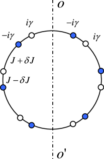
Figure 1: (Color online) Schematic illustration of the Peierls tight-binging ring with staggered imaginary potentials (solid and empty circles). It is $\mathcal{PT}$-symmetric with respect to the $OO^{\prime}$ axis and invariant under the translation.

Beyond the $\mathcal{PT}$ symmetry, $H$ is invariant under the translational transformation. Then taking the Fourier transform

$$A_{k} = \frac{1}{\sqrt{N}}\sum_{l=1}^{N}e^{-ikl}a_{2l-1},$$

$$B_{k} = \frac{1}{\sqrt{N}}\sum_{l=1}^{N}e^{-ikl}a_{2l},$$ (2)

where $k=2\pi n/N$, $n\in\left[0,N-1\right]$ is the momentum, the original Hamiltonian can be expressed as

$$H=\sum_{k}H_{k}$$ (3)

with

$$H_{k} = -J\left[\left(1-d+\left(1+d\right)e^{-ik}\right)A_{k}^{\dagger}B_{k}+\mathrm{H.c.}\right]$$

$$-i\gamma\left(A_{k}^{\dagger}A_{k}-B_{k}^{\dagger}B_{k}\right).$$

Here $A_{k}^{\dagger}$ and $B_{k}^{\dagger}$ are two kinds of creation operators of bosons (or fermions), resulting $\left[H_{k},H_{k^{\prime}}\right]=0$. The operator $H_{k}$ is non-Hermitian and can be readily written as

$$H_{k}=-\epsilon_{k}\left(\bar{\alpha}_{k}\alpha_{k}-\bar{\beta}_{k}\beta_{k}\right),$$ (4)

by applying the linear transformation

$$\alpha_{k} = \mu_{k}A_{k}+\nu_{k}B_{k},$$

$$\beta_{k} = -\bar{\nu}_{k}A_{k}+\bar{\mu}_{k}B_{k},$$ (5)

and

$$\bar{\alpha}_{k} = \bar{\mu}_{k}A_{k}^{\dagger}+\bar{\nu}_{k}B_{k}^{\dagger},$$

$$\bar{\beta}_{k} = -\nu_{k}A_{k}^{\dagger}+\mu_{k}B_{k}^{\dagger},$$ (6)

where the spectrum is given by

$$\epsilon_{k}=2J\sqrt{\left(1-\delta^{2}\right)\cos^{2}\left(\frac{k}{2}\right)+\delta^{2}-\left(\frac{\gamma}{2J}\right)^{2}},$$ (7)

and

$$\mu_{k}= \cos\theta_{k}e^{i\frac{\phi_{k}}{2}},\ \bar{\mu}_{k}= \cos\theta_{k}e^{-i\frac{\phi_{k}}{2}},$$

$$\nu_{k}= \sin\theta_{k}e^{-i\frac{\phi_{k}}{2}},\ \bar{\nu}_{k}= \sin\theta_{k}e^{i\frac{\phi_{k}}{2}},$$ (8)

where $\theta_{k}$ and $\phi_{k}$ are

$$\phi_{k} = \left\{\begin{aligned} &\frac{k}{2}+\tan^{-1}\left[\delta\tan\left(\frac{k}{2}\right)\right],&k<\pi,\\ &\frac{k}{2}+\tan^{-1}\left[\delta\tan\left(\frac{k}{2}\right)\right]+\pi,&k\geq\pi,\end{aligned}\right.$$

$$\theta_{k} = \cos^{-1}\left[\sqrt{\left(1+i\lambda_{k}\right)/2}\right],$$

with $\phi_{k}\in\left[0,2\pi\right]$, $\delta>0$ and $\lambda_{k}=\gamma/\epsilon_{k}$.

The non-Hermitian operator $H_{k}$ in Eq. (4) is in diagonal form, since $\alpha_{k}$, $\bar{\alpha}_{k}$, $\beta_{k}$, and $\bar{\beta}_{k}$ are canonical conjugate operators, obeying the canonical commutation relations

$$\left[\alpha_{k},\bar{\alpha}_{k^{\prime}}\right]_{\pm}= \left[\beta_{k},\bar{\beta}_{k^{\prime}}\right]_{\pm} =\delta_{kk^{\prime}},$$

$$\left[\alpha_{k},\alpha_{k^{\prime}}\right]_{\pm}= \left[\beta_{k},\beta_{k^{\prime}}\right]_{\pm} =0,$$

$$\left[\bar{\alpha}_{k},\bar{\alpha}_{k^{\prime}}\right]_{\pm}= \left[\bar{\beta}_{k},\bar{\beta}_{k^{\prime}}\right]_{\pm} =0,$$ (9)

$$\left[\alpha_{k},\bar{\beta}_{k^{\prime}}\right]_{\pm}= \left[\bar{\alpha}_{k},\bar{\beta}_{k^{\prime}}\right]_{\pm} =0,$$

$$\left[\alpha_{k},\beta_{k^{\prime}}\right]_{\pm}= \left[\bar{\alpha}_{k},\beta_{k^{\prime}}\right]_{\pm} =0.$$

Therefore, the original Hamiltonian (1) is diagonalized. The method employed here is similar to that for the Hermitian two-band models PRB2099 ; HMXEPL ; ChenB . Nevertheless, the transformation in Eqs. (5) and (6) is no longer unitary under the Dirac inner product, since the canonical conjugate pairs appearing in Eq. (9) are not simply defined by the Hermitian conjugate operation, i.e. $\bar{\alpha}_{k}\neq\alpha_{k}^{\dagger}$ and $\bar{\beta}_{k}\neq\beta_{k}^{\dagger}$, which is crucial in this work.

We note that the spectrum $\epsilon_{k}$ consists of two branches separated by an energy gap

$$\Delta=\sqrt{4J^{2}\delta^{2}-\gamma^{2}}.$$ (10)

Obviously, it displays a full real spectrum within the region of $4J^{2}\delta^{2}\geq\gamma^{2}$. Beyond this region, the imaginary eigenvalues appears and the $\mathcal{PT}$ symmetry of the corresponding eigenfunction is broken simultaneously according to the non-Hermitian quantum theory. Interestingly, it occurs independently on the size of the lattice. Notice that, when the onset of the $\mathcal{PT}$ symmetry breaking begins, the band gap vanishes, which is similar to that in a Hermitian two-band model. However, the dimerization still exists ($\delta\neq 0$), when the gap vanishes in this non-Hermitian model. In the next section, the further relationship between a non-Hermitian and a Hermitian two band models will be discussed.

III Hermitian counterpart

In this section, we would like to construct the equivalent Hermitian counterpart of the non-Hermitian model Eq. (1), which is a typical topic in the non-Hermitian quantum theory. In general, this can be done in the framework of metric-operator theory mosta1 ; mosta2 . Nevertheless, for the present model one can achieve this goal in a more direct way. This is due to the fact that the spectrum $\epsilon_{k}$ has an evident physical meaning. To demonstrate this point, we consider the model of a Peierls distorted tight-binding ring with staggered real potentials. The Hamiltonian can be written as

$$H_{\mathrm{e}} = -J_{\mathrm{e}}\sum_{l=1}^{2N}\left[1+\left(-1\right)^{l}\delta_{\mathrm{e}}\right]\left(b_{l}^{\dagger}b_{l+1}+\mathrm{H.c.}\right)$$ (11)

$$+V_{\mathrm{e}}\sum_{l}\left(-1\right)^{l}b_{l}^{\dagger}b_{l},$$

where $b_{l}^{\dagger}$ is the creation operator of a boson (or a fermion) at the $l$th site, with the periodic boundary condition $b_{2N+1}=b_{1}$. This Hamiltonian can be viewed as the Hermitian counterpart, which will be shown in the following. By the similar procedure, taking the unitary transformation

$$\mathcal{A}_{k} = \frac{1}{\sqrt{N}}\sum_{l=1}^{N}\left(\zeta_{k}e^{-ikl}b_{2l-1}+\xi_{k}e^{-ikl}b_{2l}\right),$$

$$\mathcal{B}_{k} = \frac{1}{\sqrt{N}}\sum_{l=1}^{N}\left(-\zeta_{k}^{\ast}e^{-ikl}b_{2l-1}+\xi_{k}^{\ast}e^{-ikl}b_{2l}\right),$$ (12)

and $H_{\mathrm{e}}$ can be written in the diagonal form

$$H_{\mathrm{e}}=-\sum_{k}\varepsilon_{k}\left(\mathcal{A}_{k}^{\dagger}\mathcal{A}_{k}-\mathcal{B}_{k}^{\dagger}\mathcal{B}_{k}\right),$$ (13)

where the spectrum is

$$\varepsilon_{k}=2J_{\mathrm{e}}\sqrt{\left(1-\delta_{\mathrm{e}}^{2}\right)\cos^{2}\left(\frac{k}{2}\right)+\delta_{\mathrm{e}}^{2}+\left(\frac{V_{\mathrm{e}}}{2J_{\mathrm{e}}}\right)^{2}}.$$ (14)

It is different from the situation of a non-Hermitian model, the coefficients $\zeta_{k}$ and $\xi_{k}$ satisfy

$$\left|\zeta_{k}\right|^{2}+\left|\xi_{k}\right|^{2}=1,$$ (15)

which ensures the unitarity of the transformation in Eq. (12) and the canonical commutation relation

$$\left[\mathcal{A}_{k},\mathcal{A}_{k^{\prime}}^{\dagger}\right]_{\pm} = \left[\mathcal{B}_{k},\mathcal{B}_{k^{\prime}}^{\dagger}\right]_{\pm}=\delta_{kk^{\prime}},$$

$$\left[\mathcal{A}_{k},\mathcal{B}_{k^{\prime}}^{\dagger}\right]_{\pm} = 0.$$ (16)

Comparing two spectra $\epsilon_{k}$ and $\varepsilon_{k}$, one can see that they can be identical under the condition

$$\frac{\delta^{2}-\left(\gamma/2J\right)^{2}}{1-\delta^{2}}=\frac{\delta_{\mathrm{e}}^{2}+\left(V_{\mathrm{e}}/2J_{\mathrm{e}}\right)^{2}}{1-\delta_{\mathrm{e}}^{2}}.$$ (17)

Therefore, Hamiltonian $H_{\mathrm{e}}$ can be regarded as an equivalent Hermitian Hamiltonian of $H$.

To illustrate this point, we consider a simple case of $H_{\mathrm{e}}$ with no energy gap $\Delta=0$ and $\gamma=\gamma_{\mathrm{c}}=2J\delta$. Then the corresponding equivalent Hermitian Hamiltonian has the form

$$h_{\mathrm{e}}=-J_{\mathrm{e}}\sum_{j=1}^{2N}\left(b_{j}^{\dagger}b_{j+1}+\mathrm{H.c.}\right).$$ (18)

which represents a uniform ring system with hopping amplitude $J_{\mathrm{e}}=J\sqrt{1-\delta^{2}}$. In Sec. IV we will investigate the wave-packet dynamics. It is noted that, although the spectrum for the non-Hermitian model is equivalent to that of a uniform ring, the distortions $\delta$ and the imaginary potentials $\gamma$ are still nonzero and affect the dynamics in a balanced manner.

We would like to point out that the method employed in this work is not universal as it depends on the obtained spectrum. We believe that the equivalent Hamiltonian $H_{\mathrm{e}}$ can be obtained by the standard metric-operator theory mosta1 ; mosta2 . Actually, both methods have been used to another non-Hermitian model in a previous work ZXZ .

IV Quasi orthogonality and Hermitian dynamics

It is well known that the eigenstates of a non-Hermitian Hamiltonian can construct a set of biorthogonal bases in associate with the eigenstates of its Hermitian conjugate. For the present Hamiltonian in Eq. (1), eigenstates {$\bar{\alpha}_{k}\left|0\right\rangle,\bar{\beta}_{k}\left|0\right\rangle$} of $H$ and eigenstates {$\alpha_{k}^{\dagger}\left|0\right\rangle,\beta_{k}^{\dagger}\left|0\right\rangle$} of $H^{\dagger}$ are the biorthogonal bases of the single-particle invariant subspace. This can be extended to the many-particle invariant subspace due to the canonical commutation relations in Eq. (9). On the other hand, the eigenstates of a non-Hermitian Hamiltonian are not orthogonal under the Dirac inner product in the general case. However, we note that the eigenstates of the present Hamiltonian (1) are the eigenstates of momentum simultaneously, which should lead to the orthogonality between the eigenstates with different $k$ in the Dirac inner product. This property is reflected by the following quasi-canonical commutation relations

$$\left[\alpha_{k},\alpha_{k^{\prime}}^{\dagger}\right]_{\pm}= \left[\beta_{k},\beta_{k^{\prime}}^{\dagger}\right]_{\pm} =\sqrt{1+\lambda_{k}^{2}}\delta_{kk^{\prime}},$$

$$\left[\bar{\alpha}_{k}^{\dagger},\bar{\alpha}_{k^{\prime}}\right]_{\pm}= \left[\bar{\beta}_{k}^{\dagger},\bar{\beta}_{k^{\prime}}\right]_{\pm} =\sqrt{1+\lambda_{k}^{2}}\delta_{kk^{\prime}},$$

$$\left[\beta_{k},\alpha_{k^{\prime}}^{\dagger}\right]_{\pm}= \left[\bar{\alpha}_{k}^{\dagger},\bar{\beta}_{k^{\prime}}\right]_{\pm} =i\lambda_{k}\delta_{kk^{\prime}},$$ (19)

$$\left[\alpha_{k},\bar{\alpha}_{k^{\prime}}^{\dagger}\right]_{\pm}= \left[\beta_{k},\bar{\beta}_{k^{\prime}}^{\dagger}\right]_{\pm} =0,$$

$$\left[\alpha_{k},\bar{\beta}_{k^{\prime}}^{\dagger}\right]_{\pm}= \left[\beta_{k},\bar{\alpha}_{k^{\prime}}^{\dagger}\right]_{\pm} =0.$$

Here the term “quasi” is the manifestation of the non-Hermitian nature of $H$ in Eq. (9), which is represented in the absence of orthogonality between the eigenmodes of $\bar{\alpha}_{k}$ and $\bar{\beta}_{k}$. On the other hand, the rest “canonical commutation relations” makes the non-Hermitian system appear Hermitian to some extent. Similar relations and corresponding dynamical phenomena in a $\mathcal{PT}$-symmetric ladder system were presented in a previous work LJin84 .

Now we turn to investigate the dynamics of such two-band model. Owing to the non-Hermiticity of the Hamiltonian, the time evolution operator $U\left(t\right)=\exp\left(-iHt\right)$ is not unitary. To clarify the feature of the dynamics, we consider the time evolution of an arbitrary state. For the given initial state

$$\left|\psi\left(0\right)\right\rangle=\sum_{k}\left(f_{k}\bar{\alpha}_{k}+g_{k}\bar{\beta}_{k}\right)\left|0\right\rangle,$$ (20)

we have

$$\left|\psi\left(t\right)\right\rangle = U\left(t\right)\left|\psi\left(0\right)\right\rangle$$ (21)

$$= \sum_{k}\left(e^{i\epsilon_{k}t}f_{k}\bar{\alpha}_{k}+e^{-i\epsilon_{k}t}g_{k}\bar{\beta}_{k}\right)\left|0\right\rangle.$$

There are two types of probability, $P_{\mathrm{D}}\left(t\right)$ and $P_{\mathrm{B}}\left(t\right)$, in terms of the Dirac and biorthogonal inner product, respectively, i.e.

$$P_{\mathrm{D}}\left(t\right) = \left|U\left(t\right)\left|\psi\left(0\right)\right\rangle\right|_{\mathrm{D}}^{2}$$

$$= \sum_{k}\left\langle 0\right|\left(e^{-i\epsilon_{k}t}f_{k}^{\ast}\bar{\alpha}_{k}^{\dagger}+e^{i\epsilon_{k}t}g_{k}^{\ast}\bar{\beta}_{k}^{\dagger}\right)U\left(t\right)\left|\psi\left(0\right)\right\rangle,$$

$$P_{\mathrm{B}}\left(t\right) = \left|U\left(t\right)\left|\psi\left(0\right)\right\rangle\right|_{\mathrm{B}}^{2}$$

$$= \sum_{k}\left\langle 0\right|\left(e^{-i\epsilon_{k}t}f_{k}^{\ast}\alpha_{k}+e^{i\epsilon_{k}t}g_{k}^{\ast}\beta_{k}\right)U\left(t\right)\left|\psi\left(0\right)\right\rangle,$$

where $\left|\left|\psi\right\rangle\right|_{\mathrm{D}}^{2}$ and $\left|\left|\psi\right\rangle\right|_{\mathrm{B}}^{2}$ denote the Dirac and biorthogonal norms of the state $\left|\psi\right\rangle$, respectively. From the commutation relations Eq. (9), we have $P_{\mathrm{B}}\left(t\right)=1$, which is the aim of the introduction of the biorthogonal inner product. In contrast, $P_{\mathrm{D}}\left(t\right)$ is not unity and probably huge in some cases ZXZ .

From the quasi-canonical commutation relations of Eq. (19), we have

$$P_{\mathrm{D}}\left(t\right) = \sum_{k}\left(\left|f_{k}\right|^{2}+\left|g_{k}\right|^{2}\right)\sqrt{1+\lambda_{k}^{2}}$$ (24)

$$+2\sum_{k}\lambda_{k}\left|g_{k}f_{k}\right|\sin\left(2\epsilon_{k}t+\varphi_{k}\right),$$

where $\lambda_{k}=\gamma/\epsilon_{k}$ and $\varphi_{k}$ is a time-independent phase defined as $e^{i\varphi_{k}}=g_{k}^{\ast}f_{k}/\left|g_{k}f_{k}\right|$. Obviously, the first term is time-independent while the second term represents a summation of periodic sinusoidal functions with frequency $2\epsilon_{k}$. In case of $g_{k}f_{k}=0$ (for each eigenmode $k$, the initial state does not comprise components of $\bar{\alpha}_{k}$ and $\bar{\beta}_{k}$ simultaneously) and $\lambda_{k}$ being finite (the initial state does not comprise the component of $\epsilon_{k}=0$, when the Hamiltonian becomes a Jordan block operator), the probability-preserving time evolution occurs. Nevertheless, even in the case of $g_{k}f_{k}\neq 0$, if $\lambda_{k}\ll 1$, the probability slightly fluctuates around a certain constant, with the time evolution being quasi-probability-preserving.

V Wave packet dynamics

Now we apply the obtained results to a more concrete case and then demonstrate the dynamic property of the system. We investigate the time evolution of the wave packet in the system with zero band gap. As mentioned above, it has been shown that the spectrum of the system is the same as that of a uniform ring, which can be regarded as the equivalent Hermitian counterpart.

Figure 2: The illustration of the time evolution of a Gaussian wave packet (solid line) with $\alpha=0.1$ and (a) $k_{0}=0$ (b) $k_{0}=3\pi/8$ (c) $k_{0}=\pi/2$ in a ring of $N=100$, $\delta=0.1$ and $\gamma=0.2-10^{-8}\sim\gamma_{\mathrm{c}}$ (in units of $J$), where $\gamma_{\mathrm{c}}=2J\delta$. We take $t$ in units of $T_{\mathrm{rev}}$ from Eq. (29) in (a), and $T_{\mathrm{cir}}$ from Eq. (31) in (b) and (c). For comparison we also plot the same wave packet (hallow triangle), which evolves in a uniform ring of $h_{\mathrm{e}}$ from Eq. (18). One can see that the wave packet of $k_{0}=0$ splits into several sub-GWPs, which almost have the same shape as the initial one and are referred as the fractional revivals. And those of $k_{0}=3\pi/8$ and $\pi/2$ translate smoothly in the ring, where the latter behaves the non-spreading propagation. These figures show that the time evolution of the GWPs under the non-Hermitian $H$ gives the quasi-Hermitian dynamical behaviors, which is similar to that under $h_{\mathrm{e}}$.

Figure 3: Plots of the square of the Dirac norm (solid line) from Eq. (24) in Fig. 2. For comparison we also plot the same wave packet (hallow triangle) in a uniform ring of $h_{\mathrm{e}}$ with the hopping amplitude of $J_{\mathrm{e}}$. We take $t$ in units of $T_{\mathrm{rev}}$ from Eq. (29) in (a), and $T_{\mathrm{cir}}$ from Eq. (31) in (b) and (c). One can see that the Dirac norm fluctuates slightly and deviates little from unity. This is an obvious quasi-Hermitian dynamical behavior, which is in agreement with our predictions.

Figure 4: Plots of the square of the Dirac norm (solid line) of the evolved Gaussian wave packet with $\alpha=0.1$, $k_{0}=-3\pi/8$ and $-\pi/2$ in the same ring as Fig. 2. We take $t$ in units of $T_{\mathrm{cir}}$ from Eq. (31). For comparison we also plot the same wave packet (hallow triangle) as above in the uniform ring of $h_{\mathrm{e}}$. One can see that the square of the Dirac norm fluctuates greatly and its average deviates from unity evidently, displaying evident non-Hermitian behavior, which is in agreement with our predictions.

Figure 5: Plots of the square of the Dirac norm (solid line) of the evolved Gaussian wave packet with $\alpha=0.1$, $k_{0}=\pi/2$ and $-\pi/2$ in the same ring as Fig. 2, but with $\gamma=0.19$ (in units of $J$). We take $t$ in units of $T_{\mathrm{cir}}$ from Eq. (31). For comparison we also plot the same wave packet (hallow triangle) as above in a uniform ring of $h_{\mathrm{e}}$. One can see that the square of the Dirac norm fluctuates greatly and its average deviates from unity evidently, displaying obvious non-Hermitian behavior.

As an application of the obtained result, we consider the time evolution of a Gaussian wave packet (GWP)

$$\left|\Phi\left(k_{0},N_{\mathrm{A}},0\right)\right\rangle=\frac{1}{\sqrt{\Omega_{1}}}\sum_{l=1}^{2N}e^{-\frac{{}^{\alpha^{2}}}{2}(l-N_{\mathrm{A}})^{2}}e^{ik_{0}l}\left|l\right\rangle$$ (25)

with the central momentum $k_{0}\in\left[-\pi,\pi\right]$, centered at the $N_{\mathrm{A}}$th site, where $\left|l\right\rangle=a_{l}^{\dagger}\left|0\right\rangle$ and $\Omega_{1}$ is the normalization factor. By using the inverse transformation from the combination of Eqs. (2) and (5)

$$a_{2l-1}^{\dagger} = \frac{1}{\sqrt{N}}\sum_{k}e^{-ikl}\left(\mu_{k}\bar{\alpha}_{k}-\bar{\nu}_{k}\bar{\beta}_{k}\right),$$

$$a_{2l}^{\dagger} = \frac{1}{\sqrt{N}}\sum_{k}e^{-ikl}\left(\nu_{k}\bar{\alpha}_{k}+\bar{\mu}_{k}\bar{\beta}_{k}\right),$$

the GWP of Eq. (25) has the form

$$\left|\Phi(k_{0},N_{\mathrm{A}},0)\right\rangle = \Lambda\sum_{k}e^{-\frac{1}{8\alpha^{2}}\left(k-2k_{0}\right)^{2}}e^{-iN_{\mathrm{A}}\frac{k}{2}}$$ (26)

$$\times\left[\eta_{k}^{+}\bar{\alpha}_{k}+\eta_{k}^{-}\bar{\beta}_{k}\right]\left|0\right\rangle,$$

where $\Lambda=e^{iN_{\mathrm{A}}k_{0}}\sqrt{\pi/\left(4\alpha^{2}N\Omega_{1}\right)}$ and

$$\eta_{k}^{\pm}=\pm e^{i\frac{\phi_{k}}{2}}e^{-i\frac{k}{2}}\sqrt{1\pm i\lambda_{k}}+e^{-i\frac{\phi_{k}}{2}}\sqrt{1\mp i\lambda_{k}},$$ (27)

with $\eta_{k}^{-}=-\left(\eta_{2\pi-k}^{+}\right)^{\ast}$. It is a coherent superposition of eigenstates around $k\sim 2k_{0}$ in each band. However, in the case of $\left|k_{0}+\pi/2\right|\gg 0$, we have

$$\left|\Phi\left(k_{0},N_{\mathrm{A}},0\right)\right\rangle \approx \Lambda\sum_{k}e^{-\frac{1}{8\alpha^{2}}\left(k-2k_{0}\right)^{2}}e^{-iN_{\mathrm{A}}\frac{k}{2}}$$

$$\times\left\{\begin{aligned} &\eta_{k}^{+}\bar{\alpha}_{k}\left|0\right\rangle,\ -\frac{\pi}{2}<k_{0}<\frac{\pi}{2}\\ &\eta_{k}^{-}\bar{\beta}_{k}\left|0\right\rangle,\ k_{0}<-\frac{\pi}{2}\ \mathrm{or}\ k_{0}>\frac{\pi}{2}\end{aligned}\right.$$

Obviously, it satisfies the above mentioned probability-preserving condition of $g_{k}f_{k}=0$, and then evolves as if in a uniform ring. On the contrary, in the case of $k_{0}\sim-\pi/2$, we have $\left|\eta_{k}^{+}/\eta_{k}^{-}\right|\approx 1$, i.e. two eigenmodes $\bar{\alpha}_{k}$ and $\bar{\beta}_{k}$ are both the main components of the state simultaneously. From Eq. (24) it is predicted that the dynamics of the wave packet should show extremely non-Hermitian behaviors. To demonstrate and confirm the analysis, we consider two typical cases of $k_{0}=0$ and $\pi/2$.

Figure 6: The illustration of the time evolution of the same GWPs on the same lattice as those in Fig. 2, but under open boundary conditions. We take $t$ in units of $T_{\mathrm{rev}}$ from Eq. (29) in (a), and $T_{\mathrm{cir}}$ from Eq. (31) in (b) and (c). One can find the dynamics of the open boundary condition, which are the fractional revival and non-spreading propagation, to be similar as those in the periodic boundary conditions.

For $k_{0}=0$, at the instant $t$, we have

$$\left|\Phi\left(0,N_{\mathrm{A}},t\right)\right\rangle\propto\sum_{k}e^{-\frac{k^{2}}{8\alpha^{2}}}e^{-i\left(N_{\mathrm{A}}+\frac{1}{2}\right)\frac{k}{2}}e^{-ik^{2}\frac{N^{2}}{2\pi T_{\mathrm{rev}}}t}\bar{\alpha}_{k}\left|0\right\rangle,$$

where $T_{\mathrm{rev}}$ is the characteristic revival time that can be estimated by Robinett as

$$T_{\mathrm{rev}}=\frac{N^{2}}{\pi}\left|\left(\frac{\partial^{2}\epsilon_{k}}{\partial k^{2}}\right)_{0}\right|^{-1}=\frac{2N^{2}}{\pi J_{\mathrm{e}}}.$$ (29)

It shows that the fractional revival occurs due to the approximate quadratic dispersion relation as if the wave packet evolves in the Hamiltonian $h_{\mathrm{e}}$. For $k_{0}=\pi/2$, at the instant $t$, we have

$$\left|\Phi\left(\frac{\pi}{2},N_{\mathrm{A}},t\right)\right\rangle \propto \sum_{k}e^{-\frac{\left(k-\pi\right)^{2}}{8\alpha^{2}}}e^{-iN_{\mathrm{A}}\frac{k}{2}}$$

$$\times\left(e^{-iv_{\frac{\pi}{2}}kt}\eta_{k}^{+}\bar{\alpha}_{k}+e^{iv_{\frac{\pi}{2}}kt}\eta_{k}^{-}\bar{\beta}_{k}\right)\left|0\right\rangle,$$

where

$$v_{\frac{\pi}{2}}=\left|\left(\frac{\partial\epsilon_{k}}{\partial k}\right)_{\pi}\right|=J_{\mathrm{e}},$$ (30)

$$T_{\mathrm{cir}}=N\left|\left(\frac{\partial\epsilon_{k}}{\partial k}\right)_{\pi}\right|^{-1}=\frac{N}{J_{\mathrm{e}}},$$ (31)

which are the group velocity and circling period for a GWP of $k_{0}=\pi/2$ in the effective ring.

To demonstrate the above-mentioned results, numerical simulations are performed. We plot the illustration and the square of the Dirac norm of the evolved GWPs of different $k_{0}$ in this $\mathcal{PT}$-symmetric two-band ring as well as a uniform ring for comparison in Fig. 2. We should notice that at the exceptional point, the gap disappears and these two bands merge. Under this condition, the spectrum is the same as that of the effective uniform ring with the hopping amplitude being $J_{\mathrm{e}}$. For $k_{0}=0$, one can see that the GWP in the $\mathcal{PT}$-symmetric ring has almost the same time evolution, which comes from the unequal distribution of the initial state on the two bands in the momentum space. For the wave packet with momentum $k_{0}=0$, it mainly locates on the lower band of $\bar{\alpha}_{k}$ around $k\sim 0$ and rarely locates on the upper band of $\bar{\beta}_{k}$, which satisfies the quasi-Hermitian condition of $\left|g_{k}f_{k}\right|\approx 0$. Under these circumstances, it can be treated as quasi-Hermitian and the dynamics of the wave packet is similar as well as in an effective uniform ring. And the Dirac probability of the wave packet slightly deviates from unity, which is plotted in Fig. 3. The situation is similar for a $k_{0}=3\pi/8$ wave packet, the Dirac probability is also approximately conservative. For $k_{0}=\pi/2$, although the wave packet consists of components from both bands of $\bar{\alpha}_{k}$ and $\bar{\beta}_{k}$, the quasi-Hermitian condition still fits. That is because, for the same eigenvector $k$, one component from the two different bands is almost zero and the other is finite while both zero on the broken states of $\bar{\alpha}_{\pi}$ and $\bar{\beta}_{\pi}$. This meets the quasi-Hermitian condition and hence the specific GWP exhibits an analogous dynamical behavior as if in the effective Hermitian ring.

We should notice that the Hermiticity of the evolution on this $\mathcal{PT}$-symmetric ring depends on not only the Hamiltonian, but also the distribution of the wave packet on the two bands. At the exceptional point, only two eigenstates are broken. When the components of the GWP consist of neither the two states, the Dirac norm will probably be quasi-Hermitian. The numerical simulations are plotted in Figures 2 and 3. It shows that the time evolution of $k_{0}=0$ and $3\pi/8$ for the unbroken Hamiltonian are about the same as those for the Hamiltonian near the exceptional point. When the central momentum $k_{0}$ changes, the distribution on the two bands changes (as plotted in Fig. 4). The quasi-Hermitian condition of $\left|g_{k}f_{k}\right|\approx 0$ is invalid, then the Dirac norm deviates from unity apparently. In an unbroken ring with $\gamma=0.19$, for the wave packet of $k_{0}=\pi/2$ and $-\pi/2$, which contains the two unbroken eigenstates of $\alpha_{\pi}$ and $\beta_{\pi}$ simultaneously, the quasi-Hermitian condition is no more satisfied and the wave packet behaves in a non-Hermitian way as plotted in Fig. 5.

VI Summary and discussion

We have proposed a non-Hermitian $\mathcal{PT}$-symmetric two-band model, which consists of dimerized hopping terms and staggered imaginary on-site potentials. We have shown that such a model can have real spectrum and exhibit Hermitian dynamical behavior, obeying perfectly probability-preserving time evolution in terms of the Dirac inner product. This fact indicates that the balanced gain and loss in a non-Hermitian system can result in quasi-Hermiticity. Apparently, such a dynamical behavior arises from the quasi-canonical commutation relations in Eq. (9). The essence is the translational symmetry of the model, which ensures the gain and loss to distribute homogeneously. It is presumable that similar phenomenon occur in a two-band chain system. It is more difficult to get the analytical result when the open boundary is applied, compared to the periodic boundary condition. In this case, numerical simulations have be performed to compute the time evolution of a wave packet by direct diagonalization of the Hamiltonian. We plot the numerical result for the evolution of the same wave packet on the open chain in Fig. 6. It shows that the open boundary condition does not affect the obtained result so much. Since an open chain is much more feasible to realize in practice compared to the ring, our results can give a good prediction for the matter-wave dynamics in experiments. The recent observation of the breaking of $\mathcal{PT}$ symmetry in coupled optical waveguides AGuo ; Ruter may pave the way to demonstrate the result presented in this work.

- (1) C. M. Bender and S. Boettcher, Phys. Rev. Lett. 80, 5243 (1998).
- (2) A. Mostafazadeh, J. Math. Phys. 43, 205 (2002).
- (3) A. Mostafazadeh, J. Phys. A 36, 7081 (2003).
- (4) A. Mostafazadeh, J. Phys. A 37, 11645 (2004).
- (5) Z. Ahmed, Phys. Lett. A 282, 343 (2001); 286, 30 (2001); 64, 042716 (2001).
- (6) M. V. Berry, J. Phys. A 31, 3493 (1998); Czech. J. Phys. 54, 1039 (2004).
- (7) W. D. Heiss, Phys. Rep. 242, 443 (1994); J. Phys. A: Math. Gen. 37, 2455 (2004).
- (8) H. F. Jones, J. Phys. A: Math. Gen. 38, 1741 (2005); Phys. Rev. D 76, 125003 (2007); Phys. Rev. D 78, 065032 (2008).
- (9) J. G. Muga, J. P. Palao, B. Navarro, and I. L. Egusquiza, Phys. Rep. 395, 357 (2004).
- (10) C. M. Bender, D. C. Brody, and H. F. Jones, Phys. Rev. Lett. 89, 270401 (2002).
- (11) C. M. Bender, Rep. Prog. Phys. 70, 947 (2007).
- (12) P. Dorey, C. Dunning, and R. Tateo, J. Phys. A: Math. Theor. 40, R205 (2007).
- (13) A. Mostafazadeh, Int. J. Geom. Meth. Mod. Phys. 7, 1191 (2010).
- (14) M. Znojil, J. Phys. A: Math. Theor. 40, 13131 (2007); J. Phys. A: Math. Theor. 41, 292002 (2008); Phys. Rev. A 82, 052113 (2010); J. Phys. A: Math. Theor. 44, 075302 (2011).
- (15) C. M. Bender, D. W. Hook, P. N. Meisinger, and Q. H. Wang, Phys. Rev. Lett. 104, 061601 (2010).
- (16) C. M. Bender, D. W. Hook, P. N. Meisinger, and Q. H. Wang, Ann. Phys. 325, 2332–2362 (2010).
- (17) L. Jin and Z. Song, Phys. Rev. A 80, 052107 (2009).
- (18) L. Jin and Z. Song, Phys. Rev. A 81, 032109 (2010).
- (19) L. Jin and Z. Song, Phys. Rev. A 83, 062118 (2011).
- (20) L. Jin and Z. Song, J. Phys. A: Math. Theor. 44, 375304 (2011).
- (21) G. L. Giorgi, Phys. Rev. B 82, 052404 (2010).
- (22) N. Moiseyev, Non-Hermitian Quantum Mechanics (Cambridge University Press, Cambridge England, 2011).
- (23) K. G. Makris, R. El-Ganainy, D. N. Christodoulides, and Z. H. Musslimani, Phys. Rev. Lett. 100, 103904 (2008); Phys. Rev. A 81, 063807 (2010).
- (24) Z. H. Musslimani, K. G. Makris, R. El-Ganainy, and D. N. Christodoulides, Phys. Rev. Lett. 100, 030402 (2008).
- (25) R. El-Ganainy, K. G. Makris, D. N. Christodoulides, and Z. H. Musslimani, Opt. Lett. 32, 2632 (2007).
- (26) A. Ruschhaupt, F. Delgado and J. G. Muga, J. Phys. A: Math. Gen. 38, L171–L176 (2005)
- (27) A. Guo, G. J. Salamo, D. Duchesne, R. Morandotti, M. Volatier-Ravat, V. Aimez, G. A. Siviloglou, and D. N. Christodoulides, Phys. Rev. Lett. 103, 093902 (2009).
- (28) C. E. Rüter, K. G. Makris, R. El-Ganainy, D. N. Christodoulides, M. Segev, and D. Kip, Nature Physics 6, 192 (2010).
- (29) L. Jin and Z. Song, Phys. Rev. A. 85, 012111 (2012).
- (30) S. Yang, D. Z. Xu, Z. Song, and C. P. Sun, J. Chem. Phys. 132, 234501 (2010).
- (31) M. X. Huo, Y. Li, Z. Song, and C. P. Sun, Europhys. Lett. 84, 30004 (2008).
- (32) B. Chen and Z. Song, SCIENCE CHINA Physics, Mechanics & Astronomy 53, pp. 1266–1270 (2010).
- (33) W. P. Su, J. R. Schrieffer, and A. J. Heeger, Phys. Rev. B 22, 2099–2111 (1980).
- (34) X. Z. Zhang, L. Jin, and Z. Song, Phys. Rev. A 85, 012106 (2012).
- (35) L. Jin and Z. Song, Phys. Rev. A 84, 042116 (2011).
- (36) R. W. Robinett, Phys. Rep. 392, pp. 1–119 (2004).