Matter-wave scattering on a BEC in a double-well potential

Abstract

We study the inelastic scattering of a probe particle on a Bose-Einstein condensate confined in a double-well potential. We identify prominent signatures of the underlying mean-field phase space in the scattering signal and derive an analytical expression for the inelastic scattering cross section.

1 Introduction

Bose-Einstein condensed particles (BEC) trapped in optical potentials have sparked an ever growing research activity which has led to many beautiful results such as the direct observation of the Mott-insulator to superfluid phase transition Greiner_etal02 and of Anderson localization of matter waves Billy_etal08 ; RDFFMMI08 . More recently, hybrid quantum systems moved into focus, ranging from BECs coupled to micromechanical oscillators HCHKKRT10 , over integrated single-atom detectors based on field ionization from graphene nanotubes GJSVHKGF09 , to fluorescence imaging on atom chips HWRHS09 . Interestingly, even the smallest (non-trivial) lattice, the double-well potential, bears rich physics like the appearance of macroscopic, quantum self-trapped states MCWW97 ; Self_trapping_ober and resulting complex decay scenarios HKO06 ; GKN08 ; WFW08 ; RK09 , nonlinear Landau-Zener crossings WN00 ; MCHKC09 ; WGK06 , and also provides insight into seemingly unrelated effects, like e.g., its interpretation as a bosonic Josephson junction J86 . Recent experiments even took advantage of the inter-atomic interaction present in such systems to generate squeezed, i.e. entangled, states EGWGO08 that allow to approach the Heisenberg limit in atom interferometry Riedel:2010zg ; Gross:2010ye

The wealth of observed physical phenomena stems from the many-body nature of the bosonic system. While the microscopic description of the double well is given by the Bose-Hubbard (BH) Hamiltonian, a basic understanding can be gained by the discrete Gross-Pitaevskii equation (GPE), that constitutes the mean-field limit of the BH Hamiltonian, i.e., it describes the double-well physics for large particle numbers. In the GPE, the inter-atomic interactions lead to nonlinear equations of motion and, albeit being integrable SLE85 , the mean-field dynamics of a BEC in a double-well potential can become complex: In general, there are two distinct phase-space regions, corresponding to the experimentally observed Self_trapping_ober , Rabi-like oscillations and self-trapping of the condensate, respectively.

In our present contribution, we investigate inelastic matter-wave scattering of a probe particle on a BEC confined in a double-well potential, implementable, e.g., as a hybrid quantum system on an atom chip. We employ the quantum mechanical treatment of the scattering process that we introduced in Ref. HHBCK10 to study scattering on a chaotic three-site trap. The main question we will address, is whether and how the underlying phase-space structure is manifest in the quantum scattering signal. While in Ref. HHBCK10 the chaoticity of the target required a statistical analysis, we anticipate that due to its integrability, the double-well dynamics leaves immediate fingerprints in the scattering quantities.

This paper is structured as follows: In the next section we introduce the target system, a BEC in a double well, and discuss its mean-field dynamics and corresponding quantum properties. Secs. 2.2 and 2.3 are devoted to the scattering setup and its formal description via the scattering matrix, respectively. Our results are presented in Sec. 3.

2 Model

2.1 Scattering target

The scattering target is defined by $N$ ultra-cold bosons in a double-well potential, described by the Bose-Hubbard (BH) Hamiltonian MCWW97 ; JBCGZ98 :

$$H_{BH}=\frac{U}{2}\sum_{j=1}^{2}\hat{n}_{j}(\hat{n}_{j}-1)-k(\hat{b}_{1}^{\dagger}\hat{b}_{2}+\hat{b}_{2}^{\dagger}\hat{b}_{1})\,.$$ (1)

Here, $\hat{b}_{j}^{(\dagger)}$ are the bosonic annihilation (creation) operators, and $\hat{n}_{j}=\hat{b}_{j}^{\dagger}\hat{b}_{j}$ is the number counting operator at site $j$. $U$ and $k$ parameterize the on-site interaction and the tunneling strength, respectively. Experimentally, both parameters can be independently controlled via the height of the potential barrier and by additional magnetic fields MO06 that induce Feshbach resonances. Apart from the total energy $E$, also the total particle number $N$ is a constant of motion. The set of Fock basis states is thus given by $\{|n_{1}\rangle\}$, where $n_{1}\in\{0,1,...,N\}$ denotes the boson number in well one, resulting in a Hilbert space of dimension $N+1$.

It is advantageous to introduce the angular momentum operators MCWW97 :

$$\hat{J}_{x} = \ (\hat{b}_{2}\hat{b}_{1}^{\dagger}+\hat{b}_{1}\hat{b}_{2}^{\dagger})/2\,,$$

$$\hat{J}_{y} = i(\hat{b}_{2}\hat{b}_{1}^{\dagger}-\hat{b}_{1}\hat{b}_{2}^{\dagger})/2\,,$$ (2)

$$\hat{J}_{z} = \ (\hat{b}_{2}\hat{b}_{2}^{\dagger}-\hat{b}_{1}\hat{b}_{1}^{\dagger})/2\,,$$

which obey the commutation relation of an su(2) Lie-algebra. In that representation, Hamiltonian (1) can be rewritten as $H_{BH}=U\hat{J}_{z}^{2}-2k\hat{J_{x}}$, up to a constant term. The conservation of the total boson number $N$ corresponds to $[\hat{J}^{2},H_{BH}]=0$ and the physical interpretation of the operators $\hat{J}_{i}$ is as follows: $\hat{J}_{z}$ measures the particle imbalance between the wells, while $\hat{J}_{y}$ represents the condensate’s momentum, and $\hat{J}_{x}$ bears direct information about the relative phase of the condensate’s fractions in the left and right well.

In the mean-field limit (corresponding to large particle numbers $N$), the dynamics of the condensate is described by the discrete Gross-Pitaevskii equation PS03 : The quantum operators $b_{j}^{(\dagger)}$ are then replaced by time-dependent, complex amplitudes $A_{j}^{(*)}$, leading to the Hamiltonian:

$${\cal H}_{\rm GP}/N=\frac{UN}{2}\sum_{j=1}^{2}|A_{j}|^{4}-k\left[A_{1}^{*}A_{2}+A_{2}^{*}A_{1}\right]\,.$$ (3)

The $A_{j}$ obey the canonical equations $i\partial A_{j}/\partial t=\partial{\cal H}_{\rm GP}/\partial A_{j}^{*}$, that yield equations of motion for four real variables. Subtracting the two constants of motion, the mean-field dynamics effectively acts on a two-dimensional phase space and can be mapped on a spin $N/2$ Bloch sphere, via a transformation to classical angular momentum variables $J_{i}$ (obtained from (2.1) after replacing the operators $\hat{b}_{i}$ by the mean-field amplitudes $A_{i}$).

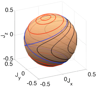
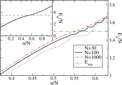
Figure 1: (color online). Left: Mean-field phase space of a BEC in a double-well potential given by the discrete Gross-Pitaevskii equation (3), for $u=5$. Self-trapping modes (red) coexist with Rabi-like oscillations (black). The two regions are separated by the separatrix (blue). There are two elliptic fixed points associated with self-trapped solutions. Right: The rescaled energy spectra $E_{n}/N$ of the BH Hamiltonian for various particle numbers $N$, and constant control parameter $u=5$. The separatrix energy $E_{\rm sep}$ is plotted as dash-double-dotted, horizontal, green line.

The dynamics generated by (3) is governed by the control parameter $u=UN/2k$ BES90 : For very small inter-particle interaction $u<1$, the BH system is in the Rabi regime, where the condensate oscillates between the two wells, i.e., the time-averaged population imbalance between them is zero (i.e., $\langle J_{z}\rangle_{t}=0$). In the other extreme of very strong interactions $u>N^{2}$, the system is in the self-trapped regime, where the condensate is persistently trapped in one of the wells, i.e., the average population imbalance between them is non-zero $\langle J_{z}\rangle_{t}\neq 0$.

For intermediate values of the control parameter $u\approx 1$ (Josephson regime) the phase space is divided by a separatrix located at the energy $E_{\rm sep}/N=k(u/2+1)$, and both the above dynamical modes coexist SLE85 ; BES90 ; ELS85 . In the left panel of Fig.1, we show the phase-space structure typical for this intermediate regime: For small initial particle imbalances (and phase difference $J_{x}\approx 0.5$) Rabi-like oscillations (black) rule the phase-space. Here, each trajectory corresponds to a situation where a fraction of the condensate oscillates between the two wells, while, on average, the bosons are equidistributed, i.e., $\langle J_{z}\rangle_{t}=0$. In this Rabi region of phase space and for a given energy, there exists exactly one trajectory.

In contrast, for sufficiently large initial population imbalance, one observes self-trapped trajectories (red). They encircle the stable fixed points located in the Northern (Southern) hemisphere and correspond to a persistent particle imbalance $J_{z}(t)>0$ ($J_{z}(t)<0$) for all times $t$. For a given energy in the self-trapped region of phase space, a pair of two solutions with inverse particle imbalance exists. The blue line denotes the separatrix.

This phase-space structure has a clear signature in the quantum energy spectrum of Hamiltonian (1) (cf. right panel of Fig. 1): Energy eigenstates below the separatrix energy $E_{\rm sep}$ are non-degenerate, since their mean-field counterpart are uniquely defined trajectories in the Rabi region. The appearance of two self-trapped trajectories of the same energy is quantum mechanically reflected in the fact that energy eigenstates above the separatrix energy are pairwise degenerate.

In the present paper, we concentrate on the Josephson regime of intermediate interactions ($u=5$), and large numbers of bosons in the double-well potential ($N\geq 30$). In the following, eigenstates whose mean-field counterpart are trajectories that show Rabi-like (self-trapping) behavior are called eigenstates in the Rabi (self-trapped) region of the spectrum.

We note that by construction (cf. Footnote 1) none of the eigenstates of (1) corresponds to a macroscopic superposition state. The creation of such states, their interaction with an electromagnetic field, and the resulting decoherence properties have been studied in detail by HM06 .

2.2 Scattering setup

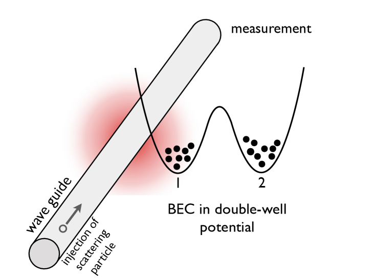
Figure 2: (color online). Scattering setup: The probe particle is injected into a waveguide that passes a condensate confined by a double-well potential. In the contact region between waveguide and site one of the double well, the probe particle and the BEC can exchange energy. The scattering quantities of the particle measured on exit from the waveguide carry detailed information on the state of the condensate.

We probe the double-well system by means of the scattering setup shown in Fig. 2 HHBCK10 : A probe particle with momentum $k$ moves in a waveguide that is placed in the proximity of say, site one of the double well. When the particle approaches the condensate, it interacts with the latter leading to an exchange of energy. On exit from the waveguide, typical scattering quantities of the probe particle, like e.g., its inelastic scattering probability, are measured. A possible experimental implementation of such scenario is provided by atom-chip setups, which allow for both, trapping of the BEC and (magnetic) guiding of the probe particle.

The waveguide in our scattering scheme is modeled by two semi-infinite tight-binding (TB) leads with hopping term $J$ and lattice spacing $a=1$. These two leads are coupled with strength $J_{0}$ to the central lead site $j=0$, which is closest to the condensate. Thus, $J_{0}\leq J$ determines the effective coupling strength between the leads and the projectile-target interaction region (i.e. for $J_{0}=0$ the latter is completely isolated) and hence controls the width of the scattering resonances. Consequently, the probe-particle Hamiltonian reads:

$$H_{\rm TB}=\Big{[}-J\sum_{j\neq-1,0}\hat{c}_{j}\hat{c}_{j+1}^{\dagger}-J_{0}\sum_{j=-1,0}\hat{c}_{j}\hat{c}_{j+1}^{\dagger}\Big{]}+{\rm h.c.}\,,$$ (4)

with $\hat{c}_{j}^{(\dagger)}$ the annihilation (creation) operators of the probe particle at site $j$ of the TB lead. The particle’s energy in the momentum eigenstate $|k_{m}\rangle$ is $\epsilon_{m}=-2J\cos(k_{m})$, with corresponding velocity $v_{m}=2J\sin(k_{m})$ Datta95 .

The probe-target interaction $H_{\rm int}$ is assumed to be of similar type (i.e. short range) as the bosonic inter-particle interaction in the condensate. Hence, it takes non-vanishing values only when the probe particle is located at the central lead site ($j=0$) which is closest to site one of the double well, and it is proportional to the number of bosons at this site:

$$H_{\rm int}=\alpha\cdot\hat{c}^{\dagger}_{0}\hat{c}_{0}\otimes\hat{n}_{1}\,,$$ (5)

$\alpha\!>\!0$ is a parameter that controls the strength of the probe-target interaction.

2.3 Scattering matrix

Given the total Hamiltonian

$$H_{\rm tot}=H_{\rm TB}\otimes{\hat{1}}+{\hat{1}}\otimes H_{\rm BH}+H_{\rm int}\,,$$ (6)

we can now define the scattering matrix of our problem: The condensate is initially prepared in an energy eigenstate $|E_{m}\rangle$, while the probe particle is injected with an energy $\epsilon_{m}$. Hence, asymptotically far from the interaction region, the total energy is ${\cal E}=E_{m}+\epsilon_{m}$. The open channels (modes) in the leads are then determined by energy conservation and the fact that the condensate’s final state is among the energy eigenstates $\{E_{n}\}$ of the BH Hamiltonian. Hence, the open modes are characterized by the kinetic energy $\epsilon_{n}={\cal E}-E_{n}$ of the outgoing probe particle. In other words, for a given total energy ${\cal E}$, the basis of our scattering problem is completely characterized by the Bose-Hubbard eigenstates, i.e. $\{|\epsilon_{n}\rangle\otimes|E_{n}\rangle\}\equiv\{|E_{n}\rangle\}$. The transmission block of the $S$-matrix then reads HHBCK10 :

$$[{\hat{S}}_{T}]({\cal E})=\sqrt{\hat{v}}\frac{i\,\gamma}{(1-\gamma)[{\cal E}-{\hat{H}}_{BH}]-\alpha{\hat{n}}_{1}+i\gamma{\hat{v}}}\sqrt{\hat{v}}\,,$$ (7)

where $\gamma\equiv(J_{0}/J)^{2}$, and ${\hat{v}}$ is the velocity operator. In the eigenbasis of the BH Hamiltonian, both ${\hat{H}}_{BH}$ and ${\hat{v}}$ become diagonal matrices i.e. $[H_{BH}]_{nm}=E_{n}\delta_{nm}$ and $v_{nm}=v_{n}\delta_{nm}$. In contrast, $Q_{nm}=\langle E_{n}|{\hat{n}}_{1}|E_{m}\rangle$ is, in general ($k\neq 0$), a non-diagonal matrix, what yields a non-diagonal $S_{T}$-matrix. This, in turn, corresponds to inelastic scattering and in that sense $\alpha$ controls the degree of inelasticity in the scattering process.

As known from scattering theory, the imaginary part of the $S$-matrix denominator determines the width of the resonances. Thus, in the present case, the coupling ratio $\gamma$ controls this width: For example, in the limit $\gamma\rightarrow 0$, the resonances become $\delta$-like, while they grow with increasing $\gamma$. For $\gamma=1$, Eq. (7) coincides with the $S$-matrix for inelastic electronic scattering in a 1D geometry derived in BC08 . Throughout the paper, we fix $\gamma=0.1$, corresponding to the intermediate regime of overlapping resonances.

3 Results

3.1 Interaction matrix $Q$

We start our analysis by a direct inspection of the probe-target interaction matrix $Q$ shown in the left panel of Fig. 3, for $N=100$ bosons. The value of the control parameter is $u=5$, what corresponds to intermediate inter-atomic interaction strengths in the BEC (see Fig. 1) and will be fixed throughout the paper. One immediately recognizes that $Q$ is a banded matrix that is divided into two halves by a “blurred” spot, located in the vicinity of level $n=56$. The behavior of the matrix elements in either region is quite different: Consider, for example, the diagonal elements $Q_{nn}=\langle E_{n}|{\hat{n}}_{1}|E_{n}\rangle$ that represent the expectation value of the boson number in well one, with respect to the energy eigenstate $|E_{n}\rangle$ (see full dots in the right panel of Fig. 3). Below the energy level $n=56$, $Q_{nn}$ takes the constant value $N/2$, what corresponds to equidistribution of the bosons among the two wells. Above this energy level, the expectation value of $\hat{n}_{1}$ begins to oscillate, e.g., in state $n=57$ only $31$ particles occupy site one, while in state $n=58$, the majority of $69$ bosons populates site one, and so on.

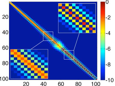
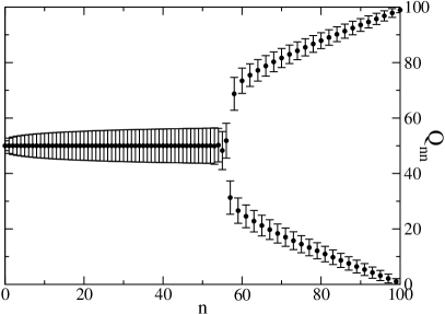
Figure 3: (color online). Left: Logarithmically color-coded snapshot of the interaction matrix $Q$, for $N=100$ particles and $u=5$. The insets show magnifications of the $Q$-matrix structure in the Rabi (left) and self-trapped (right) regime, respectively. Right: The expectation value $\langle E_{n}|\hat{n}_{1}|E_{n}\rangle=Q_{nn}$ of the bosonic number operator $\hat{n}_{1}$ versus the level index $n$, for identical parameters. The error bars denote the corresponding standard deviation $\sigma_{n}=\sqrt{\langle E_{n}|\hat{n}^{2}_{1}|E_{n}\rangle-\langle E_{n}|\hat{n}_{1}|E_{n}\rangle^{2}}$.

Besides the average value $Q_{nn}$, the corresponding standard deviation $\sigma_{n}=\sqrt{\langle E_{n}|\hat{n}^{2}_{1}|E_{n}\rangle-\langle E_{n}|\hat{n}_{1}|E_{n}\rangle^{2}}$ bears complementary information on the number fluctuations and is represented in Fig. 3 by the error bars. One clearly sees that $\sigma_{n}$ is largest in the vicinity of level $=56$ and takes its smallest values for the maximally localized states.

The observed behavior is a direct signature of the underlying mean-field dynamics of the BEC: We recall from the discussion in Sec. 2.1, that for $N=100$ bosons, the separatrix energy $E_{\rm sep}$ is located around energy level $E_{56}$ (see black solid curve of Fig. 1), i.e., around the same level at which the expectation value of $\hat{n}_{1}$ starts to oscillate. Hence, eigenstates $\{|E_{n}\rangle\}$ with expectation value $Q_{nn}=N/2$ correspond to those mean-field solutions that show, on average, vanishing particle imbalance $\langle J_{z}\rangle_{t}=0$, and thus belong to the Rabi region of the spectrum. The associated number fluctuations grow with increasing level index and take their maximum value close to the separatrix, where the mean-field oscillations in the $J_{z}$-direction of phase space are largest (see left panel of Fig. 1). On the other hand, states with index $n>56$ are alternatingly localized on either well and thus belong to the self-trapped region. Their fluctuations are reduced with increasing index $n$. In the mean-field phase space, increasing $n$ corresponds to trajectories that are closer and closer to the two elliptic fixed points, where the oscillations in any direction are zero.

Note also the checker-board structure in the interaction matrix $Q$ that is present in the self-trapped region and which implies that the interaction operator can solely induce transitions between self-trapped states located at the same well. In contrast, in the Rabi region, the odd off-diagonals are strongly populated, while the even off-diagonals vanish. This is due to the fact that the operator $\hat{n}_{1}$ does not commute with the parity operator ${\hat{P}}$, and can solely induce transitions between states with different parity (see Appendix A). Since energy eigenstates in the Rabi region of the spectrum have alternating parity, the even off-diagonal elements, which couple eigenstates with same parity, are zero. In both regimes, the value of the off-diagonal matrix elements decreases exponentially with the distance from the diagonal.

3.2 Participation number of $S_{T}$

How is the structure of $Q$, that encodes the properties of the BEC, reflected in the scattering signal? In the following, we will focus on the inelastic part of the scattering signal that, in contrast to the elastic part, accounts for all final configurations of the target, and thus bears much more detailed information. Consequently, we analyze the off-diagonal elements of the $S_{T}$-matrix.

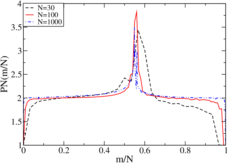
Figure 4: (color online). Participation number PN of the $S_{T}$-matrix versus the scaled level index $m/N$, for $u=5$, $\gamma=0.1$, $\alpha=1.0$, and various boson numbers $N$. The PN is averaged over the entire accessible energy axis ${\cal E}$. The peak around $m/N\approx 0.56$ reflects the separatrix (compare right panel of Fig. 1).

As a first step, we determine the number of final target configurations $|E_{n}\rangle$ for the BEC initially prepared in an eigenstate $|E_{m}\rangle$ ($m\neq n$). To this end, we define the participation number PN of each column of the $S_{T}$ -matrix:

$${\rm PN}(m)=\left[\frac{\sum_{n\neq m}|[S_{\rm T}]_{nm}|^{4}}{[\sum_{n\neq m}|[S_{\rm T}]_{nm}|^{2}]^{2}}\right]^{-1}\,.$$ (8)

Since the diagonal term $[S_{\rm T}]_{mm}$ is excluded from the summation, this quantity is meaningful only if the inelastic part of the scattering signal does not vanish, i.e. if $\alpha>0$. Then, PN reflects the number of outgoing channels that participate in the inelastic process, and hence takes values between one and $N$.

In Fig. 4, we plot the PN for intermediate probe-target interaction $\alpha=1$ and various boson numbers $N$, versus the scaled level index $m/N$. All curves approximately assume the value two, apart from the strong peak in the PN located around $m/N=0.56$. Recalling the above discussion, we relate its position to the separatrix energy $E_{\rm sep}$. Accordingly, for an initial preparation of the BEC in the self-trapped or Rabi region (i.e. $m/N\neq 0.56$), mainly two outgoing channels take part in the inelastic scattering, while this number is enhanced for initial preparations near the separatrix energy $E_{\rm sep}$.

The observed behavior is a consequence of the shape of the interaction matrix $Q$ (see Fig. 1) that can be understood from a semiclassical argument: In the self-trapped and Rabi regions, the mean-field counterpart of the interaction operator, $n(t)=|A_{1}(t)|^{2}$, oscillates with one unique frequency CSHKVC10 , what, upon quantization, yields one transition frequency, i.e., two off-diagonals in the $Q$-matrix. In contrast, close to the separatrix, the two distinct dynamical behaviors approach. Therefore, in a small energy window around $E_{\rm sep}$, several frequencies appear in the dynamics of $n(t)$, what leads to a larger number of off-diagonal elements in the interaction matrix $Q$.

3.3 Inelastic scattering cross section

Besides the participation number PN of the $S_{\rm T}$-matrix, an experimentally easily accessible quantity is the inelastic scattering cross section

$$\rho_{\rm in}^{m}({\cal E})=2\sum_{n\neq m}|[S_{T}]_{nm}|^{2}\,,$$ (9)

which denotes the probability to be scattered (forward and backward) from an incident channel $|\epsilon_{m}\rangle$ to any other channel $|\epsilon_{n}\rangle\neq|\epsilon_{m}\rangle$, or, equivalently, from a initially prepared condensate eigenstate $|E_{m}\rangle$ to a final eigenstate $|E_{n}\rangle$.

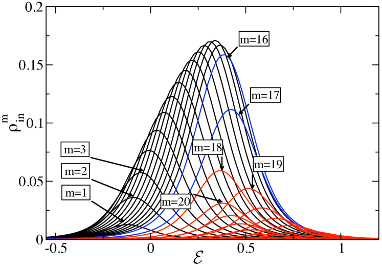
Figure 5: (color online). Inelastic cross section $\rho_{\rm in}^{n}$ versus the total energy ${\cal E}$, in units of the tunneling strength $k$. For better visibility we chose $N=30$ particles but otherwise same parameters as in Fig. 4. Some representative channels are labeled by their index $m$. The black (red) curves belong to preparations of the BEC in the Rabi (self-trapped) region of the spectrum, while the blue curves correspond to initial preparations in eigenstates with energies close to the separatrix energy.

In Fig. 5, we plot the inelastic cross section $\rho_{\rm in}^{m}({\cal E})$ as a function of the total energy ${\cal E}$, for all $m$. That is, each curve corresponds to an initial preparation of the BEC in a different energy eigenstate $|E_{m}\rangle$. We use the same parameters as in Fig. 4 and – for the sake of clarity – choose a smaller system with $N=30$ bosons. As the channel number increases from $m=1$ to $m=15$, the maximum of $\rho_{\rm in}^{m}({\cal E})$ – referred to in the following as the resonance position – monotonically shifts to larger energy values (solid black lines), until, around channels $m=16$ and $m=17$ (solid blue lines), the behavior changes. For channels $m\geq 18$ (red lines), the resonance position oscillates, i.e., for $\rho^{18}_{\rm in}$ it is located at ${\cal E}=0.36$, $\rho^{19}_{\rm in}$ becomes maximal at ${\cal E}=0.51$, while $\rho^{20}_{\rm in}$ takes its maximal value at ${\cal E}=0.38$, and so on.

This “splitting effect” is the most drastic consequence of the underlying mean-field dynamics. In Fig. 5, black curves correspond to the Rabi region, while red curves refer to self-trapping. Quite intuitively, one relates the oscillations of the resonance positions to the alternating mean occupation $Q_{nn}$ (see right panel in Fig. 3). In other words, for a pair of curves (like e.g. $\rho^{18}_{\rm in}$ and $\rho^{19}_{\rm in}$), the one with lower (higher) resonance position corresponds to a self-trapped state localized in well one (two).

This intuition is corroborated by a simplified expression for $\rho^{m}_{\rm in}({\cal E})$, that we derive from first-order perturbation theory with respect to the probe-target interaction strength $\alpha$ (see Appendix B), and which holds for the intermediate values of probe-target interaction $\alpha$ and coupling parameter $\gamma$ considered here:

$$\rho^{m}_{\rm in,Born}({\cal E}) \simeq 2{v}_{m}^{-1}\frac{\alpha^{2}{v}_{m}^{2}}{[(1-\gamma)({\cal E}-E_{m})-\alpha Q_{mm}]^{2}+\gamma^{2}{v}_{m}^{2}}$$ (10)

$$\times\left[\langle E_{m}|\hat{n}^{2}_{1}|E_{m}\rangle-\langle E_{m}|\hat{n}_{1}|E_{m}\rangle^{2}\right].$$

Neglecting for a moment the (weak) energy dependence of the velocity $v_{m}$, Eq. (10) takes a Lorentzian shape. Accordingly, the resonance positions are well approximated by $E_{n}+\alpha/(1-\gamma)Q_{nn}$. In the Rabi region, they thus experience a constant shift due to the approximately constant spacing of the BH energies $E_{n}$ (see right panel of Fig. 1). In contrast, self-trapped states are nearly pairwise degenerate and the spacing between adjacent pairs grows linearly. In this regime, the oscillation in the occupation number $Q_{nn}$ causes the splitting of the resonance positions.

We note that the only ingredients in (10) are the eigenenergy $E_{m}$ of the BH system, as well as the expectation value $Q_{mm}$ and variance $\sigma_{m}^{2}$ of the number counting operator $\hat{n}_{1}$ in the corresponding eigenstate $|E_{m}\rangle$. In comparison with the standard deviation $\sigma_{n}$ shown in Fig. 3, expression (10) reproduces quite well the overall trend of the inelastic cross section $\rho^{m}_{\rm in}({\cal E})$: In the Rabi as well as in the self-trapped region, $\rho^{m}_{\rm in}({\cal E})$ assumes its largest (smallest) values for initial target energies close to (far from) the separatrix energy $E_{\rm sep}$.

4 Conclusion

The properties of a BEC trapped in a double-well potential were analyzed via the inelastic, quantum mechanical scattering of a probe particle. Traces of the underlying mean-field phase space, like the appearance of self-trapped solutions, were unambiguously identified in various, experimentally accessible quantities. Based only on the expectation value and variance of the probe-target interaction operator, an analytical expression was derived that elucidates the main observations. Finally, the proposed scattering setup represents a non-destructive measurement of the condensate, what is in contrast to standard techniques, like time-of-flight imaging, that necessarily result in the destruction of the BEC.

Appendix A Parity in the Rabi region of the spectrum

In the Rabi region and for vanishing potential bias, the energy eigenstates $|E_{m}\rangle$ (with $E_{m}<E_{\rm sep}$) of the BH Hamiltonian have well-defined parity, i.e. ${\hat{P}}|E_{m}\rangle=\pm|E_{m}\rangle$, with ${\hat{P}}$ the parity operator that interchanges the particles between the two wells. We now show that the interaction operator $\hat{n}_{1}$ cannot induce transitions between energy eigenstates with same parity.

We first calculate the commutator $[{\hat{P}},\hat{n}_{1}]$. in the Fock basis $|n_{1},N-n_{1}\rangle\equiv|n_{1}\rangle$, where $n_{1}$ denotes the number of bosons in well one. In this basis, $\hat{P}|n_{1}\rangle=|N-n_{1}\rangle$, and we have

$$[{\hat{P}},{\hat{n}}_{1}]|n_{1}\rangle = (n_{1}{\hat{P}}-(N-n_{1}){\hat{P}})|n_{1}\rangle$$ (11)

$$= (2{\hat{n}}_{2}-N){\hat{P}}|n_{1}\rangle.$$

Assuming that the two energy eigenstates $|E_{m}\rangle$ and $|E_{n}\rangle$ ($m\neq n$) have same parity, we calculate the corresponding off-diagonal element of ${\hat{n}}_{1}$:

$$\langle E_{n}|{\hat{n}}_{1}|E_{m}\rangle = \langle E_{n}|{\hat{P}}{\hat{n}}_{1}{\hat{P}}|E_{m}\rangle$$ (12)

$$= \langle E_{n}|(2{\hat{n}}_{2}-N){\hat{P}}{\hat{P}}+{\hat{n}}_{1}{\hat{P}}{\hat{P}}|E_{m}\rangle$$

$$= \langle E_{n}|{\hat{n}}_{2}|E_{m}\rangle$$

$$= \langle E_{n}|N-\hat{n}_{1}|E_{m}\rangle=-\langle E_{n}|{\hat{n}}_{1}|E_{m}\rangle\,,$$

i.e. $\langle E_{n}|{\hat{n}}_{1}|E_{m}\rangle=0$.

Appendix B Perturbation theory

In this Appendix, we derive Eq. (10). The starting point of this calculation is the Born expansion of the $S_{T}$-matrix with respect to the perturbation parameter $\alpha$: We incorporate the diagonal of the $Q$-matrix,

$$\tilde{Q}_{nm}=\delta_{nm}Q_{nm}\,,$$ (13)

into the unperturbed Hamiltonian $H_{BH}$, and treat solely the non-diagonal part of the $Q$-matrix,

$$\bar{Q}=Q-\tilde{Q},$$ (14)

as the perturbation. Hence, we obtain as first-order Born approximation of (7) the following expression:

$$S_{T,\rm{Born}} = i\,{v}^{1/2}\frac{\gamma}{(1{-}\gamma)({\cal E}-H_{BH})-\alpha\tilde{Q}+i\gamma{v}}{v}^{1/2}$$ (15)

$$+ i\gamma\alpha\,\frac{{v}^{1/2}}{(1{-}\gamma)({\cal E}-H_{BH})-\alpha\tilde{Q}+i\gamma{v}}\bar{Q}$$

$$\times \frac{{v}^{1/2}}{(1{-}\gamma)({\cal E}-H_{BH})-\alpha\tilde{Q}+i\gamma{v}}\,.$$

Note that the first term in (15), termed $S_{D}$, is irrelevant for the inelastic cross section $\rho_{\rm in}$, since it is diagonal. We can further use the perturbative result (15), to obtain an analytical estimate for the inelastic cross section and the transmission probability. To this end, we rewrite (15) as:

$$S_{T,\rm{Born}} = S_{D}-i\kappa B$$ (16)

where $\kappa=\alpha/\gamma$ is the rescaled perturbation parameter and $B\equiv S_{D}{v}^{-\frac{1}{2}}\bar{Q}{v}^{-\frac{1}{2}}S_{D}$ is the rescaled perturbation operator. From Eqs. (9) and (16) one obtains the inelastic cross section:

$$\rho^{m}_{\rm in,\rm{Born}} = 2\kappa^{2}\left[\sum_{n}B_{mn}B_{nm}^{*}-B_{mm}B_{mm}^{*}\right]$$ (17)

$$= 2\kappa^{2}[\langle E_{m}|BB^{\dagger}|E_{m}\rangle-\langle E_{m}|B|E_{m}\rangle^{2}]\,.$$

It is interesting to note that, in leading order of $\kappa$, $\rho^{m}_{\rm in,Born}$ depends only on the variance of the perturbation operator $B$ in the eigenstate $|E_{m}\rangle$ of the Bose-Hubbard Hamiltonian. With the definition of $B$ and some basic algebra we obtain

$$\rho^{m}_{\rm in,Born}=$$

$$2\kappa^{2}{v}_{m}^{-1}\frac{\gamma^{2}{v}_{m}^{2}}{[(1-\gamma)({\cal E}-E_{m})-\alpha Q_{mm}]^{2}+\gamma^{2}{v}_{m}^{2}}$$ (18)

$$\times\sum_{k}\bar{Q}_{mk}\underbrace{{v}_{k}^{-1}\frac{\gamma^{2}{v}_{k}^{2}}{[(1-\gamma)({\cal E}-E_{k})-\alpha Q_{kk}]^{2}+\gamma^{2}{v}_{k}^{2}}}_{A}\bar{Q}_{km}\,.$$

In order to simplify the above formula, we assess the part $A$ in the last equation: We have numerically verified that for moderate values of $\alpha$ and $\gamma\leq 0.2$, each of the $A$-terms is equal or smaller than unity (apart from the ${v}_{k}^{-1}$ its a Lorentzian curve, i.e. we have to assure that ${v}_{k}^{-1}\leq 1$). The inelastic cross section is then given by:

$$\rho^{m}_{\rm in,Born} \geq 2{v}_{m}^{-1}\frac{\alpha^{2}{v}_{m}^{2}}{[(1-\gamma)({\cal E}-E_{m})-\alpha Q_{mm}]^{2}+\gamma^{2}{v}_{m}^{2}}$$ (19)

$$\times\left[\langle E_{m}|\hat{n}^{2}_{1}|E_{m}\rangle-\langle E_{m}|\hat{n}_{1}|E_{m}\rangle^{2}\right]\,.$$

References

- (1) M. Greiner, O. Mandel, T. Esslinger, et al., Nature 415, 6867 (2002)
- (2) J. Billy, V. Josse, Z. Zuo, et al., Nature 453, 891 (2008)
- (3) G. Roati, C. D’Errico, L. Fallani, et al., Nature 453, 895 (2008)
- (4) D. Hunger, S. Camerer, T. W. Hänsch, et al., Phys. Rev. Lett. 104, 143002 (2010)
- (5) B. Grüner, M. Jag, A. Stibor, et al., Phys. Rev. A 80, 063422 (2009)
- (6) D. Heine, M. Wilzbach, T. Raub, et al., Phys. Rev. A 79, 021804 (2009)
- (7) G. J. Milburn, J. Corney, E. Wright, et al., Phys. Rev. A 55, 4318 (1997)
- (8) M. Albiez, R. Gati, J. Folling, et al., Phys. Rev. Lett. 95, 010402 (2005)
- (9) M. Hiller, T. Kottos, A. Ossipov, Phys. Rev. A 73, 063625 (2006)
- (10) E. M. Graefe, H. J. Korsch, A. E. Niederle, Phys. Rev. Lett. 101, 150408 (2008)
- (11) D. Witthaut, F. Trimborn, S. Wimberger, Phys. Rev. Lett. 101, 200402 (2008)
- (12) K. Rapedius, H. J. Korsch, J. Phys. B 42, 044005 (2009)
- (13) B. Wu, Q. Niu, Phys. Rev. A 61, 023402 (2000)
- (14) K. Smith-Mannschot, M. Chuchem, M. Hiller, et al., Phys. Rev. Lett. 102, 230401 (2009)
- (15) D. Witthaut, E. M. Graefe, H. J. Korsch, Phys. Rev. A 73, 063609 (2006)
- (16) J. Javanainen, Phys. Rev. Lett. 57, 3164 (1986)
- (17) J. Estève, C. Gross, A. Weller, et al., Nature 455, 1216 (2008)
- (18) M. F. Riedel, P. Böhi, Y. Li, et al., Nature 464, 1170 (2010)
- (19) C. Gross, T. Zibold, E. Nicklas, et al., Nature 464, 1165 (2010)
- (20) A. Scott, P. Lomdahl, J. Eilbeck, Chem. Phys. Lett. 113, 29 (1985)
- (21) S. Hunn, M. Hiller, A. Buchleitner, et al., arXiv: 1010.2092 (2010)
- (22) D. Jaksch, C. Bruder, J. I. Cirac, et al., Phys. Rev. Lett. 81, 3108 (1998)
- (23) D. R. Dounas-Frazer, L. Carr, Phys. Rev. Lett. 99, 200402 (2007)
- (24) O. Morsch, M. Oberthaler, Rev. Mod. Phys. 78, 180 (2006)
- (25) L. Pitaevskii, S. Stringari, Bose-Einstein Condensation (Oxford Science Publications, Oxford, 2003)
- (26) L. Bernstein, J. C. Eilbeck, A. C. Scott, Nonlinearity 3, 293 (1990)
- (27) J. Eilbeck, P. Lomdahl, A. Scott, Physica 16D, 318 (1985)
- (28) S. Aubry, S. Flach, K. Kladko, et al., Phys. Rev. Lett. 76, 1607 (1996)
- (29) Y. P. Huang, M. G. Moore, Phys. Rev. A 73, 023606 (2006)
- (30) S. Datta, Electronic Transport in Mesoscopic Systems (Cambridge University Press, 1995)
- (31) Bandopadhyay, D. Cohen, Phys. Rev. B 77, 155438 (2008)
- (32) M. Chuchem, K. Smith-Mannschott, M. Hiller, et al., Phys. Rev. A 82, 053617 (2010)
- (33) D. Cohen, T. Kottos, Phys. Rev. E 63, 036203 (2001)
- (34) M. Hiller, T. Kottos, T. Geisel, Phys. Rev. A 79, 023621 (2009)