New molecular candidates: $X(1910)$, $X(2200)$, and $X(2350)$

Abstract

Assuming the newly observed resonant structures $X(1910)$, $X(2200)$, and $X(2350)$ as $\omega\omega$, $\omega\phi$, and $\phi\phi$ molecular states respectively, we compute their mass values in the framework of QCD sum rules. The numerical results are $1.97\pm 0.17~{}\mbox{GeV}$ for $\omega\omega$ state, $2.07\pm 0.21~{}\mbox{GeV}$ for $\omega\phi$ state, and $2.18\pm 0.29~{}\mbox{GeV}$ for $\phi\phi$ state, which coincide with the experimental values of $X(1910)$, $X(2200)$, and $X(2350)$, respectively. This supports the statement that $X(1910)$, $X(2200)$, and $X(2350)$ could be $\omega\omega$, $\omega\phi$, and $\phi\phi$ molecular candidates respectively.

I Introduction

Very recently, Belle Collaboration reported observations of new resonant structures at $M(\omega\omega)\sim 1.91~{}\mbox{GeV}$, $M(\omega\phi)\sim 2.2~{}\mbox{GeV}$, and $M(\phi\phi)\sim 2.35~{}\mbox{GeV}$ in $\gamma\gamma\rightarrow X\rightarrow\omega\omega$, $\omega\phi$, and $\phi\phi$ respectively X . For convenience, these resonances are called $X(1910)$, $X(2200)$, and $X(2350)$ here. Since they all decay into two light vector mesons, it is natural to suppose them to be molecular bound states composed of two light mesons. In theory, the molecular concept was put forward long ago Voloshin and it was predicted that molecular states have a rich spectroscopy in Ref. Glashow . The possible deuteron-like two-meson bound states were studied in Ref. NAT . Although molecular states have not been confirmed in experiment, there already have had some candidates for them. For instance, $Y(4260)$ could be a $\chi_{c}\rho^{0}$ Y4260-Liu or an $\omega\chi_{c1}$ state Y4260-Yuan ; $Z^{+}(4430)$ could be a $D^{*}\bar{D}_{1}$ state theory-Z4430n ; theory-Z4430 ; $Y(3930)$ is proposed to be a $D^{*}\bar{D}^{*}$ theory-Y3930 ; Liu ; 3930-Ping ; $Y(4140)$ is interpreted as a $D_{s}^{*}\bar{D}_{s}^{*}$ Liu ; theory-Y4140 ; $X(4350)$ could be a $D_{s}^{*}D_{s}^{0*}$ X4350-Zhang ; X4350-Ma ; $Y(4274)$ could be a $D_{s}D_{s0}(2317)$ Y4274-Liu . For more molecular candidates, one can also see some other Refs., e.g. reviews ; reviews1 . If molecular states can be completely confirmed by experiment, QCD will be further testified and then one will comprehend the QCD low-energy behaviors more deeply. Therefore, it is interesting to study whether the newly observed $X$ states could be molecular states.

In the real world, quarks are confined inside hadrons and the strong interaction dynamics of hadronic systems is governed by nonperturbative QCD effect completely. Many questions concerning dynamics of the quarks and gluons at large distances remain unanswered or, at most, understood only at a qualitative level. It is a great challenge to extract hadronic information quantitatively from the rather simple Lagrangian of QCD. Fortunately, one can apply the QCD sum rule method svzsum (for reviews see overview1 ; overview2 ; overview3 ; overview4 and references therein), which is a nonperturbative formulation firmly based on QCD basic theory and has been successfully employed to some light four-quark states HXChen ; HXChen1 ; HXChen2 ; Zs ; ALZhang ; ZGWang ; Nielsen . In Ref. qqqq , the authors have studied the tetraquark state $qq\bar{q}\bar{q}$ by constructing and analyzing the sum rule composed of a diquark-antidiquark current with the quantum number $J^{P}=0^{+}$ and found masses of the tetraquark state $qq\bar{q}\bar{q}$ appear in the region of $0.6\sim 1~{}\mbox{GeV}$, which are much lower than the mass of $X(1910)$. Thereby, it may not likely to be a $qq\bar{q}\bar{q}$ tetraquark state for $X(1910)$. In Ref. qqss , the authors have studied the tetraquark $ud\bar{s}\bar{s}$ of $J^{P}=0^{+}$ in the QCD sum rule and the mass of the tetraquark turns out to be around $1.5~{}\mbox{GeV}$, which is much lower than the mass of $X(2200)$. Thus, it may not likely to be a tetraquark $ud\bar{s}\bar{s}$ for $X(2200)$. In Ref. ssss , the authors have predicted the mass of $ss\bar{s}\bar{s}$ tetraquark state of $J^{P}=0^{+}$ to be about $2.2~{}\mbox{GeV}$ in the relativistic quark model, which is slightly lower than the mass of $X(2350)$. Just from the slight mass difference, one may not judge that $X(2350)$ is unlikely to be a $ss\bar{s}\bar{s}$ tetraquark state. However, one could at least see that the result does not exclude other possible interpretations such as molecular picture for $X(2350)$. Therefore, we intend to obtain mass information of $\omega\omega$, $\omega\phi$, and $\phi\phi$ bound states from QCD sum rules, and investigate whether $X(1910)$, $X(2200)$, and $X(2350)$ could be new molecular candidates.

The rest of the paper is organized as three parts. We discuss QCD sum rules for molecular states in Sec. II, with the similar procedure as our previous works Zhang . The numerical analysis is made in Sec. III, and masses of $\omega\omega$, $\omega\phi$, and $\phi\phi$ states are extracted out. The Sec. IV includes a brief summary and outlook.

II QCD sum rules for $\omega\omega$, $\omega\phi$, and $\phi\phi$ molecular states

The starting point of the QCD sum rule is to construct the interpolating current properly and then write down the correlator. In full QCD, the interpolating current for light vector meson can be found e.g. in Ref. reinders . One can construct the molecular state current from meson-meson type of fields. Meanwhile, note that Belle Collaboration have indicated that there are substantial $0^{+}$ components in all three modes ($\gamma\gamma\rightarrow X\rightarrow\omega\omega$, $\omega\phi$, and $\phi\phi$). Thus, following forms of currents with $J^{P}=0^{+}$ are constructed for $\omega\omega$, $\omega\phi$, and $\phi\phi$

$$j_{\omega\omega} = (\bar{q}_{c}\gamma^{\mu}q_{c})(\bar{q}_{c^{\prime}}\gamma_{\mu}q_{c^{\prime}}),$$ (1)

$$j_{\omega\phi} = (\bar{q}_{c}\gamma^{\mu}q_{c})(\bar{s}_{c^{\prime}}\gamma_{\mu}s_{c^{\prime}}),$$ (2)

$$j_{\phi\phi} = (\bar{s}_{c}\gamma^{\mu}s_{c})(\bar{s}_{c^{\prime}}\gamma_{\mu}s_{c^{\prime}}),$$ (3)

where $q$ denotes light quarks $u$ and $d$, with $c$ and $c^{\prime}$ are color indices. One should note that meson molecules in the real world are long objects in which the quark pairs are far away from each other. The currents in this work and in most of the QCD sum rule works are local and the four field operators here act at the same space-time point. It is a limitation inherent in the QCD sum rule disposal of the hadrons since the bound states are not point particles in a rigorous manner. The two-point correlator is defined as $\Pi(q^{2})=i\int d^{4}x\mbox{e}^{iq.x}\langle 0|T[j(x)j^{+}(0)]|0\rangle$. In phenomenology, the correlator can be expressed as

$$\Pi(q^{2})=\frac{\lambda_{H}^{2}}{M_{H}^{2}-q^{2}}+\frac{1}{\pi}\int_{s_{0}}^{\infty}ds\frac{\mbox{Im}\Pi^{\mbox{phen}}(s)}{s-q^{2}}+\mbox{subtractions},$$ (4)

where $M_{H}$ is the mass of the hadronic resonance, and $\lambda_{H}$ gives the coupling of the current to the hadron $\langle 0|j|H\rangle=\lambda_{H}$. In the operator product expansion (OPE) side, the correlator can be written as

$$\Pi(q^{2})=\int_{s_{min}}^{\infty}ds\frac{\rho^{\mbox{OPE}}(s)}{s-q^{2}}+\Pi^{\mbox{cond}}(q^{2}),$$ (5)

where the spectral density is $\rho^{\mbox{OPE}}(s)=\frac{1}{\pi}\mbox{Im}\Pi^{\mbox{OPE}}(s)$, with the integration limit $s_{min}\approx 0$ for $\omega\omega$ state, $s_{min}=(2m_{s})^{2}$ for $\omega\phi$ state, and $s_{min}=(4m_{s})^{2}$ for $\phi\phi$ state. After equating the two sides, assuming quark-hadron duality, and making a Borel transform, the sum rule can be written as

$$\lambda_{H}^{2}e^{-M_{H}^{2}/M^{2}} = \int_{s_{min}}^{s_{0}}ds\rho^{\mbox{OPE}}e^{-s/M^{2}}+\hat{B}\Pi^{\mbox{cond}},$$ (6)

where $M^{2}$ indicates the Borel parameter. To eliminate the hadronic coupling constant $\lambda_{H}$, one reckons the ratio of derivative of the sum rule to itself, and then yields

$$M_{H}^{2} = \Bigg{\{}\int_{s_{min}}^{s_{0}}ds\rho^{\mbox{OPE}}se^{-\frac{s}{M^{2}}}+\frac{d(\hat{B}\Pi^{\mbox{cond}})}{d(-\frac{1}{M^{2}})}\Bigg{\}}\Bigg{/}\Bigg{\{}\int_{s_{min}}^{s_{0}}ds\rho^{\mbox{OPE}}e^{-\frac{s}{M^{2}}}+\hat{B}\Pi^{\mbox{cond}}\Bigg{\}}.$$ (7)

For the OPE calculations, we work at the leading order in $\alpha_{s}$ and consider condensates up to dimension ten, utilizing the light-quark propagator in the coordinate-space

$$S_{ab}(x) = \frac{i\delta_{ab}}{2\pi^{2}x^{4}}\hbox to0.0pt{/\hss}x-\frac{m_{q}\delta_{ab}}{4\pi^{2}x^{2}}-\frac{i}{32\pi^{2}x^{2}}t^{A}_{ab}gG^{A}_{\mu\nu}(\hbox to0.0pt{/\hss}x\sigma^{\mu\nu}+\sigma^{\mu\nu}\hbox to0.0pt{/\hss}x)-\frac{\delta_{ab}}{12}\langle\bar{q}q\rangle+\frac{i\delta_{ab}}{48}m_{q}\langle\bar{q}q\rangle\hbox to0.0pt{/\hss}x$$

$${}-\frac{x^{2}\delta_{ab}}{3\cdot 2^{6}}\langle g\bar{q}\sigma\cdot Gq\rangle+\frac{ix^{2}\delta_{ab}}{2^{7}\cdot 3^{2}}m_{q}\langle g\bar{q}\sigma\cdot Gq\rangle\hbox to0.0pt{/\hss}x-\frac{x^{4}\delta_{ab}}{2^{10}\cdot 3^{3}}\langle\bar{q}q\rangle\langle g^{2}G^{2}\rangle.$$

The $s$ quark is dealt as a light one and the diagrams are considered up to the order $m_{s}$. For some minor multi-gluon condensate contributions, one could omit them as the usual treatment. Concretely, spectral densities can be written as

$$\rho^{\mbox{pert}}(s)=\frac{1}{5\cdot 2^{12}\pi^{6}}s^{4},~{}~{}~{}\rho^{\langle\bar{q}q\rangle^{2}}(s)=\frac{\langle\bar{q}q\rangle^{2}}{2^{3}\pi^{2}}s,~{}~{}~{}\rho^{\langle\bar{q}q\rangle\langle g\bar{q}\sigma\cdot Gq\rangle}(s)=-\frac{\langle\bar{q}q\rangle\langle g\bar{q}\sigma\cdot Gq\rangle}{2^{3}\pi^{2}},$$

$$\hat{B}\Pi^{\mbox{cond}}=\frac{\langle g\bar{q}\sigma\cdot Gq\rangle\langle g\bar{q}\sigma\cdot Gq\rangle}{2^{6}\pi^{2}}+\frac{\langle\bar{q}q\rangle^{2}\langle g^{2}G^{2}\rangle}{3^{2}\cdot 2^{5}\pi^{2}},$$

for $\omega\omega$ state,

$$\rho^{\mbox{pert}}(s)=\frac{1}{5\cdot 2^{12}\pi^{6}}s^{4},~{}~{}~{}\rho^{\langle\bar{s}s\rangle^{2}}(s)=\frac{\langle\bar{s}s\rangle^{2}}{2^{4}\pi^{2}}s,~{}~{}~{}\rho^{\langle\bar{q}q\rangle^{2}}(s)=\frac{\langle\bar{q}q\rangle^{2}}{2^{4}\pi^{2}}s,~{}~{}~{}\rho^{\langle g\bar{s}\sigma\cdot Gs\rangle}(s)=\frac{\langle g\bar{s}\sigma\cdot Gs\rangle}{2^{7}\pi^{4}}m_{s}s,$$

$$\rho^{\langle\bar{s}s\rangle\langle g^{2}G^{2}\rangle}(s)=-\frac{\langle\bar{s}s\rangle\langle g^{2}G^{2}\rangle}{3\cdot 2^{8}\pi^{4}}m_{s},~{}~{}~{}\rho^{\langle\bar{s}s\rangle\langle g\bar{s}\sigma\cdot Gs\rangle}(s)=-\frac{\langle\bar{s}s\rangle\langle g\bar{s}\sigma\cdot Gs\rangle}{2^{4}\pi^{2}},~{}~{}~{}\rho^{\langle\bar{q}q\rangle\langle g\bar{q}\sigma\cdot Gq\rangle}(s)=-\frac{\langle\bar{q}q\rangle\langle g\bar{q}\sigma\cdot Gq\rangle}{2^{4}\pi^{2}}$$

$$\hat{B}\Pi^{\mbox{cond}}=-\frac{m_{s}}{2}\langle\bar{q}q\rangle^{2}\langle\bar{s}s\rangle+\frac{\langle g\bar{s}\sigma\cdot Gs\rangle^{2}}{2^{7}\pi^{2}}+\frac{\langle g\bar{q}\sigma\cdot Gq\rangle^{2}}{2^{7}\pi^{2}}+\frac{\langle\bar{s}s\rangle^{2}\langle g^{2}G^{2}\rangle}{3^{2}\cdot 2^{6}\pi^{2}}+\frac{\langle\bar{q}q\rangle^{2}\langle g^{2}G^{2}\rangle}{3^{2}\cdot 2^{6}\pi^{2}},$$

for $\omega\phi$ state, and

$$\rho^{\mbox{pert}}(s)=\frac{1}{5\cdot 2^{12}\pi^{6}}s^{4},~{}~{}~{}\rho^{\langle\bar{s}s\rangle^{2}}(s)=\frac{\langle\bar{s}s\rangle^{2}}{2^{3}\pi^{2}}s,~{}~{}~{}\rho^{\langle g\bar{s}\sigma\cdot Gs\rangle}(s)=\frac{\langle g\bar{s}\sigma\cdot Gs\rangle}{2^{6}\pi^{4}}m_{s}s,$$

$$\rho^{\langle\bar{s}s\rangle\langle g^{2}G^{2}\rangle}(s)=-\frac{\langle\bar{s}s\rangle\langle g^{2}G^{2}\rangle}{3\cdot 2^{7}\pi^{4}}m_{s},~{}~{}~{}\rho^{\langle\bar{s}s\rangle\langle g\bar{s}\sigma\cdot Gs\rangle}(s)=-\frac{\langle\bar{s}s\rangle\langle g\bar{s}\sigma\cdot Gs\rangle}{2^{3}\pi^{2}},$$

$$\hat{B}\Pi^{\mbox{cond}}=-m_{s}\langle\bar{s}s\rangle^{3}+\frac{\langle g\bar{s}\sigma\cdot Gs\rangle\langle g\bar{s}\sigma\cdot Gs\rangle}{2^{6}\pi^{2}}+\frac{\langle\bar{s}s\rangle^{2}\langle g^{2}G^{2}\rangle}{3^{2}\cdot 2^{5}\pi^{2}},$$

for $\phi\phi$ state.

III Numerical analysis and discussions

The sum rule (7) is numerically analyzed in this section. The input values are taken as $m_{s}=0.10^{+0.03}_{-0.02}~{}\mbox{GeV}$ PDG , $\langle\bar{q}q\rangle=-(0.23\pm 0.03)^{3}~{}\mbox{GeV}^{3}$, $\langle g\bar{q}\sigma\cdot Gq\rangle=m_{0}^{2}~{}\langle\bar{q}q\rangle$, $\langle\bar{s}s\rangle=-(0.8\pm 0.1)\times(0.23\pm 0.03)^{3}~{}\mbox{GeV}^{3}$, $\langle g\bar{s}\sigma\cdot Gs\rangle=m_{0}^{2}~{}\langle\bar{s}s\rangle$, $m_{0}^{2}=0.8\pm 0.1~{}\mbox{GeV}^{2}$, and $\langle g^{2}G^{2}\rangle=0.88~{}\mbox{GeV}^{4}$ overview2 . Complying with the criterion of sum rule analysis, the threshold $\sqrt{s_{0}}$ and Borel parameter $M^{2}$ are varied to find the optimal stability window. In the standard QCD sum rule approach, one can analyse the convergence in the OPE side and the pole contribution dominance in the phenomenological side to determine the conventional Borel window: on one hand, the lower constraint for $M^{2}$ is obtained by the consideration that the perturbative contribution should be larger than condensate contributions; on the other hand, the upper bound for $M^{2}$ is obtained by the restriction that the pole contribution should be larger than the continuum state contributions. Meanwhile, the threshold $\sqrt{s_{0}}$ is not arbitrary but characterizes the beginning of continuum states. For many hadrons, the first excitation of studied state defines the size of $\sqrt{s_{0}}$, and the difference between $\sqrt{s_{0}}$ and the mass $M_{H}$ of studied state is around $0.5~{}\mbox{GeV}$. Concretely, the value of $\sqrt{s_{0}}$ is fixed by these steps: 1) taking a value of $\sqrt{s_{0}}$; 2) fixing the corresponding Borel parameters $M^{2}$ according to two rules (OPE convergence and pole dominance); 3) extracting the mass from the sum rule in the work window fixed in the first and second steps; 4) checking that whether the $\sqrt{s_{0}}$ chosen in the first step is acceptable using the empirical relation that the difference between $\sqrt{s_{0}}$ and $M_{H}$ is around $0.5~{}\mbox{GeV}$; 5) if the $\sqrt{s_{0}}$ chosen in the first step is not acceptable, return to the first step, vary $\sqrt{s_{0}}$ and go on. Taking $\omega\omega$ as an example, we choose $\sqrt{s_{0}}=2.4~{}\mbox{GeV}$ and finally arrive at $M_{H}=1.97~{}\mbox{GeV}$. One could check that $\sqrt{s_{0}}=2.4~{}\mbox{GeV}$ is acceptable with the empirical relation that the difference between $\sqrt{s_{0}}$ and $M_{H}$ is around $0.5~{}\mbox{GeV}$. Thus, we choose the central value of $\sqrt{s_{0}}=2.4~{}\mbox{GeV}$ for $\omega\omega$ state.

Here, we would make some particular discussions on the choice of Borel windows. It has been shown in detail in some Refs, such as qqqq and Matheus , that it is not possible to find an conventional Borel window for some light scalar tetraquarks. The problem is that the four-quark condensate is very large, making the standard OPE convergence to happen only at very large values of $M^{2}$. In fact, it has appeared the same problem in this work. Taking the $\omega\omega$ as an example, the comparison between pole and continuum contributions from sum rule (6) for $\omega\omega$ state for $\sqrt{s_{0}}=2.4~{}\mbox{GeV}$ is shown in the left panel of FIG. 1, and its OPE convergence by comparing the perturbative with other condensate contributions is shown in the right panel. Even if we choose some uncritical convergence criteria, e.g. the perturbative contribution should be at least bigger than each condensate contribution, there is no standard OPE convergence up to $M^{2}\geq 1.8~{}\mbox{GeV}^{2}$. The consequence is that it is unable to find the conventional Borel window where both the OPE converges well (i.e. the perturbative contribution bigger than each condensate contribution) and the pole dominates over the continuum (the latter one happens at $M^{2}\leq 1.3~{}\mbox{GeV}^{2}$). Under such a circumstance, one could try several possible ways to solve the problem. I) One could release the criterion of pole dominating over continuum and take some high values of Borel parameter $M^{2}$. Thus, OPE series can converge well. Graphically from the Borel curve, one can see that there is a very stable plateau. Some authors have virtually adopted this way to deal with the above problem. However, there occurs some other problem. Although there is very good OPE convergence and a flat plateau for the Borel curve, contributions from continuum states are dominating. As one knows, the phenomenological side of the sum rule can be expressed as $\Pi(q^{2})=\frac{\lambda_{H}^{2}}{M_{H}^{2}-q^{2}}+\frac{1}{\pi}\int_{s_{0}}^{\infty}ds\frac{\mbox{Im}\Pi^{\mbox{phen}}(s)}{s-q^{2}}$ due to the “single-pole+continuum states” hypothesis. From the criterion of pole dominating over continuum, one can obtain the maximal value of the Borel parameter $M^{2}$ satisfying the “single-pole+continuum states” model. Exceeding this value of $M^{2}$, the single-pole dominance condition will be spoiled. Thereby, the Borel parameter $M^{2}$ must not be chosen too large to warrant pole dominance. II) One could push the threshold parameter $\sqrt{s_{0}}$ to a very large value, and the maximum value of $M^{2}$ will be enhanced with the increasing of $\sqrt{s_{0}}$. Thus, one may find the Borel window satisfying both the perturbative bigger than condensate contributions and the pole bigger than continuum contributions. However, the threshold parameter $\sqrt{s_{0}}$ is not arbitrary but characterizes the beginning of the continuum states. With too large values of $\sqrt{s_{0}}$, contributions from high resonance states and continuum states may be included in the pole contribution. Hence, the QCD sum rule may not work normally. III) One could warrant the pole dominance firstly and try releasing the strict convergence criterion of perturbative contribution larger than each condensate contribution in some case. In the present work, we have dealt with the problem in this way. It is worth to note that the treatment is not arbitrary but there is some definite condition. For example, we consider the ratio of perturbative contribution to the “total OPE contribution” (the sum of perturbative and other condensate contributions calculated) but not the ratio of perturbative contribution to each condensate contribution. Not too bad, there are two main condensate contributions with different signs (four-quark condensate and two-quark multiply mixed condensate) and they could cancel with each other to some extent, which brings that the ratio of perturbative contribution to the “total OPE contribution” is bigger than $60\%$ at $M^{2}\geq 0.8~{}\mbox{GeV}^{2}$ for $\omega\omega$ for $\sqrt{s_{0}}=2.4~{}\mbox{GeV}$. In addition, we calculate and find that the ratio of perturbative contribution to the “total OPE contribution” does not change much including some high dimension condensate contributions. In this sense, we could say that the OPE converges in the region while satisfying pole dominance. Although it may not be good OPE convergence in comparison with the conventional case, one could find a comparatively reasonable work window. Note that the treatment should not be arbitrarily transplanted to any case. One could take the Ref. Matheus as an example. From its FIG. 4, one can see that for $f_{0}$ all condensate contributions in the region $0.4\leq M^{2}\leq 0.7~{}\mbox{GeV}^{2}$ are larger than the perturbative contribution. That means one could not even find a region that the perturbative dominates in the “total OPE” allowed by the upper bound. In a word, to deal with the problem on choosing the conventional Borel window in QCD sum rules, which have similarly appeared in some other multiquark states, we warrant the pole dominance preferably and release the strict convergence criterion to a weak one that perturbative dominates in “total OPE contribution”, so that the convergence of OPE is still under control while satisfying pole dominance. Although it may not be so good OPE convergence as the conventional case, one could find a comparatively reasonable work window and extract the hadronic information of studied states reliably. Thus, we choose the minimum value of $M^{2}$ to be $0.8~{}\mbox{GeV}^{2}$ and the maximum $M^{2}$ to be $1.3~{}\mbox{GeV}^{2}$ for $\omega\omega$ state for $\sqrt{s_{0}}=2.4~{}\mbox{GeV}$. Similarly, the maximum value of $M^{2}$ is taken as $1.2~{}\mbox{GeV}^{2}$ for $\sqrt{s_{0}}=2.3~{}\mbox{GeV}$; for $\sqrt{s_{0}}=2.5~{}\mbox{GeV}$, the maximum $M^{2}$ is taken as $1.4~{}\mbox{GeV}^{2}$. The dependence on $M^{2}$ for the mass of $\omega\omega$ state from sum rule (7) is shown in FIG. 2, and we arrive at $1.97\pm 0.07~{}\mbox{GeV}$ for $\omega\omega$ state. Considering the uncertainty rooting in the variation of quark masses and condensates, we gain $1.97\pm 0.07\pm 0.10~{}\mbox{GeV}$ (the first error reflects the uncertainty due to variation of $\sqrt{s_{0}}$ and $M^{2}$, and the second error resulted from the variation of QCD parameters) or $1.97\pm 0.17~{}\mbox{GeV}$ for $\omega\omega$ state.

The comparison between pole and continuum contributions from sum rule (6) for $\omega\phi$ state for $\sqrt{s_{0}}=2.6~{}\mbox{GeV}$ is shown in the left panel of FIG. 3, and its OPE convergence by comparing the perturbative with other condensate contributions is shown in the right panel. There has the same problem for $\omega\phi$ as the above case for $\omega\omega$, and we treat it similarly. For $\omega\phi$ state, the ratio of perturbative to the “total OPE contribution” at $M^{2}=1.1~{}\mbox{GeV}^{2}$ for $\sqrt{s_{0}}=2.6~{}\mbox{GeV}$ is around $67\%$ and increases with the $M^{2}$. Furthermore, the relative pole contribution is approximate to $54\%$ at $M^{2}=1.5~{}\mbox{GeV}^{2}$ and descends with the $M^{2}$. Thus, the range of $M^{2}$ is taken as $M^{2}=1.1\sim 1.5~{}\mbox{GeV}^{2}$ for $\sqrt{s_{0}}=2.6~{}\mbox{GeV}$. Similarly, the proper range of $M^{2}$ is obtained as $1.1\sim 1.4~{}\mbox{GeV}^{2}$ for $\sqrt{s_{0}}=2.5~{}\mbox{GeV}$, and the range of $M^{2}$ is $1.1\sim 1.6~{}\mbox{GeV}^{2}$ for $\sqrt{s_{0}}=2.7~{}\mbox{GeV}$. The mass of $\omega\phi$ state as a function of $M^{2}$ from sum rule (7) is shown in FIG. 4, and we obtain $2.07\pm 0.13~{}\mbox{GeV}$ for $\omega\phi$. Varying input values of quark masses and condensates, we attain $2.07\pm 0.13\pm 0.08~{}\mbox{GeV}$ (the first error reflects the uncertainty due to variation of $\sqrt{s_{0}}$ and $M^{2}$, and the second error resulted from the variation of QCD parameters) or $2.07\pm 0.21~{}\mbox{GeV}$ for $\omega\phi$ state.

For $\phi\phi$ state, the comparison between pole and continuum contributions from sum rule (6) for $\sqrt{s_{0}}=2.7~{}\mbox{GeV}$ is shown as an example in the left panel of FIG. 5, and its OPE convergence by comparing the perturbative with other condensate contributions is shown in the right panel. A bit difference for the case of $\phi\phi$ is that the perturbative contribution can be bigger than the second most important condensate $\langle\bar{s}s\rangle^{2}$ at $M^{2}\geq 1.1~{}\mbox{GeV}^{2}$. Meanwhile, the pole contribution can dominate in the total contribution while $M^{2}\leq 1.6~{}\mbox{GeV}^{2}$. Thus, it is possible to find a region where both the OPE can converge well (the perturbative contribution bigger than each condensate contribution) and the pole dominates over the continuum. Thus, the range of $M^{2}$ for $\phi\phi$ state is taken as $M^{2}=1.1\sim 1.6~{}\mbox{GeV}^{2}$ for $\sqrt{s_{0}}=2.7~{}\mbox{GeV}$. Via the similar analyzing process, the proper range of $M^{2}$ is obtained as $1.1\sim 1.7~{}\mbox{GeV}^{2}$ for $\sqrt{s_{0}}=2.8~{}\mbox{GeV}$, and the range of $M^{2}$ is $1.1\sim 1.8~{}\mbox{GeV}^{2}$ for $\sqrt{s_{0}}=2.9~{}\mbox{GeV}$. In the chosen region, the corresponding Borel curve to determine the mass of $\phi\phi$ state is shown in FIG. 6, and we extract the mass value $2.18\pm 0.20~{}\mbox{GeV}$ for $\phi\phi$ state. Subsequently, we vary the quark masses as well as condensates and arrive at $2.18\pm 0.20\pm 0.09~{}\mbox{GeV}$ (the first error reflects the uncertainty due to variation of $\sqrt{s_{0}}$ and $M^{2}$, and the second error resulted from the variation of QCD parameters) or $2.18\pm 0.29~{}\mbox{GeV}$ in a concise form.

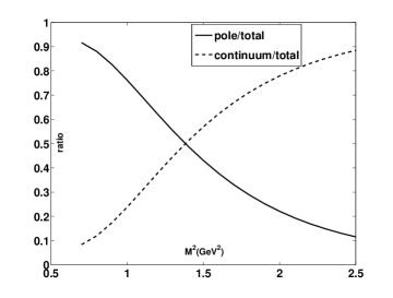
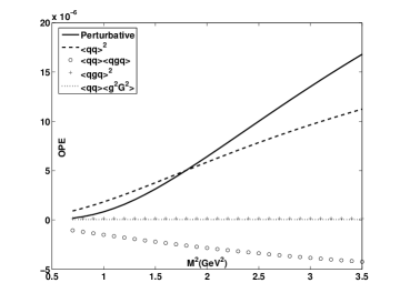
Figure 1: In the left panel, the solid line shows the relative pole contribution (the pole contribution divided by the total, pole plus continuum contribution) and the dashed line shows the relative continuum contribution from sum rule (6) for $\sqrt{s_{0}}=2.4~{}\mbox{GeV}$ for $\omega\omega$ state. The OPE convergence is shown by comparing the perturbative with other condensate contributions from sum rule (6) for $\sqrt{s_{0}}=2.4~{}\mbox{GeV}$ for $\omega\omega$ state in the right panel.

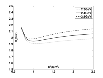
Figure 2: The mass of $\omega\omega$ state as a function of $M^{2}$ from sum rule (7) is shown. The continuum thresholds are taken as $\sqrt{s_{0}}=2.3\sim 2.5~{}\mbox{GeV}$. For $\sqrt{s_{0}}=2.3~{}\mbox{GeV}$, the range of $M^{2}$ is $0.8\sim 1.2~{}\mbox{GeV}^{2}$; for $\sqrt{s_{0}}=2.4~{}\mbox{GeV}$, the range of $M^{2}$ is $0.8\sim 1.3~{}\mbox{GeV}^{2}$; for $\sqrt{s_{0}}=2.5~{}\mbox{GeV}$, the range of $M^{2}$ is $0.8\sim 1.4~{}\mbox{GeV}^{2}$.

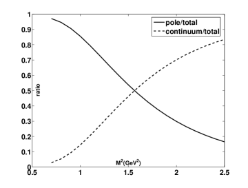
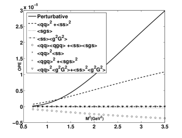
Figure 3: In the left panel, the solid line shows the relative pole contribution (the pole contribution divided by the total, pole plus continuum contribution) and the dashed line shows the relative continuum contribution from sum rule (6) for $\sqrt{s_{0}}=2.6~{}\mbox{GeV}$ for $\omega\phi$ state. The OPE convergence is shown by comparing the perturbative with other condensate contributions from sum rule (6) for $\sqrt{s_{0}}=2.6~{}\mbox{GeV}$ for $\omega\phi$ state in the right panel.

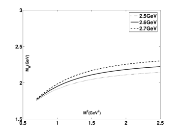
Figure 4: The mass of $\omega\phi$ state as a function of $M^{2}$ from sum rule (7) is shown in the right panel. The continuum thresholds are taken as $\sqrt{s_{0}}=2.5\sim 2.7~{}\mbox{GeV}$. For $\sqrt{s_{0}}=2.5~{}\mbox{GeV}$, the range of $M^{2}$ is $1.1\sim 1.4~{}\mbox{GeV}^{2}$; for $\sqrt{s_{0}}=2.6~{}\mbox{GeV}$, the range of $M^{2}$ is $1.1\sim 1.5~{}\mbox{GeV}^{2}$; for $\sqrt{s_{0}}=2.7~{}\mbox{GeV}$, the range of $M^{2}$ is $1.1\sim 1.6~{}\mbox{GeV}^{2}$.

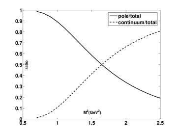
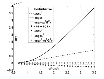
Figure 5: In the left panel, the solid line shows the relative pole contribution (the pole contribution divided by the total, pole plus continuum contribution) and the dashed line shows the relative continuum contribution from sum rule (6) for $\sqrt{s_{0}}=2.7~{}\mbox{GeV}$ for $\phi\phi$ state. The OPE convergence is shown by comparing the perturbative with other condensate contributions from sum rule (6) for $\sqrt{s_{0}}=2.7~{}\mbox{GeV}$ for $\phi\phi$ state in the right panel.

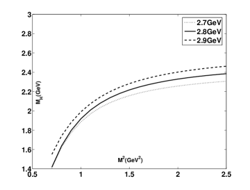
Figure 6: The mass of $\phi\phi$ state as a function of $M^{2}$ from sum rule (7) is shown. The continuum thresholds are taken as $\sqrt{s_{0}}=2.7\sim 2.9~{}\mbox{GeV}$. For $\sqrt{s_{0}}=2.7~{}\mbox{GeV}$, the range of $M^{2}$ is $1.1\sim 1.6~{}\mbox{GeV}^{2}$; for $\sqrt{s_{0}}=2.8~{}\mbox{GeV}$, the range of $M^{2}$ is $1.1\sim 1.7~{}\mbox{GeV}^{2}$; for $\sqrt{s_{0}}=2.9~{}\mbox{GeV}$, the range of $M^{2}$ is $1.1\sim 1.8~{}\mbox{GeV}^{2}$.

IV Summary and outlook

In $\gamma\gamma\rightarrow X\rightarrow\omega\omega$, $\omega\phi$, and $\phi\phi$, Belle Collaboration observed three new resonant structures at $M(\omega\omega)\sim 1.91~{}\mbox{GeV}$, $M(\omega\phi)\sim 2.2~{}\mbox{GeV}$, and $M(\phi\phi)\sim 2.35~{}\mbox{GeV}$. Assuming these newly observed resonances as molecular states, we have employed the QCD sum rule method to calculate their masses, taking into account contributions of operators up to dimension ten in the OPE. Our final numerical results are $1.97\pm 0.17~{}\mbox{GeV}$ for $\omega\omega$ state, $2.07\pm 0.21~{}\mbox{GeV}$ for $\omega\phi$ state, and $2.18\pm 0.29~{}\mbox{GeV}$ for $\phi\phi$ state, which are in agreement with the experimental values of $X(1910)$, $X(2200)$, and $X(2350)$ respectively. This supports the statement that $X(1910)$, $X(2200)$, and $X(2350)$ could be $\omega\omega$, $\omega\phi$, and $\phi\phi$ molecular states respectively. However, one should note that there are still some differences between our central values and experimental values. At present, we have merely considered $\omega\omega$, $\omega\phi$, and $\phi\phi$ molecular states with $J^{P}=0^{+}$. Belle Collaboration indicated that while there are substantial spin-$0$ components in all three modes (namely $\gamma\gamma\rightarrow X\rightarrow\omega\omega$, $\omega\phi$, and $\phi\phi$), there are also spin-$2$ components near threshold. The differences between our central values and experimental data are probably caused by that we have not considered the spin-$2$ components for $\omega\omega$, $\omega\phi$, and $\phi\phi$ state here, which implies that the theoretical predictions might be improved by including $J=2$ components for the future. In addition, one needs to take into account other dynamical analysis to identify the nature structures of these $X$ States for further work.

References

• (1) Z. Q. Liu et al., (Belle Collaboration), Phys. Rev. Lett. 108, 232001 (2012).
• (2) M. B. Voloshin and L. B. Okun, JETP Lett. 23, 333 (1976).
• (3) A. D. Rujula, H. Georgi, and S. L. Glashow, Phys. Rev. Lett. 38, 317 (1977).
• (4) N. A. Törnqvist, Z. Phys. C 61, 525 (1994).
• (5) X. Liu, X. Q. Zeng, and X. Q. Li, Phys. Rev. D 72, 054023 (2005).
• (6) C. Z. Yuan, P. Wang, and X. H. Mo, Phys. Lett. B 634, 399 (2006).
• (7) J. L. Rosner, Phys. Rev. D 76, 114002 (2007).
• (8) C. Meng and K. T. Chao, arXiv:0708.4222; X.  Liu, Y. R. Liu, W. Z. Deng, and S. L. Zhu, Phys. Rev. D 77, 034003 (2008); X. Liu, Y. R. Liu, W. Z. Deng, and S. L. Zhu, Phys. Rev. D 77, 094015 (2008).
• (9) X. Liu, Z. G. Luo, Y. R. Liu, and S. L. Zhu, Eur. Phys. J. C 61, 411 (2009).
• (10) X. Liu and S. L. Zhu, Phys. Rev. D 80, 017502 (2009).
• (11) Y. C. Yang and J. L. Ping, Phys. Rev. D 81, 114025 (2010).
• (12) N. Mahajan, Phys. Lett. B 679, 228 (2009); T. Branz, T. Gutsche, and V. E. Lyubovitskij, Phys. Rev. D 80, 054019 (2009); G. J. Ding, Eur. Phys. J. C 64, 297 (2009).
• (13) J. R. Zhang and M. Q. Huang, Commun. Theor. Phys. 54, 1075 (2010).
• (14) Y. L. Ma, Phys. Rev. D 82, 015013 (2010).
• (15) X. Liu, Z. G. Luo, and S. L. Zhu, Phys. Lett. B 699, 341 (2011).
• (16) M. Nielsen, F. S. Navarra, and S. H. Lee, Phys. Rep. 497, 41 (2010).
• (17) C. Y. Wong, Phys. Rev. C 69, 055202 (2004); N. A. Törnqvist, Phys. Lett. B 590, 209 (2004); F. E. Close and P. R. Page, Phys. Lett. B 578, 119 (2004); E. S. Swanson, Phys. Lett. B 588, 189 (2004).
• (18) M. A. Shifman, A. I. Vainshtein, and V. I. Zakharov, Nucl. Phys. B147, 385 (1979); B147, 448 (1979); V. A. Novikov, M. A. Shifman, A. I. Vainshtein, and V. I. Zakharov, Fortschr. Phys. 32, 585 (1984).
• (19) B. L. Ioffe, in The Spin Structure of The Nucleon, edited by B. Frois, V. W. Hughes, and N. de Groot (World Scientific, Singapore, 1997).
• (20) S. Narison, QCD Spectral Sum Rules (World Scientific, Singapore, 1989).
• (21) P. Colangelo and A. Khodjamirian, in At the Frontier of Particle Physics: Handbook of QCD, edited by M. Shifman, Boris Ioffe Festschrift Vol. 3 (World Scientific, Singapore, 2001), pp. 1495-1576; A. Khodjamirian, Continuous Advances in QCD 2002/ARKADYFEST.
• (22) M. Neubert, Phys. Rev. D 45, 2451 (1992); M. Neubert, Phys. Rep. 245, 259 (1994).
• (23) H. X. Chen, X. Liu, A. Hosaka, and S. L. Zhu, Phys. Rev. D 78, 034012 (2008).
• (24) H. X. Chen, A. Hosaka, and S. L. Zhu, Phys. Rev. D 76, 094025 (2007); Phys. Rev. D 78, 054017 (2008); Phys. Rev. D 78, 117502 (2008).
• (25) H. X. Chen, A. Hosaka, H. Toki, and S. L. Zhu, Phys. Rev. D 81, 114034 (2010).
• (26) J. R. Zhang, L. F. Gan, and M. Q. Huang, Phys. Rev. D 85, 116007 (2012).
• (27) A. L. Zhang, T. Huang, and T. G. Steele, Phys. Rev. D 76, 036004 (2007).
• (28) Z. G. Wang and W. M. Yang, Eur. Phys. J. C 42, 89 (2005); Z. G. Wang, Nucl. Phys. A 791, 106 (2007).
• (29) T. V. Brito, F. S. Navarra, M. Nielsen, and M. E. Bracco, Phys. Lett. B 608, 69 (2005).
• (30) H. X. Chen, A. Hosaka, and S. L. Zhu, Phys. Lett. B 650, 369 (2007).
• (31) H. X. Chen, A. Hosaka, and S. L. Zhu, Phys. Rev. D 74, 054001 (2006).
• (32) D. Ebert, R. N. Faustov, and V. O. Galkin, Eur. Phys. J. C 60, 273 (2009).
• (33) J. R. Zhang and M. Q. Huang, Phys. Rev. D 80, 056004 (2009); J. Phys. G: Nucl. Part. Phys. 37, 025005 (2010); JHEP 1011, 057 (2010); Phys. Rev. D 83, 036005 (2011); J. R. Zhang, M. Zhong, and M. Q. Huang, Phys. Lett. B 704, 312 (2011).
• (34) L. J. Reinders, H. R. Rubinstein, and S. Yazaki, Phys. Rep. 127, 1 (1985).
• (35) K. Nakamura et al., (Particle Data Group), J. Phys. G 37, 075021 (2010).
• (36) R. D. Matheus, F. S. Navarra, M. Nielsen, and R. Rodrigues da Silva, Phys. Rev. D 76, 056005 (2007).