Transformation between $\tau$ and TCB for Deep Space Missions under IAU Resolutions ^∗

Abstract

For tracking a spacecraft and doing radio science, the transformation between the proper time $\tau$ given by a clock carried on board a spacecraft and the barycentric coordinate time (TCB) is investigated under IAU resolutions. In order to show more clearly physical pictures and improve computational efficiency, an analytic approach is adopted. After numerical checks, it shows this method is qualified for a Mars orbiter during one year, especially being good at describing the influence from perturbing bodies. Further analyses demonstrate that there are two main effects in the transformation: the gravitational field of the Sun and the velocity of the spacecraft in the barycentric coordinate reference system (BCRS). The whole contribution of them is at the level of a few sub-seconds.

1 Introduction

Last a few decades see the enormous improvements of the accuracy of measurements and the unprecedented progress in techniques. It makes the general relativity (GR) become an inevitable part of the data processing in the high-precision observations. Thus, the first order post-Newtonian (1PN) general relativistic theory of astronomical reference frames based on [Brumberg & Kopejkin (1989)] and [Damour et al. (1991)], was adopted by General Assembly of the International Astronomical Union (IAU) in 2000 ([Soffel et al. (2003)]). Likewise, GR plays an important role for deep space missions in navigation and scientific experiments.

For example, the radio link connecting a spacecraft and a ground station has been a sensitive and useful tool for probing the interior structure of a body in the Solar System. Some signals from these intriguing but subtle effects might entangle with those due to the curved spacetime. This work is then motivated as the first step to construct an applicable and consistent relativistic framework that will be able to separate the planetary information from GR “bias”. On the other hand, the radio link in the interplanetary space could test theories of gravity. In 2003, the Cassini spacecraft had confirmed GR to an accuracy of $10^{-5}$ by Doppler tracking in the spacecraft solar conjunction ([Bertotti, Iess & Tortora (2003)]). This result has not only verified GR but also ruled out some theories which unsatisfied the corresponding condition. Deep space missions might also be opening a new window to some new physical laws at the scale of the solar system with the challenge of unexplained anomalies ([Anderson et al. (1998), Anderson et al.(2008)]). This is the reason why a complete data reduction framework should be established robustly in the first place to interpret the observation data.

A general scheme for data reduction based on a relativistic framework is represented as follows. Starting from a Lagrangian based theory of gravity, the metric of the Solar System can be obtained by the post-Newtonian approximation ([Chandrasekhar (1965)]). A global reference system covering the region of the whole spacetime is introduced to describe the orbital motions of the bodies in the Solar System. Some local reference systems are also introduced and each of them covers the nearby region of a body to define the multiple moments of the body and describe the motions of its massless satellites. However, most of current data reductions, including lunar laser ranging, are conducted in the global frame. Thus, it involves the coordinate transformation between the global frame and the local one. This transformation has been intensively studied by [Brumberg & Kopejkin (1989)], [Damour et al. (1991)], [Klioner & Soffel (2000)],[Kopeikin & Vlasov (2004)] and [Xie & Kopeikin (2010)]. Within this relativistic framework, the motions of spacecrafts, celestial bodies, light rays (photons) and observers in the Solar System would be adequately represented in different reference frames. The task is to make a relativistic model for a specific kind of observations with some physical or conventional quantities.

In the above process, different time scales exist within the relativistic framework by a contrast to Newton’s idea of absolute spacetime. A clock on board a spacecraft gives the proper time $\tau$, which is a physical time. To deal with the propagation of the signals emitted by a spacecraft in the Solar System, the Barycentric Celestial Reference System (BCRS) is usually used. It has a coordinate time component, called the barycentric coordinate time (TCB). Therefore $\tau$ needs to be connected with TCB at first for the whole radio link. This is one of our motivation in the research work. In general, a numerical method or an analytic one could be adopted for discussing this transformation. Although the numerical method is more competent for computing, inverting and predicting astronomical events and phenomena, it is not enough to provide some physical information. With a practical case in hand, the method can not distinguish the leading terms, the secular terms accumulated with time and the negligible terms from the numerical results. Besides, the presence of hundreds of terms with using higher approximation (for example, from 1PN to 2PN) makes these problems more complicated. However, the analytic method is extraordinarily good at these. Especially, the computational process by the analytic method is more time-saving and efficient. In the gauge-invariant point of view, some spurious coordinate-dependent effects can be removed by the analytic method. Thus a more efficient and unambiguous method should be found for providing to the above advantages. This is the another motivation of this paper.

To sum up, as a first step, employed an analytic method, this work mainly focuses on the transformation between the proper time $\tau$ on the spacecraft and TCB under IAU resolutions. It shows there exists the difference of two time system between on the spacecraft and on the global system. This transformation will be applied for connecting the emitted signal with the light propagation. It will also be applied by tracking, telemetry and control in ground stations.

We summarize some conventions and notations used in the paper. The metric signature is $(-,+,+,+)$; $G$ is the Newtonian constant of gravitation; $c$ is the velocity of the light and $\epsilon\equiv 1/c$; The capital subscripts $A$, $B$, $C$ $\ldots$ refer to the gravitating bodies in the solar system; The subscripts $T$ and $s$ denote respectively quantities related to the target body and the spacecraft; The Latin indices $i,j,k\ldots$ denote three-dimensional space components; The symmetric and trace-free (STF) part of a tensor $I^{ij}$ is denoted by $I^{<ij>}$; We also use multi-index notations such as $I^{<L>}\equiv I^{<i_{1}i_{2}\ldots i_{l}>}$. Section 2 is devoted to an analytic expression for the transformation between $\tau$ and TCB under IAU resolutions. Considering a Mars mission, the comparison between the numerical method and our analytic one is described in Section 3. Then, in Section 4, some results are derived with our analytic method. Finally, the conclusion and discussion are outlined in Section 5.

2 Model and analytic expression

In BCRS, the metric tensor under IAU resolutions ([Soffel et al. (2003)]) reads as

$$g_{00} = -1+\epsilon^{2}2w-\epsilon^{4}2w^{2}+\mathcal{O}(5),$$ (1)

$$g_{0i} = -\epsilon^{3}4w^{i}+\mathcal{O}(5),$$ (2)

$$g_{ij} = \delta_{ij}(1+\epsilon^{2}2w)+\mathcal{O}(4),$$ (3)

where $w$ and $w^{i}$ are respectively scalar and vector potentials. And $\mathcal{O}(n)$ means of the order $\epsilon^{n}$. Then, the transformation between the proper time of a spacecraft $\tau_{s}$ and TCB ($t$) can be done by integrating the following equations

$$\frac{\mathrm{d}\tau_{s}}{dt} = 1-\epsilon^{2}\bigg{(}w+\frac{1}{2}v^{2}_{s}\bigg{)}+\epsilon^{4}\bigg{(}\frac{1}{2}w^{2}+4w^{k}v^{k}_{s}-\frac{3}{2}wv^{2}_{s}-\frac{1}{8}v^{4}_{s}\bigg{)}+\mathcal{O}(5).$$ (4)

In principle, $w$ and $w^{i}$ should be expressed as the local multipole moments. But, if we only consider $N$-point masses with spins, Eq. (4) yields

$$\frac{\mathrm{d}\tau_{s}}{dt} = 1-\epsilon^{2}\bigg{(}\sum_{A}\frac{Gm_{A}}{r_{sA}}+\frac{1}{2}v^{2}_{s}\bigg{)}$$ (5)

$$-\epsilon^{4}\bigg{[}\frac{1}{8}v^{4}_{s}-\frac{1}{2}\sum_{A}\frac{G^{2}m^{2}_{A}}{r^{2}_{sA}}+2\sum_{A}\frac{Gm_{A}}{r_{sA}}v^{2}_{A}+\frac{3}{2}\sum_{A}\frac{Gm_{A}}{r_{sA}}v^{2}_{s}$$

$$-\frac{1}{2}\sum_{A}\frac{Gm_{A}}{r^{3}_{sA}}(r^{k}_{sA}v^{k}_{A})^{2}-4\sum_{A}\frac{Gm_{A}}{r_{sA}}v^{k}_{s}v^{k}_{A}$$

$$-4\sum_{A}\frac{G}{r^{3}_{sA}}\varepsilon^{k}_{~{}ij}S^{i}_{A}r^{j}_{sA}v^{k}_{s}-\frac{1}{2}\sum_{A}\sum_{B\neq A}\frac{G^{2}m_{A}m_{B}}{r_{sA}r_{sB}}$$

$$-\sum_{A}\sum_{B\neq A}\frac{G^{2}m_{A}m_{B}}{r_{sA}r_{AB}}+\frac{1}{2}\sum_{A}\sum_{B\neq A}\frac{G^{2}m_{A}m_{B}}{r_{sA}r^{3}_{AB}}r^{k}_{sA}r^{k}_{AB}\bigg{]},$$

where 1PN masses are obtained by using the method of two effective time-dependent masses of the $A$-th body

$$\tilde{\mu}_{A} = m_{A}\bigg{\{}1+\epsilon^{2}\bigg{[}-\sum_{B\neq A}\frac{Gm_{B}}{r_{AB}}+\frac{3}{2}v^{2}_{A}\bigg{]}\bigg{\}}+\mathcal{O}(4),$$ (6)

$$\mu_{A} = m_{A}\bigg{\{}1+\epsilon^{2}\bigg{[}-\sum_{B\neq A}\frac{Gm_{B}}{r_{AB}}+\frac{1}{2}v^{2}_{A}\bigg{]}\bigg{\}}+\mathcal{O}(4),$$ (7)

based on [Blanchet, Faye & Ponsot (1998)]. And $r_{sA}=|\mbox{\boldmath$x$\unboldmath}_{s}-\mbox{\boldmath$x$\unboldmath}_{A}|$, $r_{AB}=|\mbox{\boldmath$x$\unboldmath}_{A}-\mbox{\boldmath$x$\unboldmath}_{B}|$. $\mbox{\boldmath$x$\unboldmath}_{s}$ and $\mbox{\boldmath$x$\unboldmath}_{A}$ respectively denote positions of the spacecraft and the $A$-th body in BCRS. $\mbox{\boldmath$v$\unboldmath}_{s}$ and $\mbox{\boldmath$v$\unboldmath}_{A}$ respectively denote velocities of the spacecraft and the $A$-th body in BCRS. $\varepsilon^{k}_{~{}ij}$ is the fully antisymmetric Levi-Civita symbol and $S^{i}_{A}$ is the spin of the $A$-th body. In this paper, we mainly consider the effects for terms of Eq. (5) in the order of $\epsilon^{2}$ on the transformation. Namely,

$$\frac{\mathrm{d}\tau_{s}}{dt} = 1-\epsilon^{2}\bigg{(}\sum_{A}\frac{Gm_{A}}{r_{sA}}+\frac{1}{2}v^{2}_{s}\bigg{)}+\mathcal{O}(\epsilon^{4}).$$ (8)

The first term in the order of $\epsilon^{2}$ is a dynamical term which is contributed from $N$-body’s gravitational fields. The second term in Eq. (8) at the order $\epsilon^{2}$ is a kinematic term which comes from the velocity of the spacecraft. For the dynamical term, we split it into two parts:

$$\sum_{A}\frac{Gm_{A}}{r_{sA}} = \sum_{A\neq T}\frac{Gm_{A}}{r_{sA}}+\frac{Gm_{T}}{r_{sT}},$$ (9)

where the first one comes from the contribution of perturbing bodies and the second one is caused by the target body for the deep space mission. There exists a small quantity $q\equiv r_{sT}/r_{AT}$, which describes the distance between the spacecraft and the target body divided by the distance between the target body and the perturbing body. For the perturbing terms, they can be expanded by $q^{k}$ ($k=0,1,2,\ldots$) and show

$$\sum_{A\neq T}\frac{Gm_{A}}{r_{sA}} = \sum_{A\neq T}\frac{Gm_{A}}{|\mbox{\boldmath$x$\unboldmath}_{A}-\mbox{\boldmath$x$\unboldmath}_{T}-(\mbox{\boldmath$x$\unboldmath}_{s}-\mbox{\boldmath$x$\unboldmath}_{T})|}$$ (10)

$$= \sum_{A\neq T}\sum_{k=0}^{l}\frac{(2k-1)!!}{k!}\frac{Gm_{A}}{r^{2k+1}_{AT}}r^{<K>}_{AT}r^{<K>}_{sT}+\mathcal{O}(\sum_{k=l+1}^{\infty})$$

$$= \underbrace{\underbrace{\underbrace{\sum_{A\neq T}\frac{Gm_{A}}{r_{AT}}}_{l=0}+\sum_{A\neq T}\frac{Gm_{A}}{r^{3}_{AT}}r^{k}_{AT}r^{k}_{sT}}_{l=1}+\frac{3}{2}\sum_{A\neq T}\frac{Gm_{A}}{r^{5}_{AT}}r^{<i}_{AT}r^{j>}_{AT}r^{<i}_{sT}r^{j>}_{sT}}_{l=2}+\mathcal{O}(\sum_{k=3}^{\infty}).$$

For the dynamical term of perturbations, the above analytic expression will be converged with the increase of index $k$. In our research, we mainly focus on the first three terms, which correspond to $l=2$. In the next section, we will prove the difference between the analytic method and the numerical one for the perturbations is negligible for current accuracy.

Our task is to give the analytic expression of Eq. (8) at the order of $\epsilon^{2}$. The positions and velocities of the bodies and the spacecraft in the solar system are obtained by treating them as $N$ two-body problems. For example, the motions of eight planets with respect to the Sun are considered as 8 two-body problems and the motion of the spacecraft with respect to its target body is also considered as a two-body problem. For planet $A$, its position $\mbox{\boldmath$r$\unboldmath}^{Heli}_{A}$ and velocity $\mbox{\boldmath$v$\unboldmath}^{Heli}_{A}$ are expressed with the orbital elements in the heliocentric coordinate system as two-body problem ([Murray & Dermott (2000)]). Those elements are changing with time, such as $a_{A}=a_{A0}+\dot{a}_{A}T_{eph}$, $e_{A}=e_{A0}+\dot{e}_{A}T_{eph}$ and so on, based on Table 1 in Technical Report of JPL ([Standish]), where $T_{eph}$ is the number of centuries past J2000.0. With the positions and velocities of eight planets in the heliocentric coordinate system obtained, the position and velocity of the solar system barycenter (SSB) in the heliocentric coordinate system are then respectively obtained by $\sum_{A}m_{A}\mbox{\boldmath$r$\unboldmath}^{Heli}_{A}/\sum_{A}m_{A}$ and $\sum_{A}m_{A}\mbox{\boldmath$v$\unboldmath}^{Heli}_{A}/\sum_{A}m_{A}$. Using the positions of the planets and SSB in the heliocentric coordinate system, we could obtain the positions and the velocities of the Sun, Mercury, Venus, the Earth-Moon Barycenter (EMB), Mars, Jupiter, Saturn, Uranus and Neptune in BCRS. For $r^{i}_{sT}$, we solve it from the two-body problem in the equatorial reference system of the target body ([Murray & Dermott (2000)]). Furthermore, we rotate vector $r^{i}_{sT}$ from the equatorial reference system to the International Celestial Reference System (ICRS) based on the procedures recommended by the IAU/IAG Working Group on cartographic coordinates and rotational elements ([Archinal et al.(2011)]). The propose of above rotations is to deal with the coupling terms with vectors calculated in different reference systems.

For the kinematic term of Eq. (8), we only focus on the two-body interactions and omit others bodies’ perturbations

$$v^{2}_{s} = (\mbox{\boldmath$V$\unboldmath}_{s}+\mbox{\boldmath$v$\unboldmath}_{T})\cdot(\mbox{\boldmath$V$\unboldmath}_{s}+\mbox{\boldmath$v$\unboldmath}_{T})+\mathcal{O}(\epsilon^{2},\mathrm{others})$$ (11)

$$= v^{2}_{T}+V^{2}_{s}+2\mbox{\boldmath$v$\unboldmath}_{T}\cdot\mbox{\boldmath$V$\unboldmath}_{s}+\mathcal{O}(\epsilon^{2},\mathrm{others})$$

$$= Gm_{\odot}\bigg{(}\frac{2}{r_{T\odot}}-\frac{1}{a_{T}}\bigg{)}+Gm_{T}\bigg{(}\frac{2}{r_{sT}}-\frac{1}{a_{s}}\bigg{)}+2\mbox{\boldmath$v$\unboldmath}_{T}\cdot\mbox{\boldmath$V$\unboldmath}_{s}+\ldots,$$

where subscripts “$s$”, “$\odot$” and “$T$” denote the terms related to the spacecraft, the Sun and the target body, respectively. And $\mbox{\boldmath$v$\unboldmath}_{T}$ denotes the velocity vector of the target body in BCRS, and $\mbox{\boldmath$V$\unboldmath}_{s}$ denotes the velocity vector of the spacecraft in the target body’s local reference system. For $\mbox{\boldmath$v$\unboldmath}_{T}\cdot\mbox{\boldmath$V$\unboldmath}_{s}$ in Eq. (11), we must put the two vectors in the same coordinate system such as BCRS. $\mbox{\boldmath$V$\unboldmath}_{s}$ can be written as $(V_{s},0,0)^{T}$ in (U, N, W) triad where U points to the tangent direction of the orbit. Furthermore, we rotate this vector to the (S, T, W) triad where S points to the radial direction, then to the equatorial plane of the target body and finally to BCRS. Such a transformation is conducted by $R_{3}(-90^{\circ}-\alpha_{T})R_{1}(\delta_{T}-90^{\circ})R_{3}(-\Omega)R_{1}(-i)R_{3}(-\omega-f)R_{3}(\theta)(V_{s},0,0)^{T}$, where $\alpha_{T}$ and $\delta_{T}$ are ICRF equatorial coordinates at epoch J2000.0 for the north pole of one target body; $\Omega$ denotes longitude of ascending node for the spacecraft; $i$ denotes inclination of orbit for the spacecraft; $\omega$ denotes longitude of periastron for the spacecraft; $f$ is the true anomaly and $\theta$ is the angle between the tangent direction and transverse direction of the orbit, and $\cos\theta=(1+e\cos f)/\sqrt{1+2e\cos f+e^{2}}$.

Then, the analytic relation between $\tau_{s}$ and $t$ is

$$\tau_{s}-t = -\epsilon^{2}\int\bigg{[}\sum_{A\neq T}\frac{Gm_{A}}{r_{AT}}+\sum_{A\neq T}\frac{Gm_{A}}{r^{3}_{AT}}r^{k}_{AT}r^{k}_{sT}+\frac{3}{2}\sum_{A\neq T}\frac{Gm_{A}}{r^{5}_{AT}}r^{<i}_{AT}r^{j>}_{AT}r^{<i}_{sT}r^{j>}_{sT}+\frac{Gm_{T}}{r_{sT}}\bigg{]}\mathrm{d}t$$ (12)

$$-\epsilon^{2}\int\bigg{[}Gm_{\odot}\bigg{(}\frac{1}{r_{T\odot}}-\frac{1}{2a_{T}}\bigg{)}+Gm_{T}\bigg{(}\frac{1}{r_{sT}}-\frac{1}{2a_{s}}\bigg{)}+\mbox{\boldmath$v$\unboldmath}_{T}\cdot\mbox{\boldmath$V$\unboldmath}_{s}\bigg{]}\mathrm{d}t$$

$$+\mathcal{O}(\epsilon^{2},l\geq 3,\mathrm{others}),$$

where the positions and the velocities of $N$-body and the spacecraft can easily obtained just by two-body problem solutions. Compared to the numerical method, this analytic approach is more efficient in computation. In next section, we will prove it is qualified by the numerical check.

3 Numerical check

In this section, we will check our analytic result by comparison with the numerical results under a Mars mission. We simulate a spacecraft has a very large elliptical orbit around Mars from Nov. 01, 2012 to Nov. 01, 2013. Its orbital inclination to the Mars equator is about $5^{\circ}$. The apoapsis altitude is $80,000$km and the periapsis altitude is $800$km, with period of about 3 days.

Figure 1: Left: 3D orbital motion of the spacecraft for probing Mars (in kilometers). Middle: The distance $R$ (in kilometers) between Mars’ center and the spacecraft versus the time (in days). Right: The velocity of the spacecraft $V_{s}$ (in kilometers per second) with respect to the center of mass of Mars versus the time (in days).

In the simulation, the positions and the velocities of the planets and the Sun are read from the ephemeris DE405. For the initial conditions of the spacecraft, we calculate them from its orbital elements in the Mars equatorial reference frame and transfer them into the ICRS for numerical integration. For one year mission, the precession and nutation are negligible in the rotation elements of Mars for this transformation. So we only consider the fixed term for the north pole of Mars, namely, $\alpha_{0}=317^{\circ}.68143$ and $\delta_{0}=52^{\circ}.88650$ (see [Archinal et al.(2011)]). The integrator we use is the RKF7(8) ([Fehlberg (1968)]) with fixed step-size $30$ minutes.

In Fig. 1, our numerical results for the spacecraft are displayed. The left one shows its 3D orbit and we can see a large ellipse. The middle one shows the change of its distance from Mars with time. We can see the max value and the min value of $R$. The right one shows its velocity with respect to the center of mass of Mars. With the position $\mbox{\boldmath$x$\unboldmath}_{s}$ and velocity $\mbox{\boldmath$v$\unboldmath}_{s}$ of the spacecraft in BCRS, we can numerically calculate

$$\tau_{s}-t = -\epsilon^{2}\int\bigg{(}\sum_{A}\frac{Gm_{A}}{r_{sA}}+\frac{1}{2}v^{2}_{s}\bigg{)}\mathrm{d}t.$$ (13)

Since obtained from DE405, the positions of the planets depend on the coordinate time of the planetary ephemeris: Barycentric Dynamical Time (TDB). The relationship between TDB and TCB is $\mathrm{TDB}=(1-L_{B})\mathrm{TCB}$ with $L_{B}=1.550519768\times 10^{-8}$ according to [IAU resolutions (2006)]. However, this influence of $L_{B}$ could be negligible because it couples with $\epsilon^{2}$.

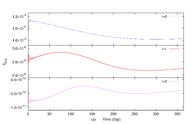
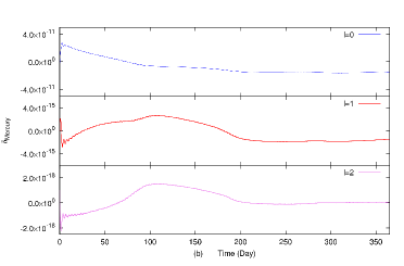
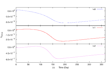
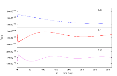
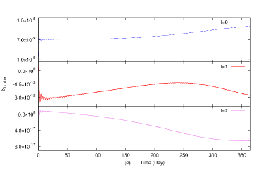
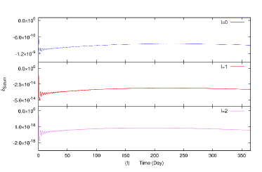
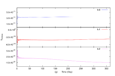
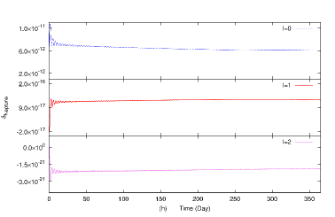
Figure 2: The normalized relative deviation between the analytic and numerical results $\delta_{A}$ for perturbing bodies with $l=0$ (blue),$l=1$ (red),$l=2$ (violet) versus the integral time (in days). (a) for the Sun; (b) for Mercury; (c) for Venus; (d) for the EMB; (e) for Jupiter; (f) for Saturn; (g) for Uranus; (h) for Neptune.

Figure 3: Left:The normalized relative deviation for Mars versus the integral time (in days). Right: The normalized relative deviation for the velocity of the spacecraft in the BCRS versus the integral time (in days).

With these numerical results, we can check our analytic approach. Firstly, we consider the effects of the dynamical term. For perturbations, there are three terms in the analytic expression (see Eq. (12)). We introduce a dimensionless quantity $\delta_{A}$ for contribution A in $\tau_{s}-t$, which is defined as $\delta_{A}\equiv[\mathrm{analytic~{}(A})-\mathrm{numerical~{}(A})]/[\mathrm{numerical}~{}(\tau_{s}-t)]$. Fig. 2 shows $\delta_{A}$ of the Sun, Mercury, Venus, EMB, Jupiter, Saturn, Uranus and Neptune for $l=0$, $l=1$ and $l=2$. The contributions of perturbations are very well described by our analytic approach because $\delta_{A}$ decreases to $\sim 10^{-12}$ or below with $l=2$. Although the curves of Fig. 2 have some fluctuation in the beginning, they tend to be smooth with time. For the effect of Mars in the dynamical term, the left one of Fig. 3 displays the comparison between the numerical and the analytic results. The maximum $\delta_{\mathrm{Mars}}$ is about $10^{-7}$. The right one of Fig. 3 shows the numerical check of the kinematic term and $\delta_{v_{s}^{2}}$ is about $10^{-5}$. Both of them are caused by the fact that pure two-body problem solutions are adopted in our analytic approach but it is full N-body integration in the numerical simulation.

4 Analytic results

Figure 4: This figure shows the difference in $\tau_{s}-t$ with the time.

Table 1: Components in $\tau_{s}-t$

	Max (s)	Order		Max (s)	Order		Max (s)	Order
Sun	0.2	$c^{-2}$	Mercury	$4\times 10^{-8}$	$c^{-2}$	EMB	$4\times 10^{-7}$	$c^{-2}$
Sun	$7\times 10^{-10}$	$c^{-4}$	Venus	$6\times 10^{-7}$	$c^{-2}$	Mars	$3\times 10^{-4}$	$c^{-2}$
Jupiter	$7\times 10^{-5}$	$c^{-2}$	Uranus	$7\times 10^{-7}$	$c^{-2}$	$\int\frac{1}{2}v^{2}_{s}\mathrm{d}t$	0.1	$c^{-2}$
Saturn	$8\times 10^{-6}$	$c^{-2}$	Neptune	$5\times 10^{-7}$	$c^{-2}$	$\int\frac{1}{8}v^{4}_{s}\mathrm{d}t$	$2\times 10^{-10}$	$c^{-4}$

Figure 5: Different terms in Eq. (12) versus the time. Figures (a)-(j) denote the contributions from the Sun, Mercury, Venus, the EMB, Mars, Jupiter, Saturn, Uranus, Neptune and $v^{2}_{s}$ at the order of $c^{-2}$, respectively. Figures (k) and (l) denote the effects of the Sun and the velocity of the spacecraft in $\tau_{s}-t$ at the order of $c^{-4}$.

Some results are derived with our analytic method after qualified by the numerical check. Fig. 4 shows the curve of $\tau_{s}-t$ by Eq. (12). We can see the difference between the proper time and TCB could reach the level of sub-second. This effect has two main components: the Sun’s gravitational field and the velocity of the spacecraft in the BCRS. Fig.5(a)-(j) display the contributions of the Sun, Mercury, Venus, the EMB, Mars, Jupiter, Saturn, Uranus, Neptune and the velocity of the spacecraft (i.e. $-\epsilon^{2}\int v^{2}_{s}/2\mathrm{d}t$). Since the Sun’s gravitational field and the velocity of the spacecraft in BCRS dominate, we further consider these contribution in the next order, namely, $\epsilon^{4}\int G^{2}m^{2}_{\odot}/(2r^{2}_{s\odot})\mathrm{d}t$ and $-\epsilon^{4}\int v^{4}_{s}/8\mathrm{d}t$ (see Fig.3(k) and Fig.3(l)). These two terms in the order of $\epsilon^{4}$ are very small around $\sim 10^{-10}$s.

Table 1 gives the maximum values of different effects in the $\tau_{s}-t$. At the order of $\epsilon^{2}$, the Sun’s gravitational field and the velocity for the spacecraft have the contributions up to a few sub-seconds, while others belong to microsecond-level or below. At the order of $\epsilon^{4}$, the maximum contributions of the Sun’s gravitational field and the velocity for the spacecraft are at the level of $0.1$ nanosecond. It means if we take $1$ nanosecond as the precision of time system, the transformation between the proper time on the spacecraft and TCB needs to include the terms at the order of $\epsilon^{2}$ only.

If we take YingHuo-1 Mission as a technical example for Chinese future Mars explorations, the supposed spacecraft will be equipped with a clock such as the Ultra-Stable-Oscillator (USO), whose instability is less than $1\times 10^{-12}$ or $2\times 10^{-12}$ from 0.1 to 1000 seconds ([Ping et al. (2009)]). The accuracy control must be done for a clock carried on board because its accuracy will be drift as a result of various reasons. Thus, it is almost impossible to estimate the timing error of a clock after one year through its stability or accuracy number. And we only discuss a time span in one year mission such as one month. $\tau_{s}-t$ can get the level of $10^{-2}$s in one month. At the level of microsecond $10^{-6}$s of the time accuracy, although $\delta_{\mathrm{Mars}}$ and $\delta_{v_{s}^{2}}$ could reach $10^{-7}$ and $10^{-5}$ maximally, their maximum contributions in the deviation of $\tau_{s}-t$ are respectively $10^{-9}$s and $10^{-7}$s for one month, both of them less than $10^{-6}$s. It shows our analytical approach is qualified for a Mars orbiter.

5 Conclusion

In this paper, the transformation between the proper time on the spacecraft and TCB is derived under IAU resolutions. In order to obtain more clearly physical pictures and improve computational efficiency, an analytic approach is employed. A numerical simulation of a Mars mission is conducted and shows this approach is qualified, especially being good at dealing with perturbations. It shows that the difference between the proper time on the spacecraft and TCB reaches the level of sub-second. And the main contributions of this transformation come from the Sun’s gravitational field and the velocity of the spacecraft in the BCRS.

In this work, we only take two-body problem solutions, which makes the relative deviations of Mars’ gravitational field and the velocity of the spacecraft reach respectively about $10^{-7}$ and $10^{-5}$. Our next move is to include the effect of the three-body disturbing function of the spacecraft.

It is worthy of note that there is a long interplanetary journey for a spacecraft before the arrival at the target. In this case, the transformation between $\tau_{s}$ and TCB has exactly the same structure as the Eq.(13), and could be dramatically simplified as $\tau_{s}-t=-\epsilon^{2}\int(Gm_{\odot}/r_{s\odot}+v^{2}_{s}/2)\mathrm{d}t$ when the probe is far beyond the Hill sphere of any massive body except the Sun. Therefore, the final $\tau_{s}-t$ during this phase is strongly dependent on the trajectory the spacecraft takes. However, most of spacecrafts spend their time on this in the quiet mode until crucial orbital maneuvers or scientifically important flybys. For this reason, we do not take much care of this issue and it is easy to handle indeed.