Stochastic resonance in bistable systems with nonlinear dissipation and multiplicative noise: A microscopic approach

Abstract

The stochastic resonance (SR) in bistable systems has been extensively discussed with the use of phenomenological Langevin models. By using the microscopic, generalized Caldeira-Leggett (CL) model, we study in this paper, SR of an open bistable system coupled to a bath with a nonlinear system-bath interaction. The adopted CL model yields the non-Markovian Langevin equation with nonlinear dissipation and state-dependent diffusion which preserve the fluctuation-dissipation relation (FDR). From numerical calculations, we find the following: (1) the spectral power amplification (SPA) exhibits SR not only for $a$ and $b$ but also for $\tau$ while the stationary probability distribution function is independent of them where $a$ ($b$) denotes the magnitude of multiplicative (additive) noise and $\tau$ expresses the relaxation time of colored noise; (2) the SPA for coexisting additive and multiplicative noises has a single-peak but two-peak structure as functions of $a$, $b$ and/or $\tau$. These results (1) and (2) are qualitatively different from previous ones obtained by phenomenological Langevin models where the FDR is indefinite or not held.

I Introduction

In the last three decades since a seminal work of Benzi et. al. Benzi81 , extensive studies have been made on the stochastic resonance (SR) (for a recent review on SR, see Refs. Gamma98 ; Lindner04 ). Theoretical studies on SR were made initially with the use of the overdamped Langevin model subjected to white noise. It has been shown that the signal-to-noise ratio (SNR) of nonlinear systems to a small periodic signal is resonantly enhanced under some optimum level of noise, whose effect is called SR Gamma98 ; Lindner04 . The resonant activation occurs when the frequency of an applied periodic signal is near the Kramer escape rate of the transition from one potential minimum to another. Subsequent studies on SR examined effects of colored noise (for a review on colored noise, see Ref. Hanggi95 ). Calculations with the use of the universal colored-noise approximation (UCNA) Jung87 have shown that noise color suppresses SR monotonically with increasing its relaxation time $\tau$ Hanggi84 ; Hanggi93 ; Gamma89 . Ref. Neiman96 has claimed that when $\tau$ is increased, the SR is first suppressed for small $\tau$ but enhanced for large $\tau$ with the minimum at intermediate $\tau$. In recent years, studies on SR have been made by using more sophisticated noise: correlated additive white noise and multiplicative colored noise Li95 ; Fu99 ; Jia00 ; Jia01 ; Luo03 . SNR of the Langevin model subjected to such noises is shown to exhibit a complicated behavior as functions of magnitudes of additive and multiplicative noises and the correlation strength between the two noises Jia00 ; Jia01 ; Luo03 . For example, SNR may have the bimodal structure when these parameters are varied.

It should be noted that Langevin equations having been adopted for studies on SR are phenomenological ones which have some deficits such that a lack of the fluctuation-dissipation relation (FDR), related discussion being given in Sec. IV. We expect that in almost all real, non-isolated systems, the environment acts as a thermal bath which is a source of noise. The microscopic origin of additive noise has been proposed within a framework of Caldeira-Leggett (CL) system-bath Hamiltonian Ford65 ; Ullersma66 ; Caldeira81 . The CL model with a linear system-bath coupling leads to the non-Markovian Langevin equation where memory kernel and noise term are expressed in terms of bath variables and they satisfy the FDR Ford65 ; Ullersma66 ; Caldeira81 . The FDR implies that dissipation and diffusion come from the same origin. By using the generalized CL model including a nonlinear system-bath coupling, we may obtain the non-Markovian Langevin equation with multiplicative noise which preserves the FDR Lindenberg81 ; Pollak93 . The nature of nonlinear dissipation and multiplicative noise has been recently explored with renewed interest Barik05 ; Plyukhin07 ; Farias09 . Nonlinear dissipation and multiplicative noise have been recognized as important ingredients in several fields such as mesoscopic scale systems Zaitsev09 ; Eichler11 and ratchet problems Magnasco93 ; Julicher97 ; Reimann02 ; Porto00 .

Quite recently, we have studied the generalized CL model for a harmonic oscillator which includes nonlinear nonlocal dissipation and multiplicative diffusion Hasegawa11d . It has been shown that the stationary probability distribution function (PDF) is independent of magnitudes of additive and multiplicative noises and of the relaxation time of colored noise Barik05 ; Plyukhin07 ; Farias09 ; Hasegawa11d , although the response to applied input depends on noise parameters Hasegawa11d . This is in contrast with previous studies Sakaguchi01 ; Anteneodo03 ; Hasegawa07 which show that the stationary PDF of the Langevin model for the harmonic potential is Gaussian or non-Gaussian, depending on magnitudes of additive and multiplicative noises. We expect that when the generalized CL model with a nonlinear coupling Barik05 ; Plyukhin07 ; Farias09 ; Hasegawa11d is applied to a bistable system, properties of the calculated SR may be rather different from those having been derived by the phenomenological Langevin models Hanggi84 ; Hanggi93 ; Hanggi95 ; Gamma89 ; Neiman96 ; Li95 ; Fu99 ; Jia00 ; Jia01 ; Luo03 . It is the purpose of the present paper to make a detailed study on SR of an open bistable system described by the microscopic, generalized CL model with nonlinear nonlocal dissipation and state-dependent diffusion Hasegawa11d . Although the UCNA has been employed in many studies on SR for colored noise Li95 ; Fu99 ; Jia00 ; Jia01 ; Luo03 because it is exact both for $\tau=0.0$ and $\tau=\infty$ Jung87 , its validity within $O(\tau)$ is not justified Timmermann01 ; Hasegawa07b . In this study, we investigate SR for a wide range of $\tau$ value by simulations.

The paper is organized as follows. In Sec. II, we briefly summarize the non-Markovian Langevin equation derived from the generalized CL model with OU colored noise Barik05 ; Plyukhin07 ; Farias09 ; Hasegawa11d . In Sec. III, after studying the stationary PDF, we investigate SR of an open bistable system for three cases: additive noise, multiplicative noise, and coexisting additive and multiplicative noises. In Sec. IV, we examine a validity of the Markovian Langevin equations with the local approximation, which have been widely employed in previous studies on SR Hanggi84 ; Hanggi93 ; Hanggi95 ; Gamma89 . Sec. V is devoted to our conclusion.

II The generalized CL model

II.1 Non-Markovian Langevin equation

We consider a system of a Brownian particle coupled to a bath consisting of $N$-body uncoupled oscillators, which is described by the generalized CL model Barik05 ; Plyukhin07 ; Farias09 ; Hasegawa11d ,

$$H = H_{S}+H_{B}+H_{I},$$ (1)

with

$$H_{S} = \frac{p^{2}}{2}+V(x)-xf(t),$$ (2)

$$H_{B}+H_{I} = \sum_{n=1}^{N}\left\{\frac{p_{n}^{2}}{2m_{n}}+\frac{m_{n}\omega_{n}^{2}}{2}\left(q_{n}-\frac{c_{n}\phi(x)}{m_{n}\omega_{n}^{2}}\right)^{2}\right\}.$$ (3)

Here $H_{S}$, $H_{B}$ and $H_{I}$ express Hamiltonians of the system, bath and interaction, respectively; $x$, $p$ and $V(x)$ denote position, momentum and potential, respectively, of the system; $q_{n}$, $p_{n}$, $m_{n}$ and $\omega_{n}$ stand for position, momentum, mass and frequency, respectively, of bath; the system couples to the bath nonlinearly through a function $\phi(x)$; $f(t)$ expresses an applied external force. The original CL model adopts a linear system-bath coupling with $\phi(x)=x$ in Eq. (3) which yields additive noise Caldeira81 . By using the standard procedure, we obtain the generalized Langevin equation given by Caldeira81 ; Lindenberg81 ; Pollak93 ; Barik05 ; Hasegawa11d

$$\ddot{x}(t) = -V^{\prime}(x(t))-\phi^{\prime}(x(t))\int_{0}^{t}\gamma(t-t^{\prime})\>\phi^{\prime}(x(t^{\prime}))\>\dot{x}(t^{\prime})\>dt^{\prime}+\phi^{\prime}(x(t))\>\zeta(t)+f(t),$$ (4)

with

$$\gamma(t) = \sum_{n=1}^{N}\left(\frac{c_{n}^{2}}{m_{n}\omega_{n}^{2}}\right)\cos\omega_{n}t,$$ (5)

$$\zeta(t) = \sum_{n=1}^{N}\left\{\left[\frac{m_{n}\omega_{n}^{2}}{c_{n}}\>q_{n}(0)-\phi(x(0))\right]\left(\frac{c_{n}^{2}}{m_{n}\omega_{n}^{2}}\right)\cos\omega_{n}t+\left(\frac{c_{n}p_{n}(0)}{m_{n}\omega_{n}}\right)\sin\omega_{n}t\right\},$$ (6)

where $\gamma(t-t^{\prime})$ denotes the non-local memory kernel and $\zeta(t)$ stands for noise, and dot and prime stand for derivatives with respect to time and argument, respectively. Dissipation and diffusion terms given by Eqs. (5) and (6), respectively, satisfy the FDR,

$$\left<\zeta(t)\zeta(t^{\prime})\right>_{0} = k_{B}T\>\gamma(t-t^{\prime}),$$ (7)

where the bracket $\langle\cdot\rangle_{0}$ stands for the average over initial states of $q_{n}(0)$ and $p_{n}(0)$ Lindenberg81 ; Pollak93 ; Barik05 .

We adopt the OU process for the kernel $\gamma(t-t^{\prime})$ given by

$$\gamma(t-t^{\prime}) = \left(\frac{\gamma_{0}}{\tau}\right)e^{-|t-t^{\prime}|/\tau},$$ (8)

where $\gamma_{0}$ and $\tau$ stand for the strength and relaxation time, respectively, of colored noise. The OU colored noise may be generated by the differential equation,

$$\dot{\zeta}(t) = -\frac{\zeta(t)}{\tau}+\frac{\sqrt{2k_{B}T\gamma_{0}}}{\tau}\>\xi(t),$$ (9)

where $\xi(t)$ expresses white noise with

$$\left<\xi(t)\right> = 0,\;\;\;\;\left<\xi(t)\xi(t^{\prime})\right>=\delta(t-t^{\prime}).$$ (10)

Equations (9) and (10) lead to the PDF and correlation of colored noise given by

$$P(\zeta) \propto e^{-(\beta\tau/2\gamma_{0})\>\zeta^{2}},$$ (11)

$$\left<\zeta(t)\zeta(t^{\prime})\right> = \left(\frac{k_{B}T\gamma_{0}}{\tau}\right)\>e^{-|t-t^{\prime}|/\tau}=k_{B}T\>\gamma(t-t^{\prime}),$$ (12)

where $\beta=1/k_{B}T$.

In order to transform the non-Markovian Langevin equation given by Eq. (4) into more tractable multiple differential equations, we introduce a new variable $u(t)$ Pollak93 ; Farias09 ,

$$u(t) = -\int_{0}^{t}\gamma(t-t^{\prime})\phi^{\prime}(x(t^{\prime}))\dot{x}(t^{\prime})\>dt^{\prime},$$ (13)

which yields four first-order differential equations for $x(t)$, $p(t)$, $u(t)$ and $\zeta(t)$ given by

$$\dot{x}(t) = p(t),$$ (14)

$$\dot{p}(t) = -V^{\prime}(x)+\phi^{\prime}(x(t))\>u(t)+f(t)+\phi^{\prime}(x(t))\>\zeta(t),$$ (15)

$$\dot{u}(t) = -\frac{u(t)}{\tau}-\left(\frac{\gamma_{0}}{\tau}\right)\phi^{\prime}(x(t))\>p(t),$$ (16)

$$\dot{\zeta}(t) = -\frac{\zeta(t)}{\tau}+\frac{\sqrt{2k_{B}T\gamma_{0}}}{\tau}\>\xi(t).$$ (17)

From Eqs. (14)-(17), we obtain the multi-variate Fokker-Planck equation (FPE) for distribution of $P(x,p,u,\zeta,t)$,

$$\frac{\partial P(x,p,u,\zeta,t)}{\partial t} = -\frac{\partial}{\partial x}\>p\>P(x,p,u,\zeta,t)$$ (18)

$$- \frac{\partial}{\partial p}\left[-V^{\prime}(x)+f(t)+\phi^{\prime}(x)u+\phi^{\prime}(x)\zeta\right]P(x,p,u,\zeta,t)$$

$$- \frac{\partial}{\partial u}\left[\frac{u}{\tau}+\left(\frac{\gamma_{0}}{\tau}\right)\>\phi^{\prime}(x)p\right]P(x,p,u,\zeta,t)+\frac{\partial}{\partial\zeta}\left(\frac{\zeta}{\tau}\right)P(x,p,u,\zeta,t)$$

$$+ \left(\frac{k_{B}T\gamma_{0}}{\tau^{2}}\right)\frac{\partial^{2}}{\partial\zeta^{2}}P(x,p,u,\zeta,t).$$

The stationary PDF with $f(t)=0$ is given by Pollak93

$$P(x,p) = \int P(x,p,u,\zeta)\;du\;d\zeta\propto e^{-\beta[p^{2}/2+V(x)]}.$$ (19)

II.2 Markovian Langevin equation

It is worthwhile to examine the local limit of Eq. (7),

$$\left<\zeta(t)\zeta(t^{\prime})\right>_{0} = k_{B}T\>\gamma(t-t^{\prime})=2k_{B}T\>\gamma_{0}\>\delta(t-t^{\prime}),$$ (20)

which leads to the Markovian Langevin equation given by

$$\ddot{x}(t) = -V^{\prime}(x(t))-\gamma_{0}\phi^{\prime}(x(t))^{2}\>\dot{x}(t)+\sqrt{2k_{B}T}\>\phi^{\prime}(x)\>\xi(t)+f(t),$$ (21)

preserving the FDR. It is evident that the Markovian Langevin equation becomes a good approximation of the non-Markovian one in the limit of $\tau\rightarrow 0$.

From Eq. (21), we obtain first-order differential equations,

$$\dot{x}(t) = p(t),$$ (22)

$$\dot{p}(t) = -V^{\prime}(x)-\gamma_{0}\phi^{\prime}(x(t))^{2}p(t)+\sqrt{2k_{B}T\gamma_{0}}\;\phi^{\prime}(x(t))\>\xi(t)+f(t).$$ (23)

The relevant FPE for the PDF of $P(x,p,t)$ is expressed by

$$\frac{\partial P(x,p,t)}{\partial t} = -\frac{\partial}{\partial x}\>p\>P(x,p,t)+\frac{\partial}{\partial p}\left[V^{\prime}(x)-f(t)+\gamma_{0}\phi^{\prime}(x)^{2}\>p\right]P(x,p,t)$$ (24)

$$+ k_{B}T\>\gamma_{0}\;\frac{\partial}{\partial p}\phi^{\prime}(x)\frac{\partial}{\partial p}\phi^{\prime}(x)P(x,p,t).$$

The stationary distribution of Eq. (24) with $f(t)=0$ is given by

$$P(x,p) \propto \>e^{-\beta[p^{2}/2+V(x)]},$$ (25)

which is consistent with the result of the non-Markovian Langevin equation given by Eq. (19).

II.3 Overdamped Langevin equation

We will derive the overdamped Langevin equation from the Markovian Langevin model given by Eq. (21). The overdamped limit of the Markovian Langevin equation is conventionally derived with setting $\ddot{x}=0$ in Eq. (21). This is, however, not the case because dissipation and diffusion terms are state dependent in Eq. (21). Sancho, San Miguel and Dürr Sancho82 have developed an adiabatic elimination procedure to obtain an exact overdamped Langevin equation and its FPE. In order to adopt their method Sancho82 , we rewrite Eq. (21) as

$$\ddot{x}(t) = -V^{\prime}(x(t))-\lambda(x(t))\dot{x}(t)+g(x(t))\>\xi(t)+f(t),$$ (26)

with

$$\lambda(x) = \gamma_{0}\phi^{\prime}(x)^{2},$$ (27)

$$g(x) = \sqrt{2k_{B}T\gamma_{0}}\>\phi^{\prime}(x).$$ (28)

By the adiabatic elimination in Eq. (26) after Ref. Sancho82 , the FPE in the Stratonovich interpretation is given by

$$\frac{\partial P(x,t)}{\partial t} = \frac{\partial}{\partial x}\frac{1}{\lambda(x)}\left[V^{\prime}(x)-f(t)+k_{B}T\frac{\partial}{\partial x}\right]P(x,t),$$ (29)

where we employ the relation: $g(x)^{2}=2k_{B}T\lambda(x)$ derived from Eqs. (27) and (28). The relevant Langevin equation is given by Sancho82

$$\dot{x} = -\frac{[V^{\prime}(x)-f(t)]}{\lambda(x)}-\frac{1}{2\lambda(x)^{2}}\>g^{\prime}(x)g(x)+\frac{g(x)}{\lambda(x)}\>\xi(t).$$ (30)

Note that the second term of Eq. (30) does not appear when we obtain the overdamped Langevin equation by simply setting $\ddot{x}=0$ in Eq. (26). It is easy to see that the stationary distribution of Eq. (29) with $f(t)=0$ is given by

$$P(x) \propto e^{-\beta V(x)}.$$ (31)

III Bistable systems

III.1 Stationary PDF

We apply the generalized CL model mentioned in the preceding section to a bistable system, where $V(x)$ and $\phi(x)$ in Eqs. (1)-(3) are given by

$$V(x) = \frac{x^{4}}{4}-\frac{x^{2}}{2},$$ (32)

$$\phi(x) = \frac{ax^{2}}{2}+bx\hskip 28.45274pt\mbox{($a\geq 0,\;b\geq 0$)},$$ (33)

$a$ and $b$ denoting magnitudes of multiplicative and additive noises, respectively. The symmetric bistable potential given by Eq. (32) has two stable minima at $x=\pm 1.0$ and unstable maximum at $x=0.0$. The height of the potential barrier is given by $\Delta\equiv V(0)-V(\pm 1)=1/4$.

First we show calculations of the stationary PDF. We have solved Eqs. (14)-(17) by using the Heun method Note1 ; Note2 with a time step of 0.001 for parameters of $\gamma_{0}=1.0$ and $k_{B}T=\Delta=0.25$. Simulations of Eqs. (14)-(17) have been performed for $0\leq t<1000.0$ with discarding initial results at $t<200.0$. Calculated results to be reported are averaged over $10\;000$ runs with initial states of Gaussian-distributed $x(0)$, $p(0)$ and $\zeta(0)$ with $\langle x(0)\rangle=\langle p(0)\rangle=\langle\zeta(0)\rangle=0$, $\langle x(0)^{2}\rangle=\langle p(0)^{2}\rangle=k_{B}T$, and $\langle\zeta(0)^{2}\rangle=k_{B}T\gamma_{0}/\tau$. An initial condition of $u(0)=0$ has been used in all simulations.

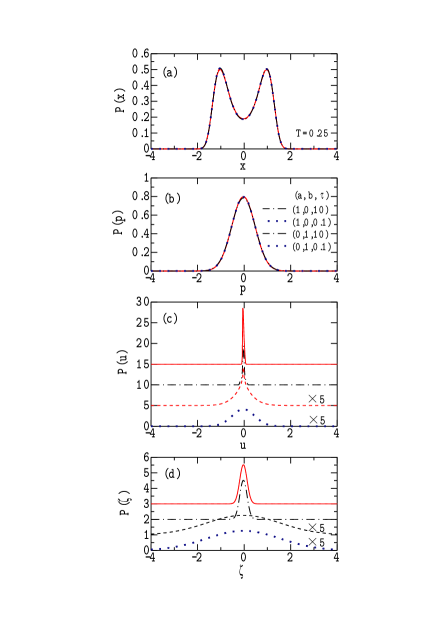
Figure 1: (Color online) Marginal PDFs of (a) $P(x)$, (b) $P(p)$, (c) $P(u)$ and (d) $P(\zeta)$ for $(a,b,\tau)=(1,0,10.0)$ (solid curves), $(1,0,0.1)$ (dashed curves), $(0,1,10.0)$ (chain curves), and $(0,1,0.1)$ (dotted curves) calculated by simulations with $\gamma_{0}=1.0$ and $k_{B}T=\Delta=0.25$. $P(x)$ and $P(p)$ in (a) and (b) are indistinguishable among the four sets of $(a,b,\tau)$. $P(u)$ and $P(\zeta)$ for $(a,b,\tau)=(1,0,0.1)$ and (0,1,0.1) are multiplied by a factor of five in (c) and (d) where PDFs are arbitrarily shifted for a clarity of figures.

Calculated marginal PDFs of $P(x)$, $P(p)$, $P(u)$ and $P(\zeta)$ for $f(t)=0$ are shown in Figs. 1(a), (b), (c) and (d), respectively, where four sets of parameters are adopted: $(a,b,\tau)=(1,0,10.0)$ (solid curves), $(1,0,0.1)$ (dashed curves), $(0,1,10.0)$ (chain curves) and $(0,1,0.1)$ (dotted curves). We note that $P(x)$ and $P(p)$ in Figs. 1(a) and (b) are independent of the parameters of $(a,b,\tau)$ although $P(u)$ and $P(\zeta)$ in Figs. 1(c) and (d) depend on them. Calculated $P(x)$ and $P(p)$ are in good agreement with marginal PDFs obtained by

$$P(x) = \int P(x,p)\;dp\propto e^{-\beta V(x)},$$ (34)

$$P(p) = \int P(x,p)\;dx\propto e^{-\beta p^{2}/2},$$ (35)

which show that $P(x)$ has the typical bimodal structure while $P(p)$ is Gaussian. Equation (11) shows that $P(\zeta)$ is the Gaussian PDF whose variance depends on $\tau$ for fixed $\gamma_{0}$ and $T$. In contrast, Fig. 1(c) shows that $P(u)$ is Gaussian PDF for additive noise but non-Gaussian PDF for multiplicative noise. Properties of stationary PDFs for bistable potential shown in Fig. 1 are similar to those for harmonic oscillators except for $P(x)$ (see Fig. 1 of Ref. Hasegawa11d ).

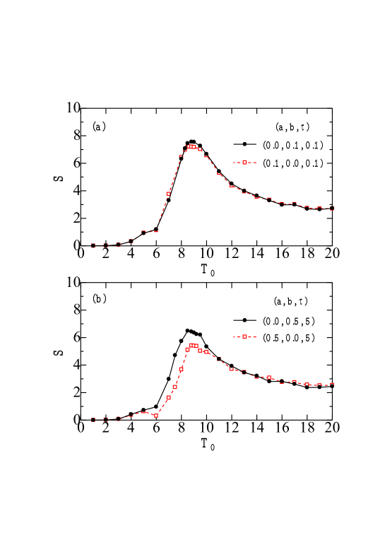
Figure 2: (Color online) (a) SPA ($S$) as a function of a period of an input ($T_{0}$) for $(a,b,\tau)=(0.0,0.1,0.1)$ (solid curve) and $(0.1,0.0,0.1)$ (dashed curve). (b) $S$ as a function of $T_{0}$ for $(a,b,\tau)=(0.0,0.5,5.0)$ (solid curve) and $(0.5,0.0,5.0)$ (dashed curve).

III.2 Stochastic resonance

III.2.1 Spectral power amplification

We investigate SR, applying a sinusoidal input given by

$$f(t) = g\>\cos\left(\frac{2\pi t}{T_{0}}\right)=g\>\cos\omega_{0}t,$$ (36)

where $g$, $T_{0}$ and $\omega_{0}$ ($=2\pi/T_{0}$) denote its magnitude, period and frequency, respectively. A sinusoidal input given by Eq. (36) yields an averaged output given by

$$\mu(t) = \langle x(t)\rangle,$$ (37)

where $\langle\cdot\rangle$ denotes the average over trials. We evaluate the spectral power amplification (SPA) $S$ defined by

$$S = \frac{|\>\mu[\omega_{0}]\>|^{2}}{|\>f[\omega_{0}]\>|^{2}},$$ (38)

where $f[\omega]$ and $\mu[\omega]$ are Fourier transformations of $f(t)$ and $\mu(t)$, respectively. Simulation procedures are the same as those for a calculation of stationary PDFs except for initial conditions of $x(0)$ and $p(0)$ which are taken to be $x(0)=1.0$ and $p(0)=0.0$. Direct simulations for Eqs. (14)-(17) have been made for sets of $a$, $b$, $\tau$, $g$ and $T_{0}$ averaged over $10\;000$ runs.

Figure 2(a) shows SPA ($S$) as a function of a period of an external input ($T_{0}$) with $g=0.05$ for two sets of parameters: $(a,b,\tau)=(0.0,0.1,0.1)$ (solid curve) and $(0.1,0.0,0.1)$ (dashed curve), the former (latter) corresponding to additive (multiplicative) noise only. SPAs for both sets of parameters have maxima at $T_{0}\sim 9$. It is interesting that $S$ for additive noise nearly coincides with that for multiplicative noise. This coincidence, however, is not realized for a larger $\tau$ and/or $b$ as shown in Fig. 2(b) where similar plots of the $T_{0}$ dependence of $S$ are presented for different two sets of parameters: $(a,b,\tau)=(0.0,0.5,5)$ (solid curve) and $(0.5,0.0,5)$ (dashed curve). Resonances of $S$ in Fig. 2(b) are again realized at about $T_{0}\sim 9$ which coincides with the result in Fig. 2(a). This arises from the fact that an increase in the inverse of the Kramers rate with an increase of $\tau$ from $\tau=0.1$ to $\tau=5.0$ is approximately compensated by its decrease with an increase of $b$ from $b=0.1$ to $b=0.5$. Figures 2(a) and 2(b) clearly show the resonant behavior of $S$ when a period of an external sinusoidal input $T_{0}$ is varied. In the following, we will separately present simulation results for three cases: additive noise, multiplicative noise, and coexisting additive and multiplicative noises with fixed values of $T_{0}=10.0$ and $g=0.05$.

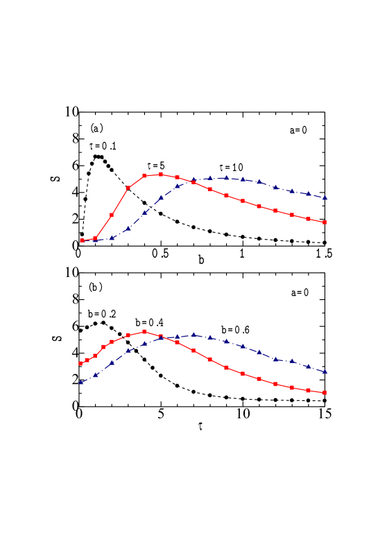
Figure 3: (Color online) (a) SPA $S$ for additive colored noise as a function of $b$ with $\tau=0.1$ (dashed curve), $\tau=5.0$ (solid curve) and $\tau=10.0$ (chain curve). (b) $S$ as a function of $\tau$ with $b=0.2$ (dashed curve), $b=0.4$ (solid curve) and $b=0.6$ (chain curve) ($a=0.0$, $g=0.05$ and $T_{0}=10.0$).

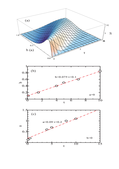
Figure 4: (Color online) (a) A schematic plot of $S$ as functions of $b$ and $\tau$ ($a$ and $\tau$) for additive (multiplicative) noise. (b) Locations of $S_{max}$ for additive colored noise in the $b$-$\tau$ plane obtained by simulations (circles), the chain line being expressed by $b=0.075\tau+0.1$. (c) Locations of $S_{max}$ for multiplicative colored noise in the $a$-$\tau$ plane obtained by simulations (circles), the chain line being expressed by $a=0.09\tau+0.2$.

III.2.2 Case of additive colored noise

First we apply only additive colored noise ($a=0.0$) to the system. Figure 3(a) shows SPA as a function of $b$ for $\tau=0.1$ (dashed curve), $\tau=5.0$ (solid curve) and $\tau=10.0$ (dashed curve). With increasing $\tau$, the $b$ value where $S$ has the maximum is increased, and the maximum value of $S$ ($S_{max}$) is gradually decreased with the wider distribution of $S$. Figure 3(b) shows the $\tau$ dependence of $S$ calculated for $b=0.2$ (dashed curve), $b=0.4$ (solid curve) and $b=0.6$ (dashed curve). $S_{max}$ in Figs. 3(a) and 3(b) is observed at a larger $b$ for a larger $\tau$ and vice versa.

Figure 4(a) shows a schematic plot of $S$ as functions of $b$ and $\tau$, which is estimated from simulation results shown in Figs. 3(a) and 3(b). We note that with increasing $b$ or $\tau$, a location of $S_{max}$ departs from the origin of $(b,\tau)=(0.0,0.0)$ and the magnitude of $S_{max}$ is gradually decreased. Circles in Fig. 4(b) denote locations of $S_{max}$ in the $b$-$\tau$ plane obtained by simulations shown in Figs. 3(a) and (b). $S_{max}$ nearly locates along the chain curve expressed by $b=0.075\tau+0.1$. Fig. 4(c) will be explained shortly.

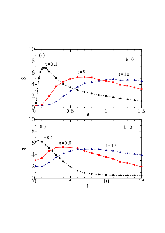
Figure 5: (Color online) (a) SPA $S$ for multiplicative colored noise as a function of $a$ with $\tau=0.1$ (dashed curve), $\tau=5.0$ (solid curve) and $\tau=10.0$ (chain curve). (b) $S$ as a function of $\tau$ with $a=0.2$ (dashed curve), $a=0.6$ (solid curve) and $a=1.0$ (chain curve) ($b=0.0$, $g=0.05$ and $T_{0}=10.0$).

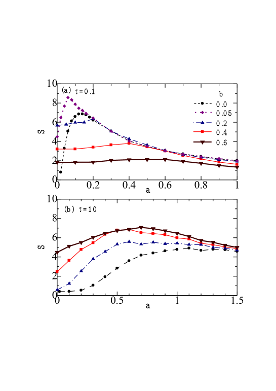
Figure 6: (Color online) SPA $S$ for coexisting additive and multiplicative colored noises with (a) $\tau=0.1$ and (b) $\tau=10.0$: $b=0.0$ (dashed curves), $b=0.05$ (dotted curves), $b=0.2$ (chain curves), $b=0.4$ (solid curves), and $b=0.6$ (bold solid curve) ($g=0.05$ and $T_{0}=10.0$).

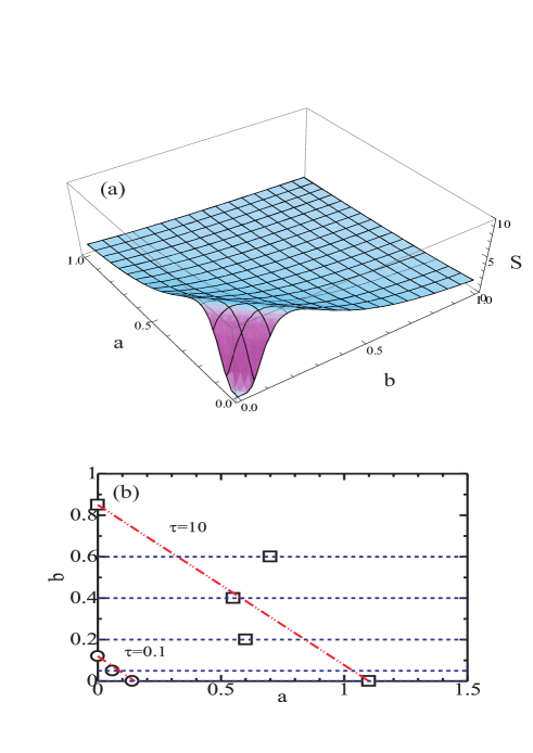
Figure 7: (Color online) (a) A schematic plot of $S$ as functions of $a$ and $b$ for coexisting additive and multiplicative noises. (b) Locations of $S_{max}$ in the $a$-$b$ plane: circles and squares denote $S_{max}$ for $\tau=0.1$ and $\tau=10.0$, respectively, obtained by simulations, chain and double-chain curves being shown for a guide of the eye. Along dashed lines, $a$ value in Fig. 6(a) or 6(b) is changed for a given $b$.

III.2.3 Case of multiplicative colored noise

Figure 5(a) shows the $a$ dependence of $S$ when we apply only multiplicative colored noise with $\tau=0.1$ (dashed curve), $\tau=5.0$ (solid curve) and $\tau=10.0$ (dashed curve). With increasing $\tau$, the position of $S_{max}$ moves to a larger $a$ and $S_{max}$ is gradually decreased. Figure 5(b) shows the $\tau$ dependence of $S$ calculated for $a=0.2$ (dashed curve), $a=0.6$ (solid curve) and $b=1.0$ (dashed curve).

We expect from simulation results in Figs. 5(a) and 5(b) that the $a$- and $\tau$-dependent PSA is given by Fig. 4(a) where we read the $b$ axis as the $a$ axis. As in the case where additive colored noise is added, a location of $S_{max}$ departs from the origin of $(a,\tau)=(0.0,0.0)$ and $S_{max}$ is gradually decreased with increasing $a$ or $\tau$. Circles in Fig. 4(c) denote locations of $S_{max}$ in the $a$-$\tau$ plane obtained by simulations shown in Figs. 5(a) and (b). $S_{max}$ nearly locates along the chain curve expressed by $a=0.09\tau+0.2$.

III.2.4 Case of coexisting additive and multiplicative colored noises

Next we study the case where both additive and multiplicative colored noises are applied to the system. Figure 6(a) shows the $a$ dependence of $S$ for $\tau=0.1$ with $b=0.0$ (dashed curves), $b=0.05$ (dotted curve), $b=0.2$ (chain curves) and $b=0.4$ (solid curves). The dashed curve for $b=0.0$ shows that $S$ has the maximum at $a\simeq 0.14$, as having been shown in Fig. 5(a). With adding small additive noise of $b=0.05$, $S_{max}$ is increased and its location moves to a smaller value of $a\simeq 0.05$. With further increase of $b$ ($\geq 0.2$), however, the magnitude of $S$ is gradually decreased and its maximum becomes obscure. A similar $a$ dependence of $S$ for $\tau=10.0$ is plotted in Fig. 6(b) where $S$ is monotonously increased with increasing $b$.

Figure 7(a) expresses a schematic plot of $S$ as functions of $a$ and $b$ for the case of coexisting additive and multiplicative noises, which are estimated from results of simulations shown in Figs. 6(a) and 6(b). $S$ has a small value at the origin of $(a,b)=(0.0,0.0)$. With departing from the origin by increases of $a$ and/or $b$, $S$ is first increased and then decreased after passing the maximum. Circles and squares in Fig. 7(b) denote locations of $S_{max}$ in the $a$-$b$ plane obtained for $\tau=0.1$ and $\tau=10.0$, respectively, from Figs. 6(a) and 6(b). $S_{max}$ nearly locates along a chain (double-chain) curve for $\tau=0.1$ ($\tau=10.0$): in the case of $\tau=10.0$ locations of $S_{max}$ are scattered because maximum of $S$ become obscure [Fig. 6(b)].

Dashed lines in Fig. 7(b) express traces along which $a$ value is changed for a given $b$ in Figs. 6(a) and 6(b). With increasing $b$ in Fig. 6(a) for $\tau=0.1$, the magnitude of $a$-dependent $S$ is decreased because a dashed line departs from the maximum expressed by a chain curve in Fig. 7(b), except for $b=0.05$ for which the $a$-dependent $S$ is increased. In contrast, with increasing $b$ in Fig. 6(b) for $\tau=10.0$, the magnitude of the $a$-dependent $S$ is increased, particularly for $a<0.5$, because a dashed line approaches the maximum expressed by a double-chain curve in Fig. 7(b). These explain the difference of the $b$ dependences of $S$ in Figs. 7(a) and 7(b).

IV Discussion

IV.1 Underdamped Markovian approximation for additive noise

We will examine the local approximation to the non-Markovian Langevin equation given by Eq. (4) for additive colored noise with $\phi^{\prime}(x)=b$,

$$\ddot{x} = -V^{\prime}(x)-b^{2}\int_{0}^{t}\gamma(t-t^{\prime})\>\dot{x}(t^{\prime})\>dt^{\prime}+b\>\zeta(t)+f(t),$$ (39)

where the nonlocal kernel and OU colored noise are given by

$$\langle\zeta(t)\zeta(t^{\prime})\rangle = k_{B}T\>\gamma(t-t^{\prime})=\left(\frac{k_{B}T\gamma_{0}}{\tau}\right)\>e^{-|t-t^{\prime}|/\tau}.$$ (40)

As mentioned in Sec. II B, when employing the local limit given by Eq. (20),

$$\left<\zeta(t)\zeta(t^{\prime})\right> = k_{B}T\>\gamma(t-t^{\prime})=2k_{B}T\>\gamma_{0}\>\delta(t-t^{\prime}),$$ (41)

we obtain the Markovian Langevin equation given by

$$\ddot{x} = -V^{\prime}(x)-b^{2}\gamma_{0}\>\dot{x}+\sqrt{2k_{B}T}\>b\>\xi(t)+f(t),$$ (42)

where $\xi(t)$ denotes white noise given by Eq. (10). If an alternative local approximation given by

$$\gamma(t-t^{\prime}) = 2\gamma_{0}\>\delta(t-t^{\prime}),\;\;\langle\zeta(t)\zeta(t^{\prime})\rangle=\left(\frac{k_{B}T\gamma_{0}}{\tau}\right)\>e^{-|t-t^{\prime}|/\tau},$$ (43)

is adopted, Eq. (39) reduces to the Markovian Langevin equation given by

$$\ddot{x} = -V^{\prime}(x)-b^{2}\gamma_{0}\>\dot{x}+b\>\zeta(t)+f(t).$$ (44)

We should note that the memory kernel and colored noise given by Eq. (43) do not satisfy the FDR for $\tau\neq 0.0$, while those given by Eqs. (40) and (41) hold the FDR. The Markovian Langevin equation given by Eq. (44) with OU colored noise [Eq. (43)] has been employed for a study on SR in Ref. Gamma89 .

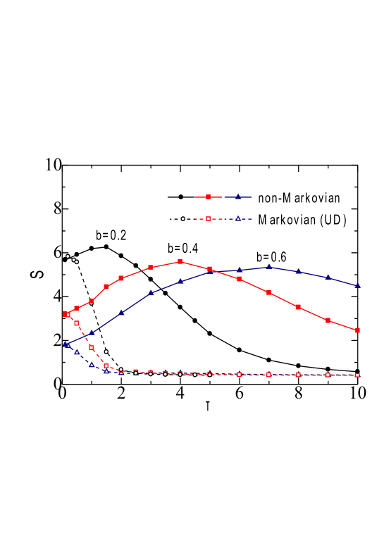
Figure 8: (Color online) The $\tau$ dependence of $S$ for additive noise ($a=0.0$) calculated by non-Markovian Langevin equation [Eq. (39)] (solid curves) and underdamped (UD) Markovian approximation [Eq. (44)] (dashed curves) with $b=0.2$ (circles), $b=0.4$ (squares) and $b=0.6$ (triangles) ($g=0.05$ and $T_{0}=10.0$).

Solid curves in Fig. 8 show the $\tau$ dependence of $S$ calculated by the non-Markovian Langevin equation [Eq. (39)] for $b=0.2$ (circles), 0.4 (squares) and 0.6 (triangle) with $k_{B}T=0.25$, $\gamma_{0}=1.0$, $g=0.05$ and $T_{0}=10.0$, which show the maxima as having been explained in Fig. 3(b). Dashed curves express relevant plots of $S$ for (underdamped) Markovian Langevin equation given by Eq. (44) with OU noise given [Eq. (43)]. At $\tau\rightarrow 0.0$, results of the Markovian approximation agree with those of the non-Markovian Langevin equation as expected. With increasing $\tau$, $S$ in the Markovian approximation monotonously decreased as shown in Ref. Gamma89 , although for $b=0.2$, $S$ is slightly increased at $0.1<\tau<0.4$ but decreased at $\tau>0.4$. It is evident that results of the Markovian Langevin equation given by Eq. (44) with the local approximation given by Eq. (43) are quite different from those of the non-Markovian Langevin equation given by Eq. (39) except for a very small $\tau$.

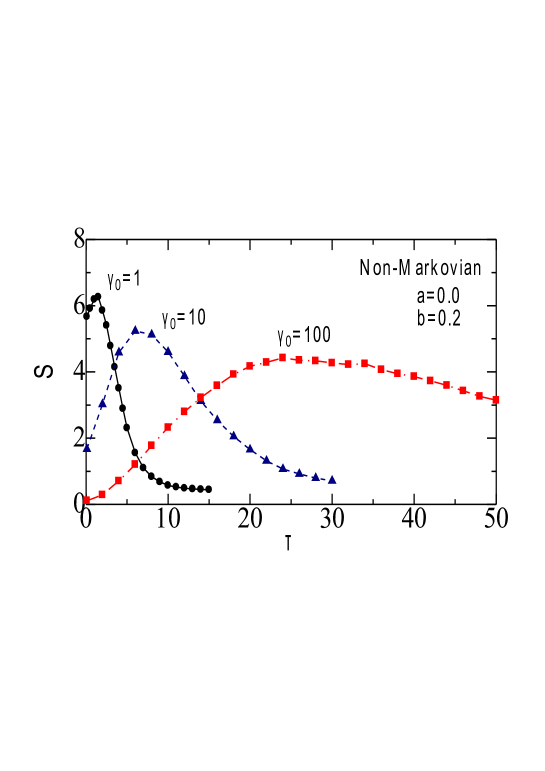
Figure 9: (Color online) The $\tau$ dependence of $S$ for additive noise calculated by the non-Markovian Langevin equation [Eq. (39)] for $\gamma_{0}=1.0$ (solid curve), $\gamma_{0}=10.0$ (dashed curve) and $\gamma_{0}=100.0$ (chain curve) with $a=0.0$, $b=0.2$, $g=0.05$ and $T_{0}=10.0$.

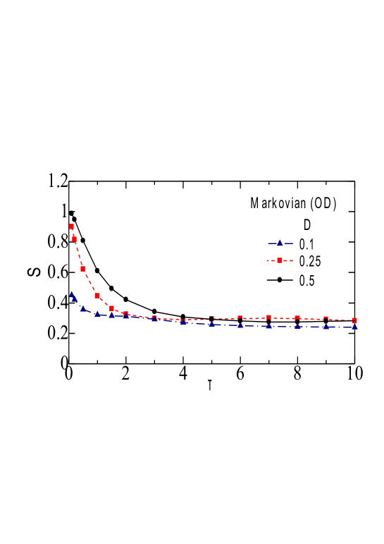
Figure 10: (Color online) The $\tau$ dependence of $S$ for additive noise calculated by the overdamped (OD) Markovian approximation [Eq. (45)] with $D=0.10$ (chain curve), $D=0.25$ (dashed curve) and $D=0.50$ (solid curve) (see text).

IV.2 Overdamped Markovian approximation for additive noise

In order to gain an insight into SR of the overdamped limit of the non-Markovian Langevin equation given by Eq. (39) subjected to additive noise, we have performed simulations, employing a large value of $\gamma_{0}$ in Eq. (40). Figure 9 shows the $\tau$ dependence of $S$ for $\gamma_{0}=1.0$ (solid curve), $10.0$ (dashed curve) and $100.0$ (chain curve) with $a=0.0$, $b=0.2$, $g=0.05$ and $T_{0}=10.0$. With a larger $\gamma_{0}$, $S(\tau)$ for $\tau\rightarrow 0$ becomes smaller and the peak position for $S_{max}$ becomes larger. $S$ for all the cases investigated has the maximum. Our calculation suggests that SR might be realized against $\tau$ even in the overdamped limit of the non-Markovian Langevin equation.

In previous studies Hanggi84 ; Hanggi93 , the overdamped Langevin equation given by

$$\dot{x} = -V^{\prime}(x)+\zeta(t)+f(t),$$ (45)

with the OU noise correlation.

$$\langle\zeta(t)\zeta(t^{\prime})\rangle=\left(\frac{D}{\tau}\right)\>e^{-|t-t^{\prime}|/\tau},$$ (46)

has been extensively studied within the UCNA. Equation (45) may be obtainable from Eq. (44) with setting $\ddot{x}=0$ and an appropriate change of variables.

Figure 10 shows the $\tau$ dependence of $S$ calculated by simulations for the overdamped Markovian Langevin equation given by Eq. (45) with OU colored noise [Eq. (46)] for $D=0.10$ (chain curve), 0.25 (dashed curve) and 0.50 (solid curve). With increasing $\tau$, all calculated results show monotonous decrease, in consistent with the result of the UCNA in Refs. Hanggi84 ; Hanggi93 . However, they exhibit no signs of the SR against $\tau$, which is in contrast with the result in Fig. 9 obtained by the non-Markovian Langevin equation for a large $\gamma_{0}$.

The discrepancy between results of non-Markovian Langevin equation [Eq. (39)] and Markovian Langevin equations [Eqs. (44) and (45)] whose results are presented in Figs. 8, 9 and 10, arises from the fact that the FDR is preserved in the former but in the latter. We should note that a variation of $\tau$ in Eq. (40) means simultaneous changes of the relaxation time of colored noise and of the correlation time of a memory kernel because they are mutually related by the FDR. In contrast, a conventional local approach given by Eq. (43) or (46) includes a variation of $\tau$ only in the colored-noise relaxation time with a vanishing memory.

Ref. Neiman96 has investigated the overdamped limit of Eq. (39), taking account of the memory in a kernel given by

$$k_{B}T\gamma(t-t^{\prime}) = \langle\xi(t)\xi(t^{\prime})\rangle=2\gamma_{0}\>\delta(t-t^{\prime})+\left(\frac{\gamma_{1}}{\tau}\right)\>e^{-|t-t^{\prime}|/\tau},$$ (47)

where $\gamma_{0}$ and $\gamma_{1}$ express magnitudes of local and non-local dissipations, respectively. Equations (39) and (47) yield the over-damped Markovian Langevin equation given by

$$\gamma_{0}\dot{x} = -V^{\prime}(x)-\frac{\gamma_{1}x}{\tau}+\frac{\gamma_{1}x(0)e^{-t/\tau}}{\tau}+\left(\frac{\gamma_{1}}{\tau^{2}}\right)\int_{0}^{t}e^{-(t-t^{\prime})/\tau}x(t^{\prime})\>dt^{\prime}+\xi(t)+f(t).$$ (48)

It has been shown that when $\tau$ is increased, the SR is first suppressed for small $\tau$ but enhanced for large $\tau$ with the minimum at intermediate $\tau$ Neiman96 . Although the FDR is held in Eq. (47), its expression cannot be justified from a microscopic point of view.

IV.3 Overdamped Markovian approximation for additive and multiplicative noises

For additive and multiplicative noises with $\phi^{\prime}(x)=ax+b$, Eqs. (27), (28) and (30) in Sec. II C lead to the overdamped Markovian Langevin equation given by

$$\dot{x} = -\frac{V^{\prime}(x)}{\gamma_{0}(ax+b)^{2}}-\frac{k_{B}Ta}{\gamma_{0}(ax+b)^{3}}+\sqrt{\frac{2k_{B}T}{\gamma_{0}\>(ax+b)^{2}}}\>\xi(t),$$ (49)

where $\xi(t)$ is white noise given by Eq. (10). Equation (49) is, however, quite different from a widely-adopted phenomenological Langevin model given by

$$\dot{x} = -V^{\prime}(x)+\bar{\xi}(t)+x\>\bar{\eta}(t),$$ (50)

with correlations,

$$\langle\bar{\xi}(t)\bar{\xi}(t^{\prime})\rangle = 2D\>\delta(t-t^{\prime}),\;\;\langle\bar{\eta}(t)\bar{\eta}(t^{\prime})\rangle=2D_{m}\;\delta(t-t^{\prime}),$$

$$\langle\bar{\xi}(t)\bar{\eta}(t^{\prime})\rangle = 0,$$ (51)

where $D$ and $D_{m}$ stand for magnitudes of additive and multiplicative noises, respectively. The stationary PDF obtained from the PFE for Eqs. (50) and (51) in the Stratonovich sense is given by

$$\ln P(x) = -\int\frac{V^{\prime}(x)}{(D+D_{m}x^{2})}\;dx-\left(\frac{1}{2}\right)\ln(D+D_{m}x^{2}).$$ (52)

For the parabolic potential of $V(x)=x^{2}/2$, Eq. (52) yields Gaussian or non-Gaussian PDF, depending on $D$ and $D_{m}$ Sakaguchi01 ; Anteneodo03 ; Hasegawa07 . For the bistable potential of $V(x)=x^{4}/4-x^{2}/2$, Eq. (52) leads to

$$P(x) \propto (D+D_{m}x^{2})^{-(D_{m}^{2}-D_{m}-D)/2D_{m}^{2}}\;e^{-x^{2}/2D_{m}}\hskip 14.22636pt\mbox{for $D\neq 0.0$, $D_{m}\neq 0.0$},$$ (53)

$$\propto e^{-(x^{4}/4-x^{2}/2)/D}\hskip 128.0374pt\mbox{for $D_{m}=0.0$},$$ (54)

$$\propto |x|^{1/D_{m}-1}\;e^{-x^{2}/2D_{m}}\hskip 113.81102pt\mbox{for $D=0.0$}.$$ (55)

Thus the stationary PDF of Eq. (52) depends on magnitudes of additive and multiplicative noises, in contrast with that of Eq. (31) which is independent of them.

Studies on SR have been made in Refs. Li95 ; Fu99 ; Jia00 ; Jia01 ; Luo03 , by using the Langevin equation given by Eq. (50) but with generalized correlations,

$$\langle\bar{\xi}(t)\bar{\xi}(t^{\prime})\rangle = 2D\>\delta(t-t^{\prime}),\;\;\langle\bar{\eta}(t)\bar{\eta}(t^{\prime})\rangle=(D_{m}/\tau)\;e^{-|t-t^{\prime}|/\tau},$$

$$\langle\bar{\xi}(t)\bar{\eta}(t^{\prime})\rangle = 2\lambda\sqrt{DD_{m}}\;\delta(t-t^{\prime}),$$ (56)

where $\lambda$ is the coupling strength between additive and multiplicative noises. SNR calculated with the use of the UCNA and the functional integral method shows a complicated behavior as functions of $D$, $D_{m}$ and $\lambda$. However, the phenomenological Langevin equation given by Eq. (50) with Eq. (56) has no microscopic bases and does not agree with microscopically obtained expression given by Eq. (49).

V Concluding remarks

Phenomenological Langevin equations mentioned in the preceding section have following deficits:

(a) the FDR does not hold between a local dissipation and nonlocal colored noise in Eq. (43) for the Langevin equation given by Eqs. (44) or (45) except for $\tau=0$,

(b) the nonlocal kernel and colored noise in Eq. (47) for the Langevin equation given by Eq. (48) have no microscopic bases although they hold the FDR, and

(c) the FDR in the Langevin equation given by Eq. (50) with additive and multiple noises whose correlations are given by Eq. (51) or (56) is not definite.

The non-Markovian Langevin equation given by Eq. (4) derived in this study from the generalized CL model is free from the deficits (a)-(c) in phenomenological Langevin models. We have studied the open bistable system by simulations, obtaining the following results:

(i) calculated marginal PDFs for $x$ and $p$ are given by $P(x)\propto e^{-\beta V(x)}$ and $P(p)\propto e^{-\beta p^{2}/2}$, respectively, independently of noise parameters of $a$, $b$ and $\tau$ (Fig. 1) although SPA depends on them,

(ii) SPA exhibits SR for a variation of $\tau$ [Figs. 3(b) and 5(b)] besides those of $a$ and $b$ [Figs. 3(a) and 5(a)],

(iii) SPA for coexisting additive and multiplicative noises shows unimodal but bimodal structures as functions of $a$, $b$ and/or $\tau$ [Figs. 4(a) and 7(a)], and

(iv) the local approximation [Eq.(43)] to non-Markovian Langevin equation cannot provide a reliable description except for a vanishingly small $\tau$ (Fig. 8).

Items (i)-(iii) are in contrast with the results obtained by phenomenological Langevin models Hanggi84 ; Hanggi93 ; Gamma89 ; Neiman96 ; Li95 ; Fu99 ; Jia00 ; Jia01 ; Luo03 where the FDR is indefinite or not preserved. In particular, the $\tau$ dependence of SR in the item (ii) is different even qualitatively from previous results: a monotonous decrease of SNR with $\tau$ Hanggi84 ; Hanggi93 ; Gamma89 and the minimum of SNR at intermediate $\tau$ Neiman96 . It would be interesting to apply the present approach to a study of relevant phenomena in bistable systems such as the first passage time and resonant activation.

- (1) R. Benzi, A. Sutera, and A. Vulpiani, J. Phys. A 14, L453 (1981); R. Benzi, G. Parisi, A. Sutera, and A. Vulpiani, Tellus 34, 10 (1982).
- (2) L. Gammaitoni, P. Hänggi, P. Jung, and F. Marchesoni, Rev. Mod. Phys. 70, 223 (1998).
- (3) B. Lindner, J. Garcia-Ojalvo, A. Neiman, and L. Schimansky-Geilier, Phys. Rep. 392, 321 (2004).
- (4) P. Hänggi, and P. Jung, Adv. Chem. Phys. 89, 239 (1995).
- (5) P. Jung and P. Hänggi, Phys. Rev. A 35, 4464 (1987).
- (6) P. Hänggi, F. Marchesoni, and P. Grigolini, Z. Phys. B 56, 333 (1984).
- (7) P. Hänggi, , P. Jung, C. Zerbe, and F. Moss, 1993, J. Stat. Phys. 70, 25 (1993).
- (8) L. Gammaitoni, E. Menichella-Saetta, S. Santucci, F. Marchesoni, and C. Presilla, Phys. Rev. A 40, 2114 (1989).
- (9) A. Neiman and W. Sung, Phys. Lett. A 223, 341 (1996).
- (10) Cao Li, Wu Da-jin, and Ke Sheng-zhi, Phys. Rev. E 52, 3228 (1995).
- (11) Hai-Xiang Fu, Li Cao and Da-Jin Wu, Phys. Rev. E 59, R6235 (1999).
- (12) Ya Jia, S. N. Yu, and J. R. Li, Phys. Rev. E 62, 1869 (2000).
- (13) Ya Jia, Xiao-ping Zheng, Xiang-ming Hu, and Jia-rong Li, Phys. Rev. E 63, 031107 (2001).
- (14) Xiaoqin Luo and Shiqun Zhu, Phys. Rev. E 67, 021104 (2003).
- (15) G. W. Ford, M. Kac and P. Mazur, J. Math. Phys. 6, 504 (1965).
- (16) P. Ullersma, Physica 32, 27 (1966); ibid. 32, 56 (1966); ibid. 32, 74 (1966); ibid. 32, 90 (1966).
- (17) A. O. Caldeira and A. J. Leggett, Phys. Rev. Lett. 46, 211 (1981); A. O. Caldeira and A. J. Leggett, Ann. Phys. 149, 374 (1983).
- (18) K. Lindenberg and V. Seshadri, Physica A 109, 483 (1981); K. Lindenberg and E. Cortés, ibid. 126, 489 (1984).
- (19) E. Pollak and A. M. Berezhkovskii, J. Chem. Phys. 99, 1344 (1993).
- (20) D. Barik and D. S. Ray, J. Stat. Phys. 120, 339 (2005).
- (21) A. V. Plyukhin and A. M. Froese, Phys. Rev. E 76, 031121 (2007).
- (22) R. L. S. Farias, Rudnei O. Ramos, and L. A. da Silva, Phys. Rev. E 80, 031143 (2009).
- (23) S. Zaitsev, O. Shtempluck and E. Buks, arXiv:0911.0833.
- (24) A. Eichler, J. Moser, J. Chaste, M. Zdrojek, I. Wilson-Rae, and A. Bachtold, arXiv:1103.1788.
- (25) M. O. Magnasco, Phys. Rev. Lett. 71, 1477 (1993).
- (26) F. Jülicher, A. Ajdari, and J. Prost, Rev. Mod. Phys. 69, 1269 (1997).
- (27) P. Reimann, Phys. Rep. 361, 57 (2002).
- (28) M. Porto, M. Urbakh, and J. Klafter, Phys. Rev. Lett. 85, 491 (2000); G. Oshanin, J. Klafter, M. Urbakh, and M. Porto, Europhys. Lett. 68, 26 (2004).
- (29) H. Hasegawa, Phys. Rev. E 84, 051124 (2011): Eq. (38) of this reference includes a typo and it should be Eq. (24) in this paper.
- (30) H. Sakaguchi, J. Phys. Soc. Jpn. 70, 3247 (2001).
- (31) C. Anteneodo and C. Tsallis, J. Math. Phys. 44, 5194 (2003).
- (32) H. Hasegawa, Physica A 374, 585 (2007).
- (33) A. Timmermann and G. Lohmann, J. Phys. Oceanorg. 32, 1112 (2001).
- (34) H. Hasegawa, Physica A 384, 241 (2007).
- (35) In the Heun method for the ordinary differential equation of , a value of at is evaluated by with and , while it is given by in the Euler method, being the time step. The Heum method for the stochastic ordinary differential equation meets the Stratonovich calculus employed in the FPE Note2 .
- (36) W. Rümelin, SIAM J. Numer. Anal. 19, 604 (1982); A. Greiner, W. Strittmatter, and J. Honerkamp, J. Stat. Phys. 51 95 (1988); R.F. Fox, I.R. Gatland, R. Roy, and G. Vemuri, Phys. Rev. A 38 5938 (1988).
- (37) J. M. Sancho, M. San Miguel, and D. Dürr, J. Stat. Phys. 28, 291 (1982).