Orbital evolution under the action of fast interstellar gas flow with non-constant drag coefficient

Abstract

The acceleration of a spherical dust particle caused by an interstellar gas flow depends on the drag coefficient which is, for the given particle and flow of interstellar gas, a specific function of the relative speed of the dust particle with respect to the interstellar gas. We investigate the motion of a dust particle in the case when the acceleration caused by the interstellar gas flow (with the variability of the drag coefficient taken into account) represent a small perturbation to the gravity of a central star. We present the secular time derivatives of the Keplerian orbital elements of the dust particle under the action of the acceleration from the interstellar gas flow, with a linear variability of the drag coefficient taken into account, for arbitrary orbit orientation. The semimajor axis of the dust particle is a decreasing function of time for an interstellar gas flow acceleration with constant drag coefficient and also for such an acceleration with the linearly variable drag coefficient. The decrease of the semimajor axis is slower for the interstellar gas flow acceleration with the variable drag coefficient. The minimal and maximal values of the decrease of the semimajor axis are determined. In the planar case, when the interstellar gas flow velocity lies in the orbital plane of the particle, the orbit always approaches the position with the maximal value of the transversal component of the interstellar gas flow velocity vector measured at perihelion.

The properties of the orbital evolution derived from the secular time derivatives are consistent with numerical integrations of the equation of motion. The main difference between the orbital evolutions with constant and variable drag coefficients is in the evolution of the semimajor axis. The evolution of the semimajor axis decreases more slowly for the variable drag coefficient. This is in agreement with the analytical results. If the interstellar gas flow speed is much larger than the speed of the dust particle, then the linear approximation of dependence of the drag coefficient on the relative speed of the dust particle with respect to the interstellar gas is usable for practically arbitrary (no close to zero) values of the molecular speed ratios (Mach numbers).

1 Introduction

Recent observations of debris disks around stars with asymmetric morphology caused by the motion of the stars through clouds of interstellar matter (Hines et al., 2007; Maness et al., 2009; Debes, Weinberger & Kuchner, 2009) have presented evidence that the motion of a star with respect to a cloud of interstellar matter is a common process in galaxies. The orbital evolution of circumstellar dust particles is investigated for many decades. From accelerations caused by non-gravitational effects accelerations due to the electromagnetic and corpuscular radiation of the star are most often taken into account. They are usually described by the Poynting–Robertson (PR) effect (Poynting, 1903; Robertson, 1937) and radial stellar wind (Whipple, 1955; Burns, Lamy & Soter, 1979; Gustafson, 1994), respectively. The acceleration acting on a spherical body moving through a gas, derived under the assumption that the radius of the sphere is small compared with the mean free path of the gas, was published a relatively long time ago (Baines, Williams & Asebiomo, 1965). However, the first attempt to describe the orbital evolution of circumstellar dust particles under the action of an interstellar gas flow was made relatively recently (Scherer, 2000). Scherer has calculated the secular time derivatives of the particle’s angular momentum and the Laplace–Runge–Lenz vector caused by the interstellar gas flow. When the interstellar gas flow velocity vector lies in the orbital plane of the particle and the particle is under the action of the PR effect, radial stellar wind and an interstellar gas flow, the motion occurs in a plane. In this planar case the secular time derivatives of the semimajor axis, the eccentricity and argument of the perihelion were calculated in Klačka et al. (2009). The secular time derivatives of all Keplerian orbital elements under the action of an interstellar gas flow with constant drag coefficient for arbitrary orbit orientation were calculated in (Pástor et al., 2011). In this paper, it is analytically shown that the secular semimajor axis of the dust particle under the action of an interstellar gas flow with constant drag coefficient always decreases. This result contradicts the results of Scherer (2000). He came to the conclusion that the semimajor axis of the dust particle increases exponentially (Scherer, 2000, p. 334). The decrease of the semimajor axis was confirmed analytically by Belyaev & Rafikov (2010) and numerically by Marzari & Thébault (2011) and Marzari (2012). Belyaev & Rafikov (2010) investigated the motion of a dust particle in the outer region of the Solar system behind the solar wind termination shock. Belyaev & Rafikov (2010) used an orbit-averaged Hamiltonian approach to solve for the orbital evolution of the dust particle in a Keplerian potential subject to an additional constant force. The problem which they solved is known in physics as the classical Stark problem. If the speed of the interstellar gas flow is much greater than the speed of the dust grain in the stationary frame associated with the central object, and if the speed of the interstellar gas flow is also much greater than the mean thermal speed of the gas in the flow, then the problem of finding the motion of a dust particle under the action of the gravity of the central object and of the interstellar gas flow reduces to the classical Stark problem. The secular solution of Stark problem presented in Belyaev & Rafikov (2010) was confirmed and generalised using a different perturbative approach in Pástor (2012).

In this paper, we take these studies a step further by taking into account the variability of the drag coefficient in the acceleration caused by the interstellar gas flow. An explicit form of the dependence of the drag coefficient on the relative speed of the dust particle with respect to the interstellar gas was derived already in the paper Baines, Williams & Asebiomo (1965). Belyaev & Rafikov (2010) calculated the secular time derivative of the semimajor axis using the linear term in the expansion of the drag coefficient into a series in the relative speed of the dust particle with respect to the interstellar gas. In this paper, we calculate the secular time derivatives of all Keplerian orbital elements with the linear term in the expansion taken into account. We compare the orbital evolution with the constant, linear, and explicit dependence of the drag coefficient on the relative speed of the dust particle with respect to the interstellar gas.

2 Secular evolution

The acceleration of a spherical dust particle caused by a flow of neutral gas can be given in the form (Baines, Williams & Asebiomo, 1965)

$$\frac{d\vec{v}}{dt}=-\sum_{i}c_{Di}~{}\gamma_{i}~{}|\vec{v}-\vec{v}_{F}|~{}\left(\vec{v}-\vec{v}_{F}\right)~{}.$$ (1)

The sum in Eq. (1) runs over all particle species $i$. $\vec{v}_{F}$ is the velocity of the interstellar gas flow in the stationary frame associated with the Sun, $\vec{v}$ is the velocity of the dust grain, $c_{Di}$ is the drag coefficient, and $\gamma_{i}$ is the collision parameter. The drag coefficient can be calculated from

$$c_{Di}(s_{i}) = \frac{1}{\sqrt{\pi}}\left(\frac{1}{s_{i}}+\frac{1}{2s_{i}^{3}}\right)e^{-s_{i}^{2}}$$ (2)

$$+~{}\left(1+\frac{1}{s_{i}^{2}}-\frac{1}{4s_{i}^{4}}\right)\mbox{erf}(s_{i})$$

$$+~{}\left(1-\delta_{i}\right)\left(\frac{T_{d}}{T_{i}}\right)^{1/2}\frac{\sqrt{\pi}}{3s_{i}}~{},$$

where erf$(s_{i})$ is the error function $\mbox{erf}(s_{i})$ $=$ $2/\sqrt{\pi}\int_{0}^{s_{i}}e^{-t^{2}}dt$, $\delta_{i}$ is the fraction of impinging particles specularly reflected at the surface (for the resting particles, there is assumed diffuse reflection) (Baines, Williams & Asebiomo, 1965; Gustafson, 1994), $T_{d}$ is the temperature of the dust grain, and $T_{i}$ is the temperature of the $i$th gas component. $s_{i}$ is defined as a molecular speed ratio

$$s_{i}=\sqrt{\frac{m_{i}}{2kT_{i}}}~{}U~{}.$$ (3)

Here, $m_{i}$ is the mass of the neutral atom in the $i$th gas component, $k$ is Boltzmann’s constant, and $U$ $=$ $|\vec{v}-\vec{v}_{F}|$ is the relative speed of the dust particle with respect to the gas. The dependence of the drag coefficient on $s_{i}$ for specular ($\delta_{i}$ $=$ 1) and diffuse ($\delta_{i}$ $=$ 0) reflection is depicted in Fig. 1. For diffuse reflection, we assumed that $T_{d}$ $=$ $T_{i}$ (Baines, Williams & Asebiomo, 1965). The drag coefficient is approximately constant for $s_{i}$ $\gg$ 1. However, if the inequality $s_{i}$ $\gg$ 1 does not hold and changes of the relative speed $U$ during orbit are not negligible, then $c_{Di}$ depends on $U$ and can not be approximated by a constant value. Therefore, in this case is necessary take into account dependence of $c_{Di}$ on the relative speed $U$. For the primary population of the neutral interstellar hydrogen penetrating into the Solar system we obtain $s_{1}$ $=$ 2.6 using $T_{1}$ $=$ 6100 K (Frisch et al., 2009) and $U$ $\doteq$ $|\vec{v}_{F}|$ $=$ 26.3 km s^-1 (Lallement et al., 2005) in Eq. (3). Because inequality $s_{1}$ $\gg$ 1 does not hold for this value of the molecular speed ratio (Mach number), variability of the drag coefficient can have interesting consequences also in the Solar system.

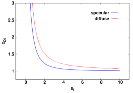
Figure 1: Dependence of the drag coefficient $c_{Di}$ on the molecular speed ratio $s_{i}$ for the cases of specular and diffuse reflection (see text).

For the collision parameter, we can write

$$\gamma_{i}=n_{i}~{}\frac{m_{i}}{m}~{}A~{},$$ (4)

where $n_{i}$ is the concentration of the interstellar neutral atoms of type $i$, and $A$ $=$ $\pi{R}^{2}$ is the geometrical cross section of the spherical dust grain of radius $R$ and mass $m$. For $s_{i}$ $\ll$ 1, or, more precisely, if $s_{i}^{2}$ is negligible in comparison with $s_{i}$ is possible to show that

$$c_{Di}(s_{i})=\frac{8}{3}\frac{1}{\sqrt{\pi}}\frac{1}{s_{i}}+\left(1-\delta_{i}\right)\left(\frac{T_{d}}{T_{i}}\right)^{1/2}\frac{\sqrt{\pi}}{3s_{i}}~{}.$$ (5)

As a consequence acceleration of the dust particle is (Baines, Williams & Asebiomo, 1965)

$$\frac{d\vec{v}}{dt} = -\sum_{i}\frac{8}{3}\frac{1}{\sqrt{\pi}}\left[1+\left(1-\delta_{i}\right)\left(\frac{T_{d}}{T_{i}}\right)^{1/2}\frac{\pi}{8}\right]~{}\gamma_{i}$$ (6)

$$\times~{}\sqrt{\frac{2kT_{i}}{m_{i}}}~{}\left(\vec{v}-\vec{v}_{F}\right)~{}.$$

Hence, for $s_{i}$ $\ll$ 1 acceleration depends linearly on the relative velocity vector $\vec{v}-\vec{v}_{F}$. The case $s_{i}$ $\ll$ 1 will be no further discussed in this parer.

We want to find the influence of an interstellar gas flow on the secular evolution of a particle’s orbit. We assume that the dust particle is under the action of the gravitation of the Sun and the flow of a neutral gas. Hence, we have the equation of motion

$$\frac{d\vec{v}}{dt}=-~{}\frac{\mu}{r^{3}}~{}\vec{r}~{}-~{}\sum_{i}c_{Di}~{}\gamma_{i}~{}|\vec{v}-\vec{v}_{F}|~{}\left(\vec{v}-\vec{v}_{F}\right)~{},$$ (7)

where $\mu$ $=$ $GM_{\odot}$, $G$ is the gravitational constant, $M_{\odot}$ is the mass of the Sun, $\vec{r}$ is the position vector of the dust particle with respect to the Sun, and $r$ $=$ $|\vec{r}|$.

We will assume that the speed of the interstellar gas flow is much greater than the speed of the dust grain in the stationary frame associated with the Sun:

$$|\vec{v}|=v\ll|\vec{v}_{F}|=v_{F}~{}.$$ (8)

Therefore, we can write

$$U = |\vec{v}-\vec{v}_{F}|=\sqrt{v^{2}+v_{F}^{2}-2~{}\vec{v}\cdot\vec{v}_{F}}$$ (9)

$$\approx v_{F}~{}\left(1-\frac{\vec{v}\cdot\vec{v}_{F}}{v_{F}^{2}}\right)~{}.$$

In the above equation, we have considered only the terms to the first order in $v/v_{F}$. Using this approximation, we can also approximate changes in the drag coefficient $c_{Di}$ in Eq. (2). We have

$$c_{Di}(s_{i}) \approx c_{Di}(s_{0i})+\left(\frac{dc_{Di}}{ds_{i}}\right)_{s_{i}=s_{0i}}(s_{i}-s_{0i})$$ (10)

$$\equiv c_{Di}(s_{0i})+\left(\frac{dc_{Di}}{ds_{i}}\right)_{s_{i}=s_{0i}}\sqrt{\frac{m_{i}}{2kT_{i}}}~{}(U-v_{F})$$

$$\approx c_{0i}-k_{i}~{}\frac{\vec{v}\cdot\vec{v}_{F}}{v_{F}}~{},$$

where

$$s_{0i} \equiv \sqrt{\frac{m_{i}}{2kT_{i}}}~{}v_{F}~{},$$

$$c_{0i} \equiv c_{Di}(s_{0i})~{},$$

$$k_{i} \equiv \left(\frac{dc_{Di}}{ds_{i}}\right)_{s_{i}=s_{0i}}~{}\sqrt{\frac{m_{i}}{2kT_{i}}}~{}.$$ (11)

We can rewrite Eq. (7) using these two approximations into the following form

$$\frac{d\vec{v}}{dt} = -~{}\frac{\mu}{r^{3}}\vec{r}~{}-~{}\sum_{i}c_{0i}~{}\gamma_{i}~{}v_{F}^{2}\biggl{[}\frac{\vec{v}}{v_{F}}-\frac{\vec{v_{F}}}{v_{F}}$$ (12)

$$+~{}\left(1+\frac{k_{i}}{c_{0i}}v_{F}\right)\frac{\vec{v}\cdot\vec{v}_{F}}{v_{F}^{2}}\frac{\vec{v_{F}}}{v_{F}}\biggr{]}~{}.$$

This equation allows using the perturbation theory of celestial mechanics to compute the secular evolution of the dust particle under the action of the interstellar gas flow. For the secular time derivatives of the Keplerian orbital elements caused by the interstellar gas flow, we finally obtain (see Appendix A)

$$\left\langle\frac{da}{dt}\right\rangle = -\sum_{i}2~{}a~{}c_{0i}~{}\gamma_{i}~{}v_{F}^{2}~{}\sqrt{\frac{p}{\mu}}~{}\sigma~{}\Biggl{\{}1+\frac{1}{v_{F}^{2}}$$ (13)

$$\times~{}\left(1+\frac{k_{i}}{c_{0i}}v_{F}\right)\Biggl{[}I^{2}-(I^{2}-S^{2})$$

$$\times~{}\frac{1-\sqrt{1-e^{2}}}{e^{2}}\Biggr{]}\Biggr{\}}~{},$$

$$\left\langle\frac{de}{dt}\right\rangle = \sum_{i}c_{0i}~{}\gamma_{i}~{}v_{F}~{}\sqrt{\frac{p}{\mu}}~{}\Biggl{[}\frac{3I}{2}+\frac{\sigma(I^{2}-S^{2})(1-e^{2})}{v_{F}e^{3}}$$ (14)

$$\times~{}\left(1+\frac{k_{i}}{c_{0i}}v_{F}\right)\left(1-\frac{e^{2}}{2}-\sqrt{1-e^{2}}\right)\Biggr{]}~{},$$

$$\left\langle\frac{d\omega}{dt}\right\rangle = \sum_{i}\frac{c_{0i}~{}\gamma_{i}~{}v_{F}}{2}~{}\sqrt{\frac{p}{\mu}}~{}\Biggl{\{}-~{}\frac{3S}{e}$$ (15)

$$+~{}\frac{\sigma SI}{v_{F}e^{4}}\left(1+\frac{k_{i}}{c_{0i}}v_{F}\right)$$

$$\times~{}\biggl{[}e^{4}-6e^{2}+4-4(1-e^{2})^{3/2}\biggr{]}$$

$$+~{}C~{}\frac{\cos i}{\sin i}~{}\biggl{[}\frac{3e\sin\omega}{1-e^{2}}-\frac{\sigma}{v_{F}}\left(1+\frac{k_{i}}{c_{0i}}v_{F}\right)$$

$$\times~{}(S\cos\omega-I\sin\omega)\biggr{]}\Biggr{\}}~{},$$

$$\left\langle\frac{d\Omega}{dt}\right\rangle = \sum_{i}\frac{c_{0i}~{}\gamma_{i}~{}v_{F}~{}C}{2~{}\sin i}~{}\sqrt{\frac{p}{\mu}}~{}\Biggl{[}-~{}\frac{3e\sin\omega}{1-e^{2}}$$ (16)

$$+~{}\frac{\sigma}{v_{F}}\left(1+\frac{k_{i}}{c_{0i}}v_{F}\right)(S\cos\omega-I\sin\omega)\Biggr{]}~{},$$

$$\left\langle\frac{di}{dt}\right\rangle = -\sum_{i}\frac{c_{0i}~{}\gamma_{i}~{}v_{F}~{}C}{2}~{}\sqrt{\frac{p}{\mu}}~{}\Biggl{[}\frac{3e\cos\omega}{1-e^{2}}$$ (17)

$$+~{}\frac{\sigma}{v_{F}}\left(1+\frac{k_{i}}{c_{0i}}v_{F}\right)(S\sin\omega+I\cos\omega)\Biggr{]}~{},$$

where $p$ $=$ $a(1-e^{2})$,

$$\sigma=\frac{\sqrt{\mu/p}}{v_{F}}~{},$$ (18)

and the quantities

$$S = (\cos\Omega~{}\cos\omega-\sin\Omega~{}\sin\omega~{}\cos i)~{}v_{FX}$$

$$+~{}(\sin\Omega~{}\cos\omega+\cos\Omega~{}\sin\omega~{}\cos i)~{}v_{FY}$$

$$+~{}\sin\omega~{}\sin i~{}v_{FZ}~{},$$

$$I = (-\cos\Omega~{}\sin\omega-\sin\Omega~{}\cos\omega~{}\cos i)~{}v_{FX}$$

$$+~{}(-\sin\Omega~{}\sin\omega+\cos\Omega~{}\cos\omega~{}\cos i)~{}v_{FY}$$

$$+~{}\cos\omega~{}\sin i~{}v_{FZ}~{},$$

$$C = \sin\Omega~{}\sin i~{}v_{FX}-\cos\Omega~{}\sin i~{}v_{FY}$$ (19)

$$+~{}\cos i~{}v_{FZ}~{},$$

are the values of $A$ $=$ $\vec{v}_{F}\cdot\vec{e}_{R}$, $B$ $=$ $\vec{v}_{F}\cdot\vec{e}_{T}$, and $C$ $=$ $\vec{v}_{F}\cdot\vec{e}_{N}$, at the perihelion of the particle’s orbit ($f$ $=$ 0), respectively. For a complete solution of this system of equations for $\sigma$ $=$ 0 (constant force), we refer the reader to Pástor (2012).

3 Discussion

$C$ $=$ 0 for the special case when the velocity of the interstellar gas, $\vec{v}_{F}$, lies in the orbital plane of the particle. In this planar case, we find that the inclination and the longitude of the ascending node are constant.

Eq. (15) implies that the argument of the perihelion is constant in the planar case ($C$ $\equiv$ 0) and if the orbit’s orientation is characterised by $S$ $=$ 0.

The dependence of the drag coefficients on the relative speed of the dust particle with respect to the interstellar gas is demonstrated by the presence of terms multiplied by $k_{i}$ in Eqs. (13)–(17). It is convenient to define a new function

$$g_{i}=1+\frac{k_{i}}{c_{0i}}v_{F}~{}.$$ (20)

In order to find the influence of a non-constant drag coefficients on the evolution of the particle’s orbit we will analyse the properties of this function. We can write, see Eqs. (2),

$$g_{i} = 1+\left(\frac{dc_{Di}}{ds_{i}}\right)_{s_{i}=s_{0i}}\frac{s_{0i}}{c_{0i}}$$ (21)

$$= \frac{1}{c_{0i}}\biggl{[}\frac{1}{\sqrt{\pi}}\left(\frac{1}{s_{0i}}-\frac{3}{2s_{0i}^{3}}\right)e^{-s_{0i}^{2}}$$

$$+~{}\left(1-\frac{1}{s_{0i}^{2}}+\frac{3}{4s_{0i}^{4}}\right)\mbox{erf}(s_{0i})\biggr{]}~{}.$$

The graph of $g_{i}$ for the case of specular ($\delta_{i}$ $=$ 1) and diffuse ($\delta_{i}$ $=$ 0, $T_{d}$ $=$ $T_{i}$) reflection is depicted in Fig. 2.

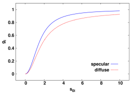
Figure 2: Dependence of $g_{i}$ on $s_{0i}$ for the case of specular and diffuse reflection.

The function $g_{i}$ is an increasing function of $s_{0i}$ for $s_{0i}$ $\in$ (0, $\infty$) (see Appendix B). $\lim_{s_{0i}\to 0}g_{i}$ $=$ 0 and $\lim_{s_{0i}\to\infty}g_{i}$ $=$ 1. Hence, we can conclude that $g_{i}$ $\in$ [0, 1].

Eq. (13) can be rewritten in the following form.

$$\left\langle\frac{da}{dt}\right\rangle = -\sum_{i}2~{}a~{}c_{0i}~{}\gamma_{i}~{}v_{F}^{2}~{}\sqrt{\frac{p}{\mu}}~{}\sigma~{}\Biggl{[}1+\frac{1}{v_{F}^{2}}$$ (22)

$$\times~{}\left(1+\frac{k_{i}}{c_{0i}}v_{F}\right)\frac{1-\sqrt{1-e^{2}}}{e^{2}}$$

$$\times~{}\left(I^{2}\sqrt{1-e^{2}}+S^{2}\right)\Biggr{]}~{}.$$

Thus, the semimajor axis is a decreasing function of time. This result, when $k_{i}$ $=$ 0, was already obtained in Pástor et al. (2011), and generalised to the case $k_{i}$ $\neq$ 0 in Belyaev & Rafikov (2010). If we use the properties of $g_{i}$, then from Eq. (22) we can conclude that the dependence of the drag coefficients on the relative speed of the dust particle has a tendency to reduce the decrease of the semimajor axis caused by the interstellar gas flow.

In order to find the orbit orientation with minimal and maximal decrease of the semimajor axis, we will analyse the second term in the square brace in Eq. (22),

$$\phi=\frac{1}{v_{F}^{2}}\left(1+\frac{k_{i}}{c_{0i}}v_{F}\right)\frac{1-\sqrt{1-e^{2}}}{e^{2}}\left(I^{2}\sqrt{1-e^{2}}+S^{2}\right)~{}.$$ (23)

Because the terms multiplied by $S^{2}$ and $I^{2}$ are both positive, we obtain a minimal value of $\phi$ when $S$ $=$ 0 and $I$ $=$ 0. Therefore, if the orbital plane is perpendicular to the interstellar gas flow velocity vector, then the decrease of the semimajor axis is minimal (Fig. 3).

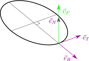
Figure 3: An orbit orientation with minimal decrease of the semimajor axis.

From Eq. (22), we obtain for $S$ $=$ 0 and $I$ $=$ 0,

$$\left\langle\frac{da}{dt}\right\rangle_{min}=-\sum_{i}2~{}a~{}c_{0i}~{}\gamma_{i}~{}v_{F}~{}.$$ (24)

The value of the minimal decrease is proportional to the semimajor axis and independent of the orbit eccentricity.

Because the terms multiplied by $S^{2}$ and $I^{2}$ are both positive, we obtain a maximal value of $\phi$ when $C$ $=$ 0. If $C$ $=$ 0, then $S^{2}$ $+$ $I^{2}$ $=$ $v_{F}^{2}$. Using this, the value of $\phi$ can be written as

$$\phi = \frac{1}{v_{F}^{2}}\left(1+\frac{k_{i}}{c_{0i}}v_{F}\right)\frac{1-\sqrt{1-e^{2}}}{e^{2}}$$ (25)

$$\times~{}\left[v_{F}^{2}\sqrt{1-e^{2}}+S^{2}(1-\sqrt{1-e^{2}})\right]~{}.$$

Here, $v_{F}^{2}$ is constant. Therefore, we obtain the maximal value of $\phi$ for an orbit orientation characterized by $S^{2}$ $=$ $v_{F}^{2}$. Hence, the maximal value of $\phi$ is

$$\phi=\left(1+\frac{k_{i}}{c_{0i}}v_{F}\right)\frac{1-\sqrt{1-e^{2}}}{e^{2}}=\left(1+\frac{k_{i}}{c_{0i}}v_{F}\right)h(e)~{}.$$ (26)

Therefore, if the interstellar gas flow velocity vector is parallel to the line of apsides, then the decrease of the semimajor axis is maximal (Fig. 4).

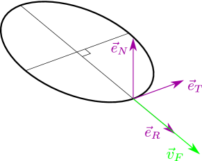
Figure 4: An orbit orientation with maximal decrease of the semimajor axis.

For a given orbit, the maximal decrease of the semimajor axis is

$$\left\langle\frac{da}{dt}\right\rangle_{max} = -\sum_{i}2~{}a~{}c_{0i}~{}\gamma_{i}~{}v_{F}~{}\Biggl{[}1+\left(1+\frac{k_{i}}{c_{0i}}v_{F}\right)$$ (27)

$$\times~{}\frac{1-\sqrt{1-e^{2}}}{e^{2}}\Biggl{]}~{}.$$

The function $h(e)$ defined in Eq. (26) is an increasing function of the eccentricity (see Appendix C). Therefore, the decrease of the semimajor axis is maximal for $e$ $=$ 1.

For the secular time derivatives of $S$, $I$, and $C$, we obtain from Eq. (2) and Eqs. (15), (16) and (17),

$$\left\langle\frac{dS}{dt}\right\rangle = \sum_{i}\frac{c_{0i}~{}\gamma_{i}~{}v_{F}~{}S}{2}~{}\sqrt{\frac{p}{\mu}}~{}\Biggl{\{}-~{}\frac{3I}{e}$$ (28)

$$-~{}\frac{\sigma}{v_{F}}\left(1+\frac{k_{i}}{c_{0i}}v_{F}\right)\biggl{[}C^{2}-\frac{I^{2}}{e^{4}}\biggl{(}e^{4}-6e^{2}$$

$$+~{}4-4(1-e^{2})^{3/2}\biggr{)}\biggr{]}\Biggr{\}}~{},$$

$$\left\langle\frac{dI}{dt}\right\rangle = \sum_{i}\frac{c_{0i}~{}\gamma_{i}~{}v_{F}}{2}~{}\sqrt{\frac{p}{\mu}}~{}\Biggl{\{}-~{}\frac{3eC^{2}}{1-e^{2}}+\frac{3S^{2}}{e}$$ (29)

$$-~{}\frac{\sigma I}{v_{F}}\left(1+\frac{k_{i}}{c_{0i}}v_{F}\right)\biggl{[}C^{2}+\frac{S^{2}}{e^{4}}\biggl{(}e^{4}-6e^{2}$$

$$+~{}4-4(1-e^{2})^{3/2}\biggr{)}\biggr{]}\Biggr{\}}~{},$$

$$\left\langle\frac{dC}{dt}\right\rangle = \sum_{i}\frac{c_{0i}~{}\gamma_{i}~{}v_{F}~{}C}{2}~{}\sqrt{\frac{p}{\mu}}~{}\Biggl{[}\frac{3eI}{1-e^{2}}$$ (30)

$$+~{}\frac{\sigma}{v_{F}}\left(1+\frac{k_{i}}{c_{0i}}v_{F}\right)(S^{2}+I^{2})\Biggr{]}~{}.$$

Eqs. (28)–(30) are not independent, because $S\langle dS/dt\rangle$ $+$ $I\langle dI/dt\rangle$ $+$ $C\langle dC/dt\rangle$ $=$ 0 always holds. Eqs. (28)–(30), together with Eqs. (13) and (14), represent the system of equations that determines the evolution of the particle’s orbit in space with respect to the interstellar gas velocity vector. All orbits that are created from rotations of one orbit around the line aligned with the interstellar gas velocity vector and going through the centre of gravity will undergo the same evolution determined by this system of equations. If $\sigma$ is small and $I$ and $e$ are not close to zero, we can use the following approximate solution for $S$, $I$, and $C$ (see Pástor et al. 2011).

$$S\approx\frac{U}{e}~{},$$ (31)

$$C\approx\frac{V}{\sqrt{1-e^{2}}}$$ (32)

and

$$|I|\approx\sqrt{v_{F}^{2}-\frac{U^{2}}{e^{2}}-\frac{V^{2}}{1-e^{2}}}~{},$$ (33)

where $U$ and $V$ are some constants.

Now, we want to find the evolution of the orbit position in the planar case. For this purpose we can use Eq. (29), which determines the time evolution of $I$. Eq. (29) implies, for the planar case ($C$ $\equiv$ 0),

$$\left\langle\frac{dI}{dt}\right\rangle = \sum_{i}\frac{c_{0i}~{}\gamma_{i}~{}v_{F}~{}S^{2}}{2}~{}\sqrt{\frac{p}{\mu}}~{}\Biggl{[}\frac{3}{e}-\frac{\sigma I}{v_{F}}$$ (34)

$$\times~{}\left(1+\frac{k_{i}}{c_{0i}}v_{F}\right)b(e)\Biggr{]}~{}.$$

Here,

$$b(e)=\frac{e^{4}-6e^{2}+4-4(1-e^{2})^{3/2}}{e^{4}}~{}.$$ (35)

The function $b(e)$ is a decreasing function of eccentricity for $e$ $\in$ (0, 1] (see Pástor et al. 2011, Appendix B). The function $b(e)$ attains values from $\lim_{e\to 0}b(e)$ $=$ $-$ 0.5 to $b(1)$ $=$ $-$ 1, for $e$ $\in$ (0, 1]. Since we have assumed that $v$ $\ll$ $v_{F}$, see Eq. (8), we have for the maximal speed of the dust particle in the perihelion of the particle’s orbit, see Eq. (52),

$$v_{max}=\sqrt{\frac{\mu}{p}}~{}(1+e)\ll v_{F}~{}.$$ (36)

Hence

$$\sigma=\frac{\sqrt{\mu/p}}{v_{F}}\leq\frac{\sqrt{\mu/p}}{v_{F}}~{}(1+e)\ll 1~{}.$$ (37)

For $I$ $>$ 0, one always has $\langle dI/dt\rangle$ $>$ 0. Therefore, we will assume that $I$ $<$ 0. For negative $I$, we can write

$$\frac{\sigma I}{v_{F}}\left(1+\frac{k_{i}}{c_{0i}}v_{F}\right)b(e)\leq\frac{\sigma I}{v_{F}}~{}b(e)\leq-\sigma~{}b(e)\leq\sigma<\frac{3}{e}~{},$$ (38)

as $1+k_{i}~{}v_{F}/c_{0i}$ $\leq$ 1, see the discussion after Eq. (21), $-$ $I$ $\leq$ $v_{F}$, $b(e)$ $\in$ ($-$ 0.5, $-$ 1], and $\sigma$ $\ll$ 1. If we rearrange (38), then we come to the conclusion that $\langle dI/dt\rangle$ $>$ 0 also for $I$ $<$ 0. Therefore, in the planar case, $I$ is always an increasing function of time. Thus, in the planar case the orbit rotates into position with a maximal value of $I$. In this position, the line of apsides is perpendicular to the interstellar gas flow velocity vector.

4 Numerical results

4.1 Accelerations influencing the dynamics of dust grains inside the heliosphere

For a correct description of the motion of micron-sized dust particles inside the heliosphere, solar electromagnetic radiation and the solar wind must also be considered.

4.1.1 Electromagnetic radiation

The acceleration of a dust particle with spherically distributed mass caused by electromagnetic radiation to the first order in $v/c$ is given by the PR effect (Poynting, 1903; Robertson, 1937; Wyatt & Whipple, 1950; Burns, Lamy & Soter, 1979; Klačka, 2004; Klačka et al., 2012b):

$$\frac{d\vec{v}}{dt}=\beta~{}\frac{\mu}{r^{2}}\left[\left(1-\frac{\vec{v}\cdot\vec{e}_{R}}{c}\right)\vec{e}_{R}-\frac{\vec{v}}{c}\right]~{},$$ (39)

where $\vec{e}_{R}$ $=$ $\vec{r}/r$ and $c$ is the speed of light in vacuum. The parameter $\beta$ is defined as the ratio of the electromagnetic radiation pressure force and the gravitational force between the Sun and the particle at rest with respect to the Sun

$$\beta=\frac{3~{}L_{\odot}~{}\bar{Q}^{\prime}_{pr}}{16~{}\pi~{}c~{}\mu~{}R~{}\varrho}~{}.$$ (40)

Here, $L_{\odot}$ is the solar luminosity, $L_{\odot}$ $=$ 3.842 $\times$ 10²⁶ W (Bahcall, 2002), $\bar{Q}^{\prime}_{pr}$ is the dimensionless efficiency factor for radiation pressure integrated over the solar spectrum and calculated for the radial direction ($\bar{Q}^{\prime}_{pr}$ $=$ 1 for a perfectly absorbing sphere), and $\varrho$ is the mass density of the particle.

4.1.2 Radial solar wind

Acceleration caused by the radial solar wind to the first order of $v/c$ and the first order of $v/u$ is given by (Klačka et al., 2012a, Eq. 37):

$$\frac{d\vec{v}}{dt}=\frac{\eta}{\bar{Q}^{\prime}_{pr}}~{}\beta~{}\frac{u}{c}~{}\frac{\mu}{r^{2}}\left[\left(1-\frac{\vec{v}\cdot\vec{e}_{R}}{u}\right)\vec{e}_{R}-\frac{\vec{v}}{u}\right]~{}.$$ (41)

Here, $u$ is the speed of the solar wind with respect to the Sun, $u$ $=$ 450 km/s. $\eta$ is the ratio of solar wind energy to electromagnetic solar energy, both radiated per unit of time

$$\eta=\frac{4~{}\pi~{}r^{2}~{}u}{L_{\odot}}~{}\sum_{i=1}^{N}n_{sw~{}i}~{}m_{sw~{}i}~{}c^{2}~{},$$ (42)

where $m_{sw~{}i}$ and $n_{sw~{}i}$, $i$ $=$ 1 to $N$, are the masses and concentrations of the solar wind particles at a distance $r$ from the Sun. $\eta$ $=$ 0.38 for the Sun (Klačka et al., 2012a).

4.1.3 Acceleration caused by solar gravity, solar radiation, and interstellar gas flow

In order to find the acceleration of the dust particle inside the heliosphere, we can sum the gravitational acceleration from the Sun, the acceleration from the PR effect Eq. (39), the acceleration from the solar wind Eq. (41), and the acceleration from the interstellar gas Eq. (1).

$$\frac{d\vec{v}}{dt} = -~{}\frac{\mu}{r^{2}}~{}\left(1-\beta\right)~{}\vec{e}_{R}$$ (43)

$$-~{}\beta~{}\frac{\mu}{r^{2}}\left(1+\frac{\eta}{\bar{Q}^{\prime}_{pr}}\right)\left(\frac{\vec{v}\cdot\vec{e}_{R}}{c}~{}\vec{e}_{R}+\frac{\vec{v}}{c}\right)$$

$$-~{}\sum_{i}c_{Di}~{}\gamma_{i}~{}|\vec{v}-\vec{v}_{F}|~{}\left(\vec{v}-\vec{v}_{F}\right)$$

Here, it is assumed that $(\eta/\bar{Q}^{\prime}_{pr})(u/c)$ $\ll$ 1.

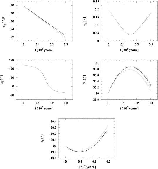
Figure 5: A comparison of the solution of the equation of motion (solid lines) with the solution of the system of differential equations constituted by the secular time derivatives of the Keplerian orbital elements (dashed lines). The solutions with variable (black lines) and constant (grey lines) drag coefficients are compared.

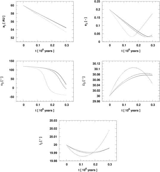
Figure 6: Orbital evolution under the action of the PR effect, radial solar wind, and interstellar gas flow, obtained from numerical solution of Eq. (43) (black line) and from numerical solution of the system of differential equations Eqs. (44)–(48) (grey line). We used interstellar gas with three different temperatures $T_{1}$ $=$ 500 K (solid line), $T_{1}$ $=$ 5000 K (dashed line) and $T_{1}$ $=$ 50000 K (dotted line).

4.2 Comparison of the solution of the equation of motion with the solution of the system of equations constituted by the secular time derivatives of the Keplerian orbital elements

We want to compare the solution obtained from Eq. (43) with the solution of the system of equations constituted by the secular time derivatives of the Keplerian orbital elements. To do this, we need to add to the right hand sides of Eqs. (13)–(17) also the secular time derivatives of the Keplerian orbital elements caused by the PR effect and the radial solar wind. Therefore, we solved the following system of equations (Wyatt & Whipple, 1950; Klačka et al., 2012a)

$$\left\langle\frac{da_{\beta}}{dt}\right\rangle = -~{}\beta~{}\frac{\mu}{c}~{}\left(1+\frac{\eta}{\bar{Q}^{\prime}_{pr}}\right)~{}\frac{2+3e_{\beta}^{2}}{a_{\beta}~{}(1-e_{\beta}^{2})^{3/2}}$$ (44)

$$-~{}\sum_{i}2~{}a_{\beta}~{}c_{0i}~{}\gamma_{i}~{}v_{F}^{2}~{}\sqrt{\frac{p_{\beta}}{\mu\left(1-\beta\right)}}~{}\sigma_{\beta}$$

$$\times~{}\Biggl{\{}1+\frac{1}{v_{F}^{2}}\left(1+\frac{k_{i}}{c_{0i}}v_{F}\right)\Biggl{[}I_{\beta}^{2}-(I_{\beta}^{2}-S_{\beta}^{2})$$

$$\times~{}\frac{1-\sqrt{1-e_{\beta}^{2}}}{e_{\beta}^{2}}\Biggr{]}\Biggr{\}}~{},$$

$$\left\langle\frac{de_{\beta}}{dt}\right\rangle = -~{}\beta~{}\frac{\mu}{c}~{}\left(1+\frac{\eta}{\bar{Q}^{\prime}_{pr}}\right)~{}\frac{5~{}e_{\beta}}{2~{}a_{\beta}^{2}~{}(1-e_{\beta}^{2})^{1/2}}$$ (45)

$$+~{}\sum_{i}c_{0i}~{}\gamma_{i}~{}v_{F}~{}\sqrt{\frac{p_{\beta}}{\mu\left(1-\beta\right)}}$$

$$\times~{}\Biggl{[}\frac{3I_{\beta}}{2}+\frac{\sigma_{\beta}(I_{\beta}^{2}-S_{\beta}^{2})(1-e_{\beta}^{2})}{v_{F}e_{\beta}^{3}}\left(1+\frac{k_{i}}{c_{0i}}v_{F}\right)$$

$$\times~{}\left(1-\frac{e_{\beta}^{2}}{2}-\sqrt{1-e_{\beta}^{2}}\right)\Biggr{]}~{},$$

$$\left\langle\frac{d\omega_{\beta}}{dt}\right\rangle = \sum_{i}\frac{c_{0i}~{}\gamma_{i}~{}v_{F}}{2}~{}\sqrt{\frac{p_{\beta}}{\mu\left(1-\beta\right)}}~{}\Biggl{\{}-~{}\frac{3S_{\beta}}{e_{\beta}}$$ (46)

$$+~{}\frac{\sigma_{\beta}S_{\beta}I_{\beta}}{v_{F}e_{\beta}^{4}}\left(1+\frac{k_{i}}{c_{0i}}v_{F}\right)$$

$$\times~{}\biggl{[}e_{\beta}^{4}-6e_{\beta}^{2}+4-4(1-e_{\beta}^{2})^{3/2}\biggr{]}$$

$$+~{}C_{\beta}~{}\frac{\cos i_{\beta}}{\sin i_{\beta}}~{}\biggl{[}\frac{3e_{\beta}\sin\omega_{\beta}}{1-e_{\beta}^{2}}-\frac{\sigma_{\beta}}{v_{F}}\left(1+\frac{k_{i}}{c_{0i}}v_{F}\right)$$

$$\times~{}(S_{\beta}\cos\omega_{\beta}-I_{\beta}\sin\omega_{\beta})\biggr{]}\Biggr{\}}~{},$$

$$\left\langle\frac{d\Omega_{\beta}}{dt}\right\rangle = \sum_{i}\frac{c_{0i}~{}\gamma_{i}~{}v_{F}~{}C_{\beta}}{2~{}\sin i_{\beta}}~{}\sqrt{\frac{p_{\beta}}{\mu\left(1-\beta\right)}}$$ (47)

$$\times~{}\Biggl{[}-~{}\frac{3e_{\beta}\sin\omega_{\beta}}{1-e_{\beta}^{2}}+\frac{\sigma_{\beta}}{v_{F}}\left(1+\frac{k_{i}}{c_{0i}}v_{F}\right)$$

$$\times~{}(S_{\beta}\cos\omega_{\beta}-I_{\beta}\sin\omega_{\beta})\Biggr{]}~{},$$

$$\left\langle\frac{di_{\beta}}{dt}\right\rangle = -\sum_{i}\frac{c_{0i}~{}\gamma_{i}~{}v_{F}~{}C_{\beta}}{2}~{}\sqrt{\frac{p_{\beta}}{\mu\left(1-\beta\right)}}$$ (48)

$$\times~{}\Biggl{[}\frac{3e_{\beta}\cos\omega_{\beta}}{1-e_{\beta}^{2}}+\frac{\sigma_{\beta}}{v_{F}}\left(1+\frac{k_{i}}{c_{0i}}v_{F}\right)$$

$$\times~{}(S_{\beta}\sin\omega_{\beta}+I_{\beta}\cos\omega_{\beta})\Biggr{]}$$

As the central acceleration, we used the Keplerian acceleration given by the first term in Eq. (43), namely $-\mu(1-\beta)\vec{e}_{R}/r^{2}$. This is denoted by the subscript $\beta$ in Eqs. (44)–(48). In the interstellar gas flow, we have taken into account the primary and secondary populations of neutral hydrogen atoms and neutral helium atoms. The primary population of neutral hydrogen atoms and neutral helium atoms represent the original atoms of the interstellar gas flow which penetrate into the heliosphere. The secondary population of neutral hydrogen atoms are the former protons from the interstellar gas flow that acquired electrons from interstellar H^∘ between the bow shock and the heliopause (Frisch et al., 2009; Alouani-Bibi et al., 2011). We adopted the following parameters for these components in the interstellar gas flow. $n_{1}$ $=$ 0.059 cm^-3 and $T_{1}$ $=$ 6100 K for the primary population of neutral hydrogen (Frisch et al., 2009), $n_{2}$ $=$ 0.059 cm^-3 and $T_{2}$ $=$ 16500 K for the secondary population of neutral hydrogen (Frisch et al., 2009) and finally $n_{3}$ $=$ 0.015 cm^-3 and $T_{3}$ $=$ 6300 K for the neutral helium (Lallement et al., 2005). We have assumed that the interstellar gas velocity vector is equal for all components and identical to the velocity vector of the neutral helium entering the Solar system. The neutral helium enter the Solar system with a speed of about $v_{F}$ $=$ 26.3 km s^-1 (Lallement et al., 2005), and arrive from the direction of $\lambda_{ecl}$ $=$ 254.7^∘ (heliocentric ecliptic longitude) and $\beta_{ecl}$ $=$ 5.2^∘ (heliocentric ecliptic latitude; Lallement et al. 2005). Thus, the components of the velocity in the ecliptic coordinates with the $x$-axis aligned towards the actual equinox are $\vec{v}_{F}$ $=$ $-$ 26.3 km/s [$\cos(254.7^{\circ})\cos(5.2^{\circ})$, $\sin(254.7^{\circ})\cos(5.2^{\circ})$, $\sin(5.2^{\circ})$]. We want also to demonstrate the influence of a variable drag coefficient on the secular orbital evolution of the dust particle’s orbit. Therefore, we solved Eq. (43) and the system of Eqs. (44)–(48) in two cases. One with variable drag coefficients and one with constant drag coefficients. The variable drag coefficients for Eq. (43) were calculated from Eq. (2). We assumed that the atoms are specularly reflected at the surface of the dust grain ($\delta_{i}$ $=$ 1). As the initial conditions for a dust particle with $R$ $=$ 2 $\mu$m, mass density $\varrho$ $=$ 1 g/cm³, and $\bar{Q}^{\prime}_{pr}$ $=$ 1, we used $a_{in}$ $=$ 60 AU, $e_{in}$ $=$ 0.2, $\omega_{in}$ $=$ 120^∘, $\Omega_{in}$ $=$ 30^∘, and $i_{in}$ $=$ 20^∘. The initial true anomaly of the dust particle was $f_{in}$ $=$ 180^∘ for Eq. (43). The results are depicted in Fig. 5. The solid lines are used for the solution of Eq. (43) and the dashed lines are used for the solution of Eqs. (44)–(48). The black lines are used for the variable drag coefficients and the grey lines are used for constant drag coefficients. The solution of Eqs. (44)–(48) with constant drag coefficients can be obtained by putting $k_{i}$ $=$ 0 in Eqs. (44)–(48). Fig. 5 shows that the solution of the equation of motion (Eq. 43) is in good accordance with the solution of the system of equations constituted by the secular time derivatives of the Keplerian orbital elements Eqs. (44)–(48), for both variable and constant drag coefficients. The semimajor axis decreases faster for the constant drag coefficients. This is in accordance with the properties of the function $g_{i}$ (see the discussion after Eq. 21 and Eq. 22). The numerical solutions depicted in Fig. 5 represent the cases for which Eq. (8) holds. In these cases, the influence of the variable drag coefficient in the acceleration caused by the interstellar gas flow on the orbital evolution of the dust particle is not large and in some cases can be neglected (as we can see in Fig. 5).

4.3 Validity of the linear approximation at various Mach numbers

Fig. 6 compares solutions of Eq. (43) (black line) with solutions of Eqs. (44)–(48) (grey line). The variability of the drag coefficient in Eq. (43) was given by Eq. (2). We used an artificial interstellar gas flow which consists only of neutral hydrogen atoms with concentration $n_{1}$ $=$ 0.1 cm^-3. The hydrogen gas velocity vector with respect to the Sun was $\vec{v}_{F}$ $=$ (10 km s^-1, 25 km s^-1, 5 km s^-1). In order to visualise the influence of the molecular speed ratio (Mach number) on the orbital evolutions, we used three different temperatures: $T_{1}$ $=$ 500 K (solid line), $T_{1}$ $=$ 5000 K (dashed line) and $T_{1}$ $=$ 50000 K (dotted line). These parameters correspond to Mach numbers (the first equation in Eqs. 2) $s_{01}$ $=$ 9.5, $s_{01}$ $=$ 3.0, and $s_{01}$ $=$ 1.0. Condition $s_{01}$ $\ll$ 1 does not hold for none of these values. Therefore, derivation of Eqs. (44)–(48) using the acceleration caused by the interstellar gas flow described by Eq. (1) is correct (condition for validity of Eq. 6, $s_{01}$ $\ll$ 1, is not fulfilled). As the initial conditions for a dust particle with $R$ $=$ 2 $\mu$m, $\varrho$ $=$ 1 g/cm³ and $\bar{Q}^{\prime}_{pr}$ $=$ 1, we used $a_{in}$ $=$ 60 AU, $e_{in}$ $=$ 0.2, $\omega_{in}$ $=$ 120^∘, $\Omega_{in}$ $=$ 30^∘, and $i_{in}$ $=$ 20^∘. The initial true anomaly of the dust particle was $f_{in}$ $=$ 180^∘ for Eq. (43). Fig. 6 shows that the orbital evolution under the action of the PR effect, radial solar wind, and interstellar gas flow, is well described by the solution of Eqs. (44)–(48) also for the various values of Mach numbers. The fact that evolution of the dust particle under the action of an interstellar gas flow with a larger temperature is faster is caused by proportionality of the secular time derivatives to $c_{01}$. $c_{01}$ is larger for an interstellar gas flow with a larger temperature (see the first and the second equation in Eqs. (2) and Fig. 1 or Appendix B).

5 Conclusion

We have investigated the orbital evolution of a spherical dust grain under the action of an interstellar gas flow. The acceleration of the dust particle caused by the interstellar gas flow depends on a drag coefficient which is a well determined function of the relative speed of the dust particle with respect to the interstellar gas (Baines, Williams & Asebiomo, 1965). We assumed that the acceleration caused by the interstellar gas flow is small compared to the gravitation of a central object, that the speed of the dust particle is small in comparison with the speed of the interstellar gas flow and that molecular speed ratios of the interstellar gas components are not close to zero. Under these assumptions, we derived the secular time derivatives of all Keplerian orbital elements of the dust particle under the action of the acceleration caused by the interstellar gas flow, with linear variability of the drag coefficient taken into account, for arbitrary orientations of the orbit.

If the variability of the drag coefficient is taken into consideration in the acceleration, then the secular decrease of the semimajor axis is slower. The secular decrease of the semimajor axis is slowest for orbit orientations characterised by the perpendicularity of the orbital plane to the interstellar gas velocity vector. The negative secular time derivative of the semimajor axis is in this case independent of the eccentricity of the orbit. The secular decrease of the semimajor axis is for a given orbit fastest in the planar case (when the interstellar gas velocity vector lies in the orbital plane) with the interstellar gas velocity vector parallel to the line of apsides. For such orbits with various eccentricities is the secular decrease of the semimajor axis fastest for a orbit with largest eccentricity.

Regarding the secular evolutions of the eccentricity, the argument of perihelion, the longitude of the ascending node, and the inclination, we found that the variability of the drag coefficient has a tendency to compensate the influence of the terms multiplied by $\sigma$, see Eqs. (14)–(17). The terms multiplied by $\sigma$ originate from the dependence of the acceleration caused by the interstellar gas flow on the velocity of the dust particle with respect to the central object.

If we consider only the influence of the interstellar gas flow on the orbit of the dust particle, then the product of the secular eccentricity and the magnitude of the radial component of $\vec{v}_{F}$ measured in the perihelion is, approximately constant during the orbital evolution. A simple approximative relation also holds between the secular eccentricity and the magnitude of the normal component of $\vec{v}_{F}$ measured at perihelion.

In the special case when the interstellar gas flow velocity lies in the orbital plane of the particle and the particle is under the action of the PR effect, the radial solar wind, and an interstellar gas flow, the orbit approaches the position with maximal value of the magnitude of the transversal component of $\vec{v}_{F}$ measured at perihelion.

We found, by numerically integrating the equation of motion with a variable drag coefficient, that the linear approximation of the dependence of the drag coefficient on the relative speed of the dust particle with respect to the interstellar gas is usable for practically arbitrary (no close to zero) values of the molecular speed ratios (Mach numbers), if the interstellar gas flow speed is much larger than the speed of the dust particle.

Appendix A Derivation of the secular time derivatives of the Keplerian orbital elements

We want to find the secular time derivatives of the Keplerian orbital elements ($a$, semimajor axis; $e$, eccentricity; $\omega$, argument of perihelion; $\Omega$, longitude of the ascending node; $i$, inclination). We will assume that the acceleration caused by the interstellar gas flow can be used as a perturbation to the central acceleration caused by the solar gravity. We use the Gaussian perturbation equations of celestial mechanics (cf., e.g., Murray & Dermott (1999), Danby (1988)). Therefore we need to determine the radial, transversal, and normal components of the acceleration given by the second term in Eq. (12). The orthogonal radial, transversal, and normal unit vectors of the dust particle in a Keplerian orbit are (cf., e.g., Pástor 2009)

$$\vec{e}_{R} = \left(\cos\Omega~{}\cos(f+\omega)-\sin\Omega~{}\sin(f+\omega)~{}\cos i~{},\right.$$ (49)

$$\left.\sin\Omega~{}\cos(f+\omega)+\cos\Omega~{}\sin(f+\omega)~{}\cos i~{},\right.$$

$$\left.\sin(f+\omega)~{}\sin i\right)~{},$$

$$\vec{e}_{T} = \left(-\cos\Omega~{}\sin(f+\omega)-\sin\Omega~{}\cos(f+\omega)~{}\cos i~{},\right.$$ (50)

$$\left.-\sin\Omega~{}\sin(f+\omega)+\cos\Omega~{}\cos(f+\omega)~{}\cos i~{},\right.$$

$$\left.\cos(f+\omega)~{}\sin i\right)~{},$$

$$\vec{e}_{N} = (\sin\Omega~{}\sin i,-\cos\Omega~{}\sin i,~{}\cos i)~{},$$ (51)

where $f$ is the true anomaly. The velocity of the particle in an elliptical orbit can be calculated from

$$\vec{v} = \frac{d\vec{r}}{dt}=\frac{d}{dt}~{}(r\vec{e}_{R})$$ (52)

$$= r~{}\frac{e\sin f}{1+e\cos f}~{}\frac{df}{dt}~{}\vec{e}_{R}+r~{}\vec{e}_{T}~{}\frac{df}{dt}~{},$$

where

$$r=\frac{p}{1+e\cos{f}}$$ (53)

and $p$ $=$ $a(1-e^{2})$. In this calculation, Kepler’s Second Law, $df/dt$ $=$ $\sqrt{\mu p}/r^{2}$, must be used. Now, we can easily verify that

$$(\vec{v}-\vec{v}_{F})\cdot\vec{e}_{R} = v_{F}~{}\sigma~{}e~{}\sin f-\vec{v}_{F}\cdot\vec{e}_{R}$$ (54)

$$= v_{F}~{}\sigma~{}e~{}\sin f-A~{},$$

$$(\vec{v}-\vec{v}_{F})\cdot\vec{e}_{T} = v_{F}~{}\sigma~{}(1+e\cos f)-\vec{v}_{F}\cdot\vec{e}_{T}$$ (55)

$$= v_{F}~{}\sigma~{}(1+e\cos f)-B~{},$$

$$(\vec{v}-\vec{v}_{F})\cdot\vec{e}_{N} = -~{}\vec{v}_{F}\cdot\vec{e}_{N}=-~{}C~{},$$ (56)

where

$$\sigma=\frac{\sqrt{\mu/p}}{v_{F}}~{}.$$ (57)

Using the notation defined in Eqs. (54)–(56) and Eq. (52), we can write

$$\vec{v}\cdot\vec{v}_{F}=\sigma~{}v_{F}[B+e(A\sin f+B\cos f)]~{}.$$ (58)

If we denote the components of the interstellar gas flow velocity vector in the stationary Cartesian frame associated with the Sun as $\vec{v}_{F}$ $=$ $(v_{FX},v_{FY},v_{FZ})$, then we obtain

$$A\sin f+B\cos f = (-\cos\Omega~{}\sin\omega$$ (59)

$$-~{}\sin\Omega~{}\cos\omega~{}\cos i)~{}v_{FX}$$

$$+~{}(-\sin\Omega~{}\sin\omega$$

$$+~{}\cos\Omega~{}\cos\omega~{}\cos i)~{}v_{FY}$$

$$+~{}\cos\omega~{}\sin i~{}v_{FZ}=I~{}.$$

Hence,

$$\vec{v}\cdot\vec{v}_{F}=\sigma~{}v_{F}~{}(B+eI)~{}.$$ (60)

For radial ($a_{R}$), transversal ($a_{T}$), and normal ($a_{N}$) components of the perturbation acceleration, we then obtain from the second term in Eq. (12), Eqs. (54)–(56), and Eq. (60),

$$a_{R} = -\sum_{i}c_{0i}~{}\gamma_{i}~{}v_{F}^{2}\Biggl{\{}\frac{A}{v_{F}}\left[\frac{\sigma eI}{v_{F}}\left(1+\frac{k_{i}}{c_{0i}}v_{F}\right)-1\right]$$ (61)

$$+~{}\sigma\left[e\sin f+\frac{AB}{v_{F}^{2}}\left(1+\frac{k_{i}}{c_{0i}}v_{F}\right)\right]\Biggr{\}}~{},$$

$$a_{T} = -\sum_{i}c_{0i}~{}\gamma_{i}~{}v_{F}^{2}\Biggl{\{}\frac{B}{v_{F}}\left[\frac{\sigma eI}{v_{F}}\left(1+\frac{k_{i}}{c_{0i}}v_{F}\right)-1\right]$$ (62)

$$+~{}\sigma\left[1+e\cos f+\frac{B^{2}}{v_{F}^{2}}\left(1+\frac{k_{i}}{c_{0i}}v_{F}\right)\right]\Biggr{\}}~{},$$

$$a_{N} = -\sum_{i}c_{0i}~{}\gamma_{i}~{}v_{F}~{}C\Biggl{[}\frac{\sigma eI}{v_{F}}\left(1+\frac{k_{i}}{c_{0i}}v_{F}\right)-1$$ (63)

$$+~{}\sigma\frac{B}{v_{F}}\left(1+\frac{k_{i}}{c_{0i}}v_{F}\right)\Biggr{]}~{}.$$

Now we can use the Gaussian perturbation equations of celestial mechanics to compute the time derivatives of the orbital elements. The time average of any quantity $g$ during one orbital period $T$ can be computed using

$$\left\langle g\right\rangle = \frac{1}{T}\int_{0}^{T}g~{}dt=\frac{\sqrt{\mu}}{2~{}\pi~{}a^{3/2}}\int_{0}^{2\pi}g\left(\frac{df}{dt}\right)^{-1}df$$ (64)

$$= \frac{\sqrt{\mu}}{2~{}\pi~{}a^{3/2}}\int_{0}^{2\pi}g\left(\frac{\sqrt{\mu p}}{r^{2}}\right)^{-1}df$$

$$= \frac{1}{2~{}\pi~{}a^{2}~{}\sqrt{1-e^{2}}}\int_{0}^{2\pi}g~{}r^{2}~{}df~{},$$

where the Kepler’s Second Law, $\sqrt{\mu p}$ $=$ $r^{2}df/dt$, and Kepler’s Third Law, $4\pi^{2}a^{3}$ $=$ $\mu T^{2}$, were used. This procedure is used in order to derive Eqs. (13)–(17).

Appendix B Behaviour of $g_{i}$

We define

$$g_{i}(s)=\frac{l(s)}{c_{Di}(s)}~{},$$ (65)

where

$$l(s)=\frac{1}{\sqrt{\pi}}\left(\frac{1}{s}-\frac{3}{2s^{3}}\right)e^{-s^{2}}+\left(1-\frac{1}{s^{2}}+\frac{3}{4s^{4}}\right)\mbox{erf}(s)~{},$$ (66)

In order to find the behaviour of $l(s)$, we can write

$$\frac{dl(s)}{ds}=\frac{1}{s^{5}}\left[\frac{6s}{\sqrt{\pi}}e^{-s^{2}}+\left(-3+2s^{2}\right)\mbox{erf}(s)\right]~{},$$ (67)

$$\frac{dl_{1}(s)}{ds} = \frac{d}{ds}\left[\frac{6s}{\sqrt{\pi}}e^{-s^{2}}+\left(-3+2s^{2}\right)\mbox{erf}(s)\right]$$ (68)

$$= 4s\left(-\frac{2s}{\sqrt{\pi}}e^{-s^{2}}+\mbox{erf}(s)\right)~{},$$

$$\frac{dl_{2}(s)}{ds} = \frac{d}{ds}\left(-\frac{2s}{\sqrt{\pi}}e^{-s^{2}}+\mbox{erf}(s)\right)$$ (69)

$$= \frac{4s^{2}}{\sqrt{\pi}}e^{-s^{2}}\geq 0~{}.$$

Since $dl_{2}(s)/ds$ $\geq$ 0, $l_{2}(s)$ is an increasing function of $s$ for $s$ $\in$ (0, $\infty$). The value of $l_{2}(0)$ $=$ 0. Therefore $l_{2}(s)$ is positive for $s$ $\in$ (0, $\infty$). If $l_{2}(s)$ is positive, then $dl_{1}(s)/ds$ $>$ 0. Therefore $l_{1}(s)$ is an increasing function of $s$. The value of $l_{1}(0)$ $=$ 0. Thus, $l_{1}(s)$ is positive for $s$ $\in$ (0, $\infty$). If $l_{1}(s)$ is positive, then $dl(s)/ds$ $>$ 0. Because $dl(s)/ds$ $>$ 0, the function $l(s)$ is an increasing function of $s$ for $s$ $\in$ (0, $\infty$). $\lim_{s\to 0}l(s)$ $=$ 0 and $\lim_{s\to\infty}l(s)$ $=$ 1.

Now, we find the behaviour of $c_{Di}(s)$. We can write

$$\frac{dc_{Di}(s)}{ds} = \frac{1}{s^{5}}\Bigl{[}-\frac{2s}{\sqrt{\pi}}e^{-s^{2}}+\left(1-2s^{2}\right)\mbox{erf}(s)$$ (70)

$$-~{}s^{3}\left(1-\delta_{i}\right)\left(\frac{T_{d}}{T_{i}}\right)^{1/2}\frac{\sqrt{\pi}}{3}\Bigr{]}~{},$$

$$\frac{dc_{Di1}(s)}{ds} = \frac{d}{ds}\Bigl{[}-\frac{2s}{\sqrt{\pi}}e^{-s^{2}}+\left(1-2s^{2}\right)\mbox{erf}(s)$$ (71)

$$-~{}s^{3}\left(1-\delta_{i}\right)\left(\frac{T_{d}}{T_{i}}\right)^{1/2}\frac{\sqrt{\pi}}{3}\Bigr{]}$$

$$= -4s~{}\mbox{erf}(s)-s^{2}\left(1-\delta_{i}\right)\left(\frac{T_{d}}{T_{i}}\right)^{1/2}\sqrt{\pi}$$

$$\leq 0~{}.$$

Since $dc_{Di1}(s)/ds$ $\leq$ 0, $c_{Di1}(s)$ is a decreasing function of $s$ for $s$ $\in$ (0, $\infty$). The value of $c_{Di1}(0)$ $=$ 0. Therefore $c_{Di1}(s)$ is negative for $s$ $\in$ (0, $\infty$). If $c_{Di1}(s)$ is negative, then $dc_{Di}(s)/ds$ $<$ 0. Because $dc_{Di}(s)/ds$ $<$ 0, the function $c_{Di}(s)$ is a decreasing function of $s$ for $s$ $\in$ (0, $\infty$). $\lim_{s\to 0}c_{Di}(s)$ $=$ $\infty$ and $\lim_{s\to\infty}c_{Di}(s)$ $=$ 1.

$l(s)$ is an increasing function of $s$ and $c_{Di}$ is a decreasing function of $s$ for $s$ $\in$ (0, $\infty$). Both $l(s)$ and $c_{Di}(s)$ are positive. Therefore, the function $g_{i}(s)$ $=$ $l(s)/c_{Di}(s)$ is an increasing function of $s$ for $s$ $\in$ (0, $\infty$).

Appendix C Behaviour of $h$

We have

$$h(e)=\frac{1-\sqrt{1-e^{2}}}{e^{2}}~{}.$$ (72)

In order to find the behaviour of $h(e)$, we can write

$$\frac{dh(e)}{de}=\frac{2-e^{2}-2\sqrt{1-e^{2}}}{e^{3}\sqrt{1-e^{2}}}~{},$$ (73)

$$\frac{dh_{1}(e)}{de} = \frac{d}{de}~{}\bigl{(}2-e^{2}-2\sqrt{1-e^{2}}\bigr{)}$$ (74)

$$= -2~{}e+\frac{2~{}e}{\sqrt{1-e^{2}}}\geq 0~{}.$$

Because $dh_{1}(e)/de$ $\geq$ 0, $h_{1}(e)$ is an increasing function of the eccentricity. The value of $h_{1}(0)$ is 0. Therefore, $h_{1}(e)$ is positive for $e$ $\in$ (0, 1]. If $h_{1}(e)$ is positive, then $dh(e)/de$ $>$ 0. Because $dh(e)/de$ $>$ 0, the function $h(e)$ is an increasing function of the eccentricity for $e$ $\in$ (0, 1].

References

- Alouani-Bibi et al. (2011) Alouani-Bibi F., Opher M., Alexashov D., Izmodenov V., Toth G., 2011, ApJ, 734, 45
- Bahcall (2002) Bahcall J., 2002, Phys. Rev. C, 65, 025801
- Baines, Williams & Asebiomo (1965) Baines M. J., Williams I. P., Asebiomo A. S., 1965, MNRAS, 130, 63
- Belyaev & Rafikov (2010) Belyaev M., Rafikov R., 2010, ApJ, 723, 1718
- Burns, Lamy & Soter (1979) Burns J. A., Lamy P. L., Soter S., 1979, Icarus, 40, 1
- Danby (1988) Danby J. M. A., 1988, Fundamentals of Celestial Mechanics, 2nd edn. Willmann-Bell, Richmond, VA
- Debes, Weinberger & Kuchner (2009) Debes J. H., Weinberger A. J., Kuchner M. J., 2009, ApJ, 702, 318
- Frisch et al. (2009) Frisch P. C. et al., 2009, Space Sci. Rev., 146, 235
- Gustafson (1994) Gustafson B. A. S., 1994, Annu. Rev. Earth Planet. Sci., 22, 553
- Hines et al. (2007) Hines D. C. et al., 2007, ApJ, 671, L165
- Lallement et al. (2005) Lallement R., Quémerais E., Bertaux J.L., Ferron S., Koutroumpa D., Pellinen R., 2005, Science, 307, 1447
- Klačka (2004) Klačka J., 2004, Celest. Mech. and Dynam. Astron., 89, 1
- Klačka et al. (2009) Klačka J., Kómar L., Pástor P., Petržala J., 2009, in Johannson H. E., ed., Handbook on Solar Wind: Effects, Dynamics and Interactions. NOVA Science Publishers, New York, p. 227
- Klačka et al. (2012a) Klačka J., Petržala J., Pástor P., Kómar L., 2012a, MNRAS, 421, 943
- Klačka et al. (2012b) Klačka J., Petržala J., Pástor P., Kómar L., 2012b, Icarus, submitted
- Maness et al. (2009) Maness H. L. et al., 2009, ApJ, 707, 1098
- Marzari (2012) Marzari F., 2012, MNRAS, 421, 3431
- Marzari & Thébault (2011) Marzari F., Thébault P., 2011, MNRAS, 416, 1890
- Murray & Dermott (1999) Murray C. D., Dermott S. F., 1999, Solar System Dynamics. Cambridge University Press, New York, NY
- Pástor (2009) Pástor P., 2009, preprint (astro-ph/0907.4005)
- Pástor (2012) Pástor P., 2012, Celest. Mech. Dyn. Astron., 112, 23
- Pástor et al. (2011) Pástor P., Klačka J., Kómar L., 2011, MNRAS, 415, 2637
- Poynting (1903) Poynting J. H., 1903, Philos. T. R. Soc. Lond., 202, 525
- Robertson (1937) Robertson H. P., 1937, MNRAS, 97, 423
- Scherer (2000) Scherer K., 2000, J. Geophys. Res., 105, A5, 10329
- Whipple (1955) Whipple F. L., 1955, ApJ, 121, 750
- Wyatt & Whipple (1950) Wyatt S. P., Whipple F. L., 1950, ApJ, 111, 134