Properties of inclusive hadron production in Deep Inelastic Scattering on heavy nuclei at low-$x$

Abstract

In this paper we present a comprehensive study of inclusive hadron production in DIS at low $x$. Properties of the hadron spectrum are different in different kinematic regions formed by three relevant momentum scales: photon virtuality $Q^{2}$, hadron transverse momentum $k_{T}$ and the saturation momentum $Q_{s}(x)$. We investigate each kinematic region and derive the corresponding asymptotic formulas for the cross section at the leading logarithmic order. We also analyze the next-leading-order (NLO) corrections to the BFKL kernel that are responsible for the momentum conservation. In particular, we establish the asymptotic behavior of the forward elastic dipole–nucleus scattering amplitude at high energies deeply in the saturation regime and a modification of the pomeron intercept. We study the nuclear effect on the inclusive cross section using the nuclear modification factor and its logarithmic derivative. We argue that the later is proportional to the difference between the anomalous dimension of the gluon distribution in nucleus and in proton and thus is a direct measure of the coherence effects. To augment our arguments and present quantitative results we performed numerical calculations in the kinematic region that may be accessible by the future DIS experiments.

I Introduction

In the last decade we have learned a great deal about gluon saturation/color glass condensate Gribov:1984tu ; LR ; Mueller:1985wy ; Mueller:1993rr ; Mueller:1994jq ; Mueller:1994gb ; McLerran:1993ka ; McLerran:1993ni ; McLerran:1994vd ; Kovchegov:1996ty ; Kovchegov:1997pc ; JalilianMarian:1996xn ; JalilianMarian:1997jx ; JalilianMarian:1997gr ; JalilianMarian:1997dw ; JalilianMarian:1998cb ; Kovner:2000pt ; Weigert:2000gi ; Iancu:2000hn ; Ferreiro:2001qy ; Kovchegov:1999yj ; Kovchegov:1999ua ; Balitsky:1995ub ; Balitsky:1997mk ; Balitsky:1998ya ; Iancu:2003xm ; JalilianMarian:2005jf thanks to the relativistic $dAu$ and $AuAu$ program at RHIC. The future DIS programs at EIC and LHeC promise to provide even more detailed information about structure of the nuclear matter at low $x$. How successful that program will be depends a lot on our ability to pinpoint the processes that are most sensitive to the low-$x$ regime. In this paper we study one such process – inclusive hadron production in $eA$ scattering. It has been a subject of intense theoretical investigation over the past decade Kovchegov:1998bi ; Kovchegov:2001sc ; Braun:2000bh ; Dumitru:2001ux ; Blaizot:2004wu ; Kharzeev:2002pc ; Kharzeev:2003wz ; Kharzeev:2004yx ; Baier:2003hr ; Iancu:2004bx and has proved to be a powerful tool in $dA$ collisions at RHIC. On the one hand, we expect that $p(d)A$ and $eA$ processes have very much in common due to the Pomerantchuk theorem, that states that all high energy scattering processes are mediated by exchange of a collective gluon state – known as pomeron – that has vacuum quantum numbers. On the other hand, proton wave function is characterized by a soft, non-perturbative scale, whereas the virtual photon wave function can be calculated using the perturbation theory and is characterized by virtuality $Q^{2}$. A possibility to dial $Q^{2}$ is a great advantage of DIS. Our main goal in this paper is to provide a thorough analysis of the inclusive hadron production in various kinematic regions characterized by three dimensional scales: photon virtuality $Q^{2}$, hadron momentum $k_{T}$ and the saturation momentum $Q_{s}$ and to produce numerical predictions for both novel and well-known quantities that can be tested at EIC and/or LHeC.

Our paper is organized as follows. In Sec. II we use the dipole model Mueller:1989st to relate the DIS $\gamma^{*}A$ cross section to that of the color dipole $q\bar{q}+A$. The $\gamma^{*}A$ differential cross section can be expressed in a factorized form as a product of the light-cone wave function of the virtual photon $\gamma^{*}$ and $q\bar{q}+A$ differential cross section. In Sec. III we review the properties of the BFKL pomeron Kuraev:1977fs ; Balitsky:1978ic and the unintegrated gluon distribution function at LO, particularly we emphasize the leading logarithmic asymptotics. These are used in Sec. IV to derive the asymptotic properties of gluon production in dipole–nucleus scattering in various kinematic regions. In Sec. V the result is further generalized to the case of LO gluon production in DIS.

The NLO corrections to the inclusive hadron production are rather complex. These include NLO correction to the BFKL kernel Fadin:1998py ; Ciafaloni:1998gs , Ciafaloni:2003rd ; Ciafaloni:2002xk ; Ciafaloni:2002xf ; Forshaw:2000hv ; Ciafaloni:2001db ; Brodsky:1998kn ; Ross:1998xw ; Levin:1998pka ; Armesto:1998gt ; Kovchegov:1998ae , running coupling corrections Levin:1994di ; Mueller:2002zm ; Triantafyllopoulos:2002nz ; Braun:1994mw ; Kovchegov:2006vj ; Balitsky:2006wa ; Kovchegov:2006wf ; Kovchegov:2007vf and energy conservation Kuokkanen:2011 ; Weigert:2007hk ; Chachamis:2004ab corrections to BK Kovchegov:1999yj ; Kovchegov:1999ua ; Balitsky:1995ub ; Balitsky:1997mk . It has been argued in Kormilitzin:2010at that energy conservation is the most important phenomenological effect beyond the LO. Therefore, in Sec. VI we investigate the role of this effect on inclusive hadron production. In our calculations we rely on a phenomenological approach suggested in Kormilitzin:2010at ; Gotsman:2004xb where a modified BK (mBK) equation that satisfies energy conservation was derived. It was utilized in Gotsman:2002yy ; Kuokkanen:2011 to calculate the NLO corrections to the total DIS cross section. mBK equation serves as the basis for our NLO calculations. First, we derive the dipole scattering amplitude in dilute and saturation regimes; the corresponding expressions are given by (70) and (83) respectively. We argue that the energy conservation effects decrease the energy dependence of the saturation momentum. These results are used for computation of dipole density in various asymptotic regimes. Similarly to our analysis of LO case, we explore the NLO gluon production first for dipole—nucleus process and then for DIS scattering.

It is very instructive to know how the DIS on a heavy nucleus is different from DIS on a proton at low $x$. Had the coherence length been short, of the order of the proton radius, the hadron production in $\gamma^{*}A$ would have been equal the incoherent sum of $A$ $\gamma^{*}N$ processes. However, since the coherence length is larger than the nuclear radius, the entire process is coherent. Because it is interesting to compare the coherent and incoherent regimes, one introduces the nuclear modification factor (NMF) $R$ that calibrates the cross section in $\gamma^{*}A$ with that of $\gamma^{*}N$ rescaled by atomic weight $A$. Sec. VII is devoted to the study of the properties of this quantity as a function of the hadron transverse momentum, photon virtuality and atomic weight.

We expect that at EIC/LHeC kinematic region the low-$x$ evolution effects start to play an important role rendering the anomalous dimensions dependent on atomic weight. This manifests itself in inclusive hadron production in $dA$ collisions at RHIC as the transition from the Cronin enhancement at mid-rapidity to suppression of the NMF at forward rapidities even at $k_{T}>Q_{s}$. In order to evaluate how steep is the dependence of the NMF on rapidity, we introduce a new observable $J$, defined as the logarithmic derivative of $R$, viz. $d\ln R/dy$. We demonstrate in Sec. VII that at $k_{T}\gg Q_{s}$, $J$ is proportional to the difference of the anomalous dimensions of the gluon distribution in nucleus and in proton. Without the low-$x$ evolution one expect $J$ to vanish. However, due to the low-$x$ evolution $J$ acquires a finite negative value. Therefore, $J$ can serve as a direct probe of the effect of the slow-$x$ evolution on the nuclear gluon distribution function.

The numerical computations are presented in Sec. VIII. We use the bCGC model Kowalski:2006hc for the dipole-nucleus forward scattering amplitude, albeit with the simplified $b$-dependence. In Fig. 5 we plot $d^{2}F_{2}/d\ln k_{T}^{2}\,dy$ as a function of photon virtuality $Q^{2}$ and hadron transverse momentum $k_{T}$ and rapidity $y=\ln(1/x_{\text{I\!P}})$. In order to emphasize the role played by the NLO effects we exhibit both LO and NLO results in each plot for the structure function. In Fig. 5 we see that the NLO calculation yields much smaller cross section for inclusive hadron production than the LO one. Additionally, its functional dependence on $k_{T}$, $Q^{2}$ and $y$ is substantially weaker in NLO than in LO. This is in accordance with our observation in Sec. VI that NLO correction reduces the anomalous dimension of the gluon distribution. Interestingly, most of the NLO effect cancels in the NMF which appears to be a robust quantity in this respect. This indicates that the energy conservation effect factors out to a large extent from the inclusive cross section.

The NMF shown in Fig. 7 displays a number of interesting features. First, the NMF is strongly suppressed at small $k_{T}$’s but exhibits an enhancement toward higher $k_{T}$’s where the Cronin effect ($R>1$) is observed. This seems to be in contrast with $pA$ collisions Kharzeev:2003wz where the Cronin effect gives way to suppression of NMF at all $k_{T}$’s as the hadron rapidity increases. This is the result of the linear evolution in the rapidity interval between the virtual photon and the hadron. This evolution produces dipoles of different sizes that scatter in the nucleus with different amplitudes. At small $k_{T}$ large dipoles, on which the gluon saturation effects are stronger, dominate the cross section, whereas at higher $k_{T}$ smaller dipoles contribute to the NMF enhancement. Second, we observe a relatively weak $A$-dependence. This is also a result of the averaging over different dipoles. Third, we note a peculiar $Q^{2}$ dependence that is explained in Sec. VIII.

To investigate the rapidity dependence in more detail we plot the logarithmic slope of the nuclear modification factor $J$ on Fig. 8 (for dipole-nucleus scattering). We see that it is negative for the entire kinematic region indicating the graduate suppression of the NMF towards large rapidities. This is in agreement with our arguments in Sec. VII. We argue that $J$ is directly proportional to the difference between the anomalous dimensions of the gluon distribution function in the nucleus and in proton. Hence we believe that measuring $J$ is a great tool for exploring the low-$x$ regime of QCD.

We summarize our results in Sec. IX.

II From $\gamma^{*}A$ to $q\bar{q}+A$ scattering

The dominant contribution to the inclusive hadron production in DIS at low-$x$, at rapidities away from the virtual photon and nucleus fragmentation regions, comes from the fragmentation of fast $s$-channel gluons LR . The cross section for inclusive production of a gluon of transverse momentum ${\bm{k}}$ at rapidity $y$ in deep inelastic scattering can be represented as an integral in the configuration space Nikolaev:1990ja :

$$\frac{d\sigma^{\gamma^{*}A}({\bm{k}},y;Q)}{d^{2}kdy}=\frac{1}{2\pi^{2}}\int d^{2}r\int_{0}^{1}dz\,\Phi({\bm{r}},z,Q)\,\frac{d\sigma^{q\bar{q}+A}({\bm{k}},y;{\bm{r}})}{d^{2}kdy}\,,$$ (1)

where the virtual photon wave function $\Phi$ describes splitting of a photon of virtuality $Q^{2}$ into $q\bar{q}$ color dipole. It is given by

$$\Phi({\bm{r}},z)(Q,r,z) =|\Psi^{\gamma^{*}}_{T}(Q,r,z)|^{2}+|\Psi^{\gamma^{*}}_{L}(Q,r,z)|^{2}\,,$$ (2a)

$$\Phi_{T}({\bm{r}},z)(Q,r,z) =2N_{c}\sum_{f}\frac{\alpha_{\text{em}}^{f}}{\pi}\{a^{2}K_{1}^{2}(ra)[z^{2}+(1-z)^{2}]+m_{f}^{2}K_{0}^{2}(ra)\}\,,$$ (2b)

$$\Phi_{L}({\bm{r}},z)(Q,r,z) =2N_{c}\sum_{f}\frac{\alpha_{\text{em}}^{f}}{\pi}4Q^{2}z^{2}(1-z)^{2}K_{0}^{2}(ra)\,.$$ (2c)

Here $a^{2}=Q^{2}z(1-z)+m_{f}^{2}$, $\alpha_{\text{em}}^{2}=e^{2}z_{f}^{2}/(4\pi)$, with $z_{f}$ being electric charge of quark $f$ in the units of electron charge $e$. The cross section for inclusive gluon production in dipole–nucleus scattering reads Kovchegov:2001sc

$$\frac{d\sigma^{q\bar{q}+A}({\bm{k}},y;{\bm{r}})}{d^{2}kdy}=\frac{2\alpha_{s}C_{F}}{\pi^{2}}\frac{1}{k^{2}}\int d^{2}b\int d^{2}r^{\prime}e^{-i{\bm{k}}\cdot{\bm{r}}^{\prime}}[\nabla^{2}_{r^{\prime}}N_{G}({\bm{r}}^{\prime},{\bm{b}}^{\prime},y)]\,[\nabla^{-2}_{r^{\prime}}n({\bm{r}},{\bm{r}}^{\prime},Y-y)]\,,$$ (3)

Here the dipole density $n(r,r^{\prime},Y-y)d^{2}r^{\prime}$ is the number of daughter dipoles of size $r^{\prime}$ in the interval $d^{2}r^{\prime}$ produced by a parent dipole of size $r$ at the relative rapidity $Y-y$ Mueller:1993rr ; Mueller:1994jq ; Mueller:1994gb . It satisfies the BFKL equation Kuraev:1977fs ; Balitsky:1978ic with the initial condition

$$n({\bm{r}},{\bm{r}}^{\prime},0)=\delta({\bm{r}}-{\bm{r}}^{\prime})\,.$$ (4)

At the leading logarithmic order, the corresponding solution is Kuraev:1977fs ; Balitsky:1978ic

$$n({\bm{r}},{\bm{r}}^{\prime},y)=\frac{1}{2\pi^{2}r^{\prime 2}}\int_{-\infty}^{\infty}d\nu\,e^{2\bar{\alpha}_{s}\chi(\nu)y}\left(\frac{r}{r^{\prime}}\right)^{1+2i\nu}\,$$ (5)

with the eigevalue function $\chi$ given by

$$\chi(\nu)=\psi(1)-\frac{1}{2}\psi\left(\frac{1}{2}-i\nu\right)-\frac{1}{2}\psi\left(\frac{1}{2}+i\nu\right)\,,$$ (6)

where $\psi(\nu)=\Gamma^{\prime}(\nu)/\Gamma(\nu)$.

Let $f({\bm{r}},{\bm{r}}^{\prime},y)$ be the particular solution of the two-dimensional Poisson equation

$$\nabla^{2}_{r^{\prime}}f({\bm{r}},{\bm{r}}^{\prime},y)=n({\bm{r}},{\bm{r}}^{\prime},y)\,.$$ (7)

Employing (5) we derive the Melin representation of $f$

$$f({\bm{r}},{\bm{r}}^{\prime},y)=\nabla^{-2}_{r^{\prime}}n({\bm{r}},{\bm{r}}^{\prime},y)=\frac{1}{2\pi^{2}}\int_{-\infty}^{\infty}d\nu\,\frac{1}{(2i\nu+1)^{2}}\,e^{2\bar{\alpha}_{s}\chi(\nu)y}\left(\frac{r}{r^{\prime}}\right)^{1+2i\nu}\,.$$ (8)

It is convenient to write (3) as a convolution in the momentum space. To this end we introduce the Fourier-image of $f$ with respect to the second argument:

$$\tilde{f}({\bm{r}},{\bm{q}},y)=\int d^{2}r^{\prime}\,e^{-i{\bm{q}}\cdot{\bm{r}}^{\prime}}\,f({\bm{r}},{\bm{r}}^{\prime},y)=\frac{r}{\pi q}\int_{-\infty}^{\infty}d\nu\,e^{2\bar{\alpha}_{s}\chi(\nu)y}\left(\frac{rq}{2}\right)^{2i\nu}\frac{\Gamma\left(\frac{1}{2}-i\nu\right)}{\Gamma\left(\frac{1}{2}+i\nu\right)(2i\nu+1)^{2}}$$ (9)

and the unintegrated gluon distribution function of the nucleus LR ; Kovchegov:2001sc

$$\varphi_{A}({\bm{k}},y)=\frac{C_{F}}{\alpha_{s}(2\pi)^{3}}\int d^{2}b\int d^{2}r\,e^{-i{\bm{k}}\cdot{\bm{r}}}\,\nabla_{r}^{2}N_{G}({\bm{r}},{\bm{b}},y)\,.$$ (10)

$N_{G}({\bm{r}},{\bm{b}},y)$ is the forward scattering amplitude of a color gluon (or adjoint) dipole ${\bm{r}}$ on the nucleus at impact parameter ${\bm{b}}$ at the relative rapidity $y$. It obeys the BK equation Balitsky:1995ub ; Kovchegov:1999yj and its properties are discussed in the next section. Using (9) and (10) in (3) we get

$$\frac{d\sigma^{q\bar{q}+A}({\bm{k}},y;{\bm{r}})}{d^{2}kdy}=\frac{4\alpha_{s}^{2}}{\pi k^{2}}\int d^{2}p\,\varphi_{A}({\bm{p}},y)\,\tilde{f}({\bm{r}},{\bm{k}}-{\bm{p}},Y-y)\,.$$ (11)

III Logarithmic approximations

III.1 Asymptotic expressions for $\tilde{f}$

It is worthwhile to list here the asymptotic formulas for $\tilde{f}$ in various kinematic regions (we follow notations of Li:2008bm ; Li:2008jz ; Li:2008se were more details can be found).

1. $\alpha_{s}y\gg\ln^{2}\frac{rq}{2}$. In this case the eigenfunction (6) can be expanded near its minimum $\chi\approx 2\ln 2-7\zeta(3)\nu^{2}$. Expression under the $\nu$-integral in (8) has a saddle point at

   $$i\nu_{\text{sp}}=\frac{\ln(2/rq)}{14\zeta(3)\bar{\alpha}_{s}y}\,.$$ (12)

   In this approximation integration over $\nu$ in (8) produces

   $$\tilde{f}({\bm{r}},{\bm{q}},y)=\frac{r}{q}\frac{1}{\sqrt{14\pi\zeta(3)\bar{\alpha}_{s}\,y}}\,e^{(\alpha_{P}^{(0)}-1)y}\,e^{-\frac{\ln^{2}\frac{rq}{2}}{14\zeta(3)\bar{\alpha}_{s}\,y}}\,,$$ (13)

   with $\alpha_{P}^{(0)}-1=4\bar{\alpha}_{s}\ln 2$.

2. $rq<2$ and $\ln\frac{2}{rq}\gg\alpha_{s}y$. In this region, the leading contribution to the $\nu$-integral stems from the pole at $i\nu=1/2$. Approximating the eigenfunction as $\chi\approx 1/(1-2i\nu)$ and employing the saddle point method in (8) again yields

   $$\tilde{f}({\bm{r}},{\bm{q}},y)=\frac{r^{2}}{8\sqrt{\pi}}\frac{1}{\left(2\bar{\alpha}_{s}y\ln\frac{2}{rq}\right)^{1/4}}e^{2\sqrt{2\bar{\alpha}_{s}y\ln\frac{2}{rq}}}\,.$$ (14)

   The saddle point is

   $$2i\nu_{\text{sp}}=1-\sqrt{\frac{2\bar{\alpha}_{s}y}{\ln\frac{2}{rq}}}\,.$$ (15)

3. $rq>2$ and $\ln\frac{rq}{2}\gg\alpha_{s}y$. Now, another pole in $\chi$ dominates, $\chi\approx 1/(1+2i\nu)$ with the result for $\tilde{f}$

   $$\tilde{f}({\bm{r}},{\bm{q}},y)=\frac{1}{2q^{2}\sqrt{\pi}}\frac{1}{\left(2\bar{\alpha}_{s}y\ln\frac{rq}{2}\right)^{1/4}}e^{2\sqrt{2\bar{\alpha}_{s}y\ln\frac{rq}{2}}}\,$$ (16)

   and for the saddle point

   $$2i\nu_{\text{sp}}=-1+\sqrt{\frac{2\bar{\alpha}_{s}y}{\ln\frac{rq}{2}}}\,.$$ (17)

III.2 Properties of $\varphi_{A}$

Unintegrated gluon distribution $\varphi_{A}$ is defined by (10). $N_{G}({\bm{r}},y,{\bm{b}})$ stands for the forward elastic gluon dipole scattering amplitude. At large $N_{c}$, the gluon dipole is equivalent to two $q\bar{q}$ dipoles each of which scatters with amplitude $N({\bm{r}},y,{\bm{b}})$. Therefore,

$$N_{G}({\bm{r}},{\bm{b}},y)=2N({\bm{r}},{\bm{b}},y)-N^{2}({\bm{r}},{\bm{b}},y)$$ (18)

The $q\bar{q}$ scattering amplitude satisfies the BK equation Balitsky:1995ub ; Kovchegov:1999yj and its properties are well-known. Initial condition for the BK equation is the Glauber-Mueller formula Mueller:1989st for the forward scattering amplitude $N$ of a $q\bar{q}$ color dipole on the nucleus:

$$N({\bm{r}},{\bm{b}},0)=1-e^{-\frac{1}{8}{\bm{r}}^{2}Q_{s0}^{2}}\,.$$ (19)

The gluon saturation momentum Gribov:1984tu at initial rapidity $y=0$, which corresponds to the Bjorken variable $x_{0}$ such that $y=\ln\frac{x_{0}}{x}$, is related to gluon distribution function $xG$ at $x=x_{0}$ as

$$Q_{s0}^{2}=\frac{4\pi^{2}\alpha_{s}N_{c}}{N_{c}^{2}-1}\,\rho\,T({\bm{b}})\,x_{0}G(x_{0},1/{\bm{r}}^{2})\,,$$ (20)

where $\rho$ is the nuclear density, $T({\bm{b}})$ is the nuclear thickness function as a function of the impact parameter ${\bm{b}}$. The gluon distribution function at the leading order in $\alpha_{s}$, i.e. in the two-gluon exchange approximation, reads

$$xG(x,1/{\bm{r}}^{2})=\frac{\alpha_{s}C_{F}}{\pi}\ln\frac{1}{{\bm{r}}^{2}\Lambda^{2}}\,,$$ (21)

with $\Lambda$ being some non-perturbative momentum scale characterizing the nucleon’s wave function. Using (19) in (18) we derive the initial condition for the gluon dipole scattering amplitude

$$N_{G}({\bm{r}},{\bm{b}},0)=1-e^{-\frac{1}{4}{\bm{r}}^{2}Q_{s0}^{2}}\,.$$ (22)

Let us now list some properties of the amplitude $N_{G}$, see Li:2008bm ; Kharzeev:2003wz for details.

1. At $r\ll 1/Q_{s0}$ the BK equation reduces to the BFKL equation, which must be solved with the initial condition $N({\bm{r}},{\bm{b}},0)\approx r^{2}Q_{s0}^{2}/4$. Small dipoles scatter independently, perforce $N_{G}\approx 2N$. Thus, in this region

   $$N_{G}({\bm{r}},{\bm{b}},y)=\int_{-\infty}^{\infty}d\nu\,e^{2\bar{\alpha}_{s}\chi(\nu)y}\,(rQ_{s0})^{1+2i\nu}\,\frac{1}{8\pi}\frac{1+(1-2i\nu)\ln\frac{Q_{s0}}{\Lambda}}{(1-2i\nu)^{2}}\,.$$ (23)

2. In particular, if $r\ll 1/Q_{s0}$ and $\ln\frac{1}{rQ_{s0}}\gg\alpha_{s}y$ the solution is

   $$N_{G}({\bm{r}},{\bm{b}},y)=\frac{\sqrt{\pi}}{8\pi}\frac{(\ln\frac{1}{rQ_{s0}})^{1/4}}{(2\bar{\alpha}_{s}y)^{3/4}}r^{2}Q_{s0}^{2}\left(1+\sqrt{\frac{2\bar{\alpha}_{s}y}{\ln\frac{1}{rQ_{s0}}}}\ln\frac{Q_{s0}}{\Lambda}\right)e^{2\sqrt{2\bar{\alpha}_{s}y\ln\frac{1}{rQ_{s0}}}}\,.$$ (24)

3. For $r\ll 1/Q_{s0}$ and $\alpha_{s}y\gg\ln^{2}\frac{1}{rQ_{s0}}$ we have

   $$N_{G}({\bm{r}},{\bm{b}},y)=\frac{rQ_{s0}}{4}\frac{\ln\frac{Q_{s0}}{\Lambda}}{\sqrt{14\zeta(3)\pi\bar{\alpha}_{s}y}}e^{(\alpha_{P}-1)y}\,e^{-\frac{\ln^{2}(rQ_{s0})}{14\zeta(3)\bar{\alpha}_{s}y}}$$ (25)

4. The saturation region is characterized by the saturation momentum $Q_{s}(y)$. With the double logarithmic accuracy it reads Levin:1999mw ; Levin:2000mv ; Levin:2001cv

   $$Q_{s}(y)=Q_{s0}e^{2\bar{\alpha}_{s}y}$$ (26)

   In the saturation region $r>1/Q_{s}$, solution to the BK equation is Levin:1999mw ; Levin:2000mv ; Levin:2001cv

   $$N({\bm{r}},{\bm{b}},y)=1-S_{0}e^{-\frac{1}{8}\ln^{2}(r^{2}Q_{s}^{2})}\,,$$ (27)

   where $S_{0}$ is a constant that can be determined by matching $N$ from (27) with that of (23) at $r=2/Q_{s}(y)$. Consequently,

   $$N_{G}({\bm{r}},{\bm{b}},y)=1-S_{0}^{2}e^{-\ln^{2}(rQ_{s})}\,,$$ (28)

   where we utilized (18).

Eqs. (23)-(28) are derived with the logarithmic accuracy. We can calculate $\varphi_{A}$ given by (10) in the same approximation as

$$\varphi_{A}({\bm{k}},y)\approx\frac{C_{F}}{\alpha_{s}(2\pi)^{2}}\int d^{2}b\int_{0}^{1/k}dr\,\frac{\partial}{\partial r}\left(r\frac{\partial}{\partial r}N_{G}({\bm{r}},{\bm{b}},y)\right)=\frac{C_{F}}{\alpha_{s}(2\pi)^{2}k}\int d^{2}b\,\frac{\partial}{\partial r}N_{G}(\hat{{\bf r}}/k,{\bm{b}},y)\,.$$ (29)

We stress that this formula holds only in the asymptotic regions specified in 1-4 above; still this is a very useful approximation as it captures the most essential features of the unintegrated gluon distribution.

It is evident from (29), that in place of function $N_{G}({\bm{r}},{\bm{b}},y)$ it is convenient to use function $\tilde{N}_{G}(k,b,y)=N_{G}(\hat{{\bf r}}/k,{\bm{b}},y)$, where $\hat{{\bf r}}={\bm{r}}/r$. In particular, $\partial N_{G}(\hat{{\bf r}}/k,b,y)/\partial r=-k^{2}\partial\tilde{N}_{G}(k,{\bm{b}},y)/\partial k$. Plugging (29) into (11) we obtain

$$\frac{d\sigma^{q\bar{q}+A}({\bm{k}},y;{\bm{r}})}{d^{2}kdy}=\frac{\alpha_{s}C_{F}}{\pi^{3}k^{2}}\int d^{2}b\int d^{2}p\,\frac{\partial\tilde{N}_{G}(p,b,y)}{\partial\ln(1/p)}\,\tilde{f}({\bm{r}},{\bm{p}}-{\bm{k}},Y-y)\,.$$ (30)

IV Properties of the dipole–nucleus cross section

To calculate the cross section for gluon production in dipole–nucleus scattering we need to evaluate the integral over the transverse momentum ${\bm{p}}$ in the right-hand-side of (30). It convenient to consider the inclusive cross section at a fixed impact parameter $b$:

$$g({\bm{k}},y,{\bm{b}};{\bm{r}})\equiv\frac{d\sigma^{q\bar{q}+A}({\bm{k}},y;{\bm{r}})}{d^{2}kdy\,d^{2}b}\left(\frac{\alpha_{s}C_{F}}{\pi^{3}k^{2}}\right)^{-1}=\int d^{2}p\,\frac{\partial\tilde{N}_{G}(p,b,y)}{\partial\ln(1/p)}\,\tilde{f}({\bm{r}},{\bm{p}}-{\bm{k}},Y-y)\,.$$ (31)

When taking the $p$-integral with the logarithmic accuracy in various kinematic regions it is useful to keep in mind that (28),(23) imply that $\partial\tilde{N}_{G}/\partial\ln(1/p)\sim\ln(Q_{s}/p)\exp\{-\ln^{2}(Q_{s}/p)\}$ if $p\ll Q_{s}$ and $\partial\tilde{N}_{G}/\partial\ln(1/p)\sim Q_{s}^{2}/p^{2}$ if $p\gg Q_{s}$, while (14),(16) indicate that $\tilde{f}\sim 1/k^{2}$ if $k\gg 1/r$ and $\tilde{f}\sim r^{2}$, if $k\ll 1/r$.

1. $k\gg Q_{s}\gg 2/r$. Due to the strong ordering of the relevant scales we have

   $$g\approx 2\pi\int_{Q_{s}}^{k}dpp\frac{\partial\tilde{N}_{G}(p,b,y)}{\partial\ln(1/p)}\,\tilde{f}({\bm{r}},{\bm{k}},Y-y)\,.$$ (32)

   Using (23) we derive

   $$\int_{Q_{s}}^{k}dpp\frac{\partial\tilde{N}_{G}(p,b,y)}{\partial\ln(1/p)}\, =k^{2}\int_{-\infty}^{\infty}d\nu\,e^{2\bar{\alpha}_{s}\chi(\nu)y}\,\left(\frac{Q_{s0}}{k}\right)^{1+2i\nu}\,\frac{1}{8\pi}\frac{1+(1-2i\nu)\ln\frac{Q_{s0}}{\Lambda}}{(1-2i\nu)^{2}}\frac{1+2i\nu}{1-2i\nu}$$

   $$\approx\frac{\sqrt{\pi}}{8\pi}\frac{(\ln\frac{k}{Q_{s0}})^{3/4}}{(2\bar{\alpha}_{s}y)^{5/4}}Q_{s0}^{2}\left(1+\sqrt{\frac{2\bar{\alpha}_{s}y}{\ln\frac{k}{Q_{s0}}}}\ln\frac{Q_{s0}}{\Lambda}\right)e^{2\sqrt{2\bar{\alpha}_{s}y\ln\frac{k}{Q_{s0}}}}\,.$$ (33)

   Thus, it follows upon substitution of (16) and (33) into (32) and then into (30) that

   $$\frac{d\sigma^{q\bar{q}+A}({\bm{k}},y;{\bm{r}})}{d^{2}kdy} =\frac{\alpha_{s}C_{F}}{8\pi^{3}k^{4}}\int d^{2}b\,Q_{s0}^{2}\,\frac{(\ln\frac{k}{Q_{s0}})^{3/4}}{(2\bar{\alpha}_{s}y)^{5/4}(2\bar{\alpha}_{s}(Y-y)\ln\frac{kr}{2})^{1/4}}\left(1+\sqrt{\frac{2\bar{\alpha}_{s}y}{\ln\frac{k}{Q_{s0}}}}\ln\frac{Q_{s0}}{\Lambda}\right)\,$$

   $$\times\,e^{2\sqrt{2\bar{\alpha}_{s}(Y-y)\ln\frac{kr}{2}}}e^{2\sqrt{2\bar{\alpha}_{s}y\ln\frac{k}{Q_{s0}}}}$$ (34)

2. $k\gg 2/r\gg Q_{s}$. Repeating the by now familiar procedure yields

   $$g\approx 2\pi\int_{Q_{s}}^{k}dpp\frac{\partial\tilde{N}_{G}(p,b,y)}{\partial\ln(1/p)}\,\tilde{f}({\bm{r}},{\bm{k}},Y-y)$$ (35)

   We observe that the cross section in this case is exactly the same as (34).

3. $Q_{s}\gg k\gg 2/r$:

   $$g\approx 2\pi\int_{k}^{Q_{s}}dpp\frac{\partial\tilde{N}_{G}(p,b,y)}{\partial\ln(1/p)}\,\tilde{f}({\bm{r}},{\bm{p}},Y-y)$$ (36)

   With the help of (28) and (16) we get

   $$g=2rS_{0}^{2}\int_{-\infty}^{\infty}d\nu\frac{1}{1+2i\nu}\ e^{\frac{2\bar{\alpha}_{s}(Y-y)}{1+2i\nu}}\int_{k}^{Q_{s}}dp\ e^{-\ln^{2}\frac{Q_{s}}{p}}\ln\frac{Q_{s}}{p}\left(\frac{rp}{2}\right)^{2i\nu}$$ (37)

   Now, using $\tau=\ln\frac{Q_{s}}{p}$ in place of $p$

   $$\int_{k}^{Q_{s}}dp\,e^{-\ln^{2}\frac{Q_{s}}{p}}\ln\frac{Q_{s}}{p}p^{2i\mu}=Q_{s}^{2i\mu+1}\int_{0}^{\ln(Q_{s}/k)}d\tau\,\tau\,e^{-\tau^{2}-\tau(1+2i\mu)}$$

   $$\approx Q_{s}^{2i\mu+1}\int_{0}^{\infty}d\tau\,\tau\,e^{-\tau^{2}}=\frac{1}{2}Q_{s}^{2i\mu+1}\,.$$ (38)

   Putting everything together yields

   $$\frac{d\sigma^{q\bar{q}+A}({\bm{k}},y;{\bm{r}})}{d^{2}kdy} =\frac{\bar{\alpha}_{s}C_{F}S_{0}^{2}}{\pi^{5/2}k^{2}}\int d^{2}b\,\frac{1}{(\ln\frac{rQ_{s}}{2})^{1/4}(2\bar{\alpha}_{s}(Y-y))^{1/4}}e^{2\sqrt{2\bar{\alpha}_{s}(Y-y)\ln\frac{rQ_{s}}{2}}}$$ (39)

4. $Q_{s}\gg 2/r\gg k$:

   $$g\approx 2\pi\int_{2/r}^{Q_{s}}dpp\frac{\partial\tilde{N}_{G}(p,b,y)}{\partial\ln(1/p)}\,\tilde{f}({\bm{r}},{\bm{p}},Y-y)$$ (40)

   This case is similar to the previous one except the the lower limit of the integral in (37), $k$, is now replaced by $1/r$. However, for very large $Q_{s}$, the integral over $p$ is independent of the lower limit of integration as is clear from (3). We conclude thereby that the cross section in this case coincides with (39).

5. $2/r\gg k\gg Q_{s}$:

   $$g\approx 2\pi\int_{Q_{s}}^{k}dpp\frac{\partial\tilde{N}_{G}(p,b,y)}{\partial\ln(1/p)}\tilde{f}({\bm{r}},{\bm{k}},Y-y)+2\pi\int_{k}^{2/r}dpp\frac{\partial\tilde{N}_{G}(p,b,y)}{\partial\ln(1/p)}\,\tilde{f}({\bm{r}},{\bm{p}},Y-y)$$ (41)

   The first of these integrals reads using (33) and (14)

   $$2\pi\int_{Q_{s}}^{k}dpp\frac{\partial\tilde{N}_{G}(p,b,y)}{\partial\ln(1/p)}\tilde{f}({\bm{r}},{\bm{k}},Y-y)$$

   $$= \frac{1}{32}\frac{(\ln\frac{k}{Q_{s0}})^{3/4}}{(2\bar{\alpha}_{s}y)^{5/4}}\frac{1+\sqrt{\frac{2\bar{\alpha}_{s}y}{\ln\frac{k}{Q_{s0}}}}\ln\frac{Q_{s0}}{\Lambda}}{\left(2\bar{\alpha}_{s}(Y-y)\ln\frac{2}{rQ_{s0}}\right)^{1/4}}\,Q_{s0}^{2}r^{2}\,e^{2\sqrt{2\bar{\alpha}_{s}y\ln\frac{k}{Q_{s0}}}}\,e^{2\sqrt{2\bar{\alpha}_{s}(Y-y)\ln\frac{2}{rQ_{s0}}}}$$ (42)

   The second one is done by substituting (24) and the integral form (9) (it is useful to note that $\partial\tilde{N}_{G}/\partial\ln(1/p)\approx 2\tilde{N}_{G}$) and then integrating over $p$ in the leading log approximation (i.e. treating $\log p$ as a constant) followed by the saddle point integral over $\nu$. We have

   $$2\pi\int_{k}^{2/r}dpp\frac{\partial\tilde{N}_{G}(p,b,y)}{\partial\ln(1/p)}\tilde{f}({\bm{r}},{\bm{p}},Y-y)$$

   $$= Q_{s0}^{2}r^{2}\frac{(\ln\frac{k}{Q_{s0}})^{1/4}(\ln\frac{2}{kr})^{1/4}\left(1+\sqrt{\frac{2\bar{\alpha}_{s}y}{\ln\frac{k}{Q_{s0}}}}\ln\frac{Q_{s0}}{\Lambda}\right)}{2(2\bar{\alpha}_{s}y)^{3/4}(2\bar{\alpha}_{s}(Y-y))^{3/4}}e^{2\sqrt{2\bar{\alpha}_{s}y\ln\frac{k}{Q_{s0}}}}e^{2\sqrt{2\bar{\alpha}_{s}(Y-y)\ln\frac{2}{kr}}}$$ (43)

   Substitution of (42) and (43) into (30) gives for the cross section

   $$\frac{d\sigma^{q\bar{q}+A}({\bm{k}},y;{\bm{r}})}{d^{2}kdy}=\frac{\alpha_{s}C_{F}}{\pi^{3}k^{2}}\int d^{2}b\,Q_{s0}^{2}r^{2}\frac{(\ln\frac{k}{Q_{s0}})^{1/4}(\ln\frac{2}{kr})^{1/4}\left(1+\sqrt{\frac{2\bar{\alpha}_{s}y}{\ln\frac{k}{Q_{s0}}}}\ln\frac{Q_{s0}}{\Lambda}\right)}{2(2\bar{\alpha}_{s}y)^{3/4}(2\bar{\alpha}_{s}(Y-y))^{3/4}}$$

   $$\times\,e^{2\sqrt{2\bar{\alpha}_{s}y\ln\frac{k}{Q_{s0}}}}e^{2\sqrt{2\bar{\alpha}_{s}(Y-y)\ln\frac{2}{kr}}}\left[1+\frac{(\ln\frac{k}{Q_{s0}})^{1/2}(2\bar{\alpha}_{s}(Y-y))^{1/2}}{(2\bar{\alpha}_{s}y)^{1/2}(\ln\frac{2}{kr}\ln\frac{2}{rQ_{s0}})^{1/4}}\right]$$ (44)

6. $2/r\gg Q_{s}\gg k$:

   $$g\approx 2\pi\int_{Q_{s}}^{2/r}dpp\frac{\partial\tilde{N}_{G}(p,b,y)}{\partial\ln(1/p)}\,\tilde{f}({\bm{r}},{\bm{p}},Y-y)$$ (45)

   Repeating the steps leading to (43) and noting (26) we finally get

   $$\frac{d\sigma^{q\bar{q}+A}({\bm{k}},y;{\bm{r}})}{d^{2}kdy}=\frac{\alpha_{s}C_{F}}{\pi^{3}k^{2}}\int d^{2}b\,Q_{s0}^{2}r^{2}\frac{(\ln\frac{2}{rQ_{s0}})^{1/4}\ln\frac{Q_{s0}}{\Lambda}}{2^{5/2}(2\bar{\alpha}_{s}y)^{3/4}(2\bar{\alpha}_{s}(Y-y))^{3/4}}e^{4\sqrt{2}\bar{\alpha}_{s}y}e^{2\sqrt{2\bar{\alpha}_{s}(Y-y)\ln\frac{2}{Q_{s0}r}}}$$ (46)

   Eqs. (34)–(46) represent the dipole–nucleus inclusive cross section in all kinematic regions.

V Gluon production at the leading order in asymptotic regions

The DIS inclusive cross section is obtained from the dipole–nucleus one using (1). Integration over the dipole size $r$ and momentum fraction $z$ can be carried out for $Q\gg\Lambda,m$. In this case the largest contribution stems from the transversely polarized virtual photon. Setting $m_{f}=0$ in (2) we write (1) as

$$\frac{d\sigma^{\gamma^{*}A}({\bm{k}},y;Q)}{d^{2}kdy}=\frac{N_{c}}{\pi^{2}}\sum_{f}\frac{\alpha_{\text{em}}^{f}}{\pi}\int d^{2}r\int_{0}^{1}dz\, Q^{2}z(1-z)\,K_{1}^{2}\left(rQ\sqrt{z(1-z)}\right)\,$$

$$\times\left[z^{2}+(1-z)^{2}\right]\frac{d\sigma^{q\bar{q}+A}({\bm{k}},y;{\bm{r}})}{d^{2}kdy}\,.$$ (47)

At large $Q$ the dominant contribution to the $z$-integral arises from $z\to 0,1$. This corresponds to either quark or antiquark carrying most of the photon’s energy. These limits are symmetric, therefore we can calculate the $z$-integral for $z\to 0$ and multiply the result by 2. Thus,

$$\frac{d\sigma^{\gamma^{*}A}({\bm{k}},y;Q)}{d^{2}kdy} \approx\frac{N_{c}Q^{2}}{\pi^{2}}\frac{2\alpha_{\text{em}}}{3}\int_{4/Q^{2}}^{\infty}dr^{2}\frac{d\sigma^{q\bar{q}+A}({\bm{k}},y;{\bm{r}})}{d^{2}kdy}\,2\int_{0}^{\infty}dz\,z\,K_{1}^{2}\left(rQ\sqrt{z}\right)$$

$$=\frac{8N_{c}}{3\pi^{2}Q^{2}}\frac{2\alpha_{\text{em}}}{3}\int_{4/Q^{2}}^{\infty}\frac{dr^{2}}{r^{4}}\frac{d\sigma^{q\bar{q}+A}({\bm{k}},y;{\bm{r}})}{d^{2}kdy}\,,$$ (48)

where we took into account only three light quarks. To set the low limit of integration in (48) we noted that integrand in (V) peaks at $rQ\sim 1/\sqrt{z(1-z)}\geq 2$. Upon substitution of (30) into (48) we get

$$\frac{d\sigma^{\gamma^{*}A}({\bm{k}},y;Q)}{d^{2}kdy}=\frac{16\alpha_{s}\alpha_{\text{em}}}{9\pi^{5}}\frac{N_{c}C_{F}}{Q^{2}k^{2}}\int d^{2}b\int_{4/Q^{2}}^{\infty}\frac{dr^{2}}{r^{4}}\int d^{2}p\,\frac{\partial\tilde{N}_{G}(p,b,y)}{\partial\ln(1/p)}\,\tilde{f}({\bm{r}},{\bm{p}}-{\bm{k}},Y-y)\,.$$ (49)

To determine the cross section for gluon production in DIS it is convenient to do integral over $r$ before we integrate over $\nu$ in $\tilde{f}$. We thus define an auxiliary function

$$d(Q,p,y)=\int_{\frac{4}{Q^{2}}}^{\infty}\frac{dr^{2}}{r^{4}}\tilde{f}({\bm{r}},{\bm{p}},y)\,.$$ (50)

Employing (9) in (50) we obtain the Mellin representation of $d$

$$d(Q,p,y)=\frac{Q}{2\pi p}\int_{-\infty}^{\infty}d\nu e^{2\alpha_{s}\chi(\nu)y}\left(\frac{p}{Q}\right)^{2i\nu}\frac{\Gamma(\frac{1}{2}-i\nu)}{(\frac{1}{2}-i\nu)\Gamma(\frac{1}{2}+i\nu)(2i\nu+1)^{2}}$$ (51)

Inasmuch as we are interested only in asymptotic behavior of $d$, which we will derive using the saddle-point approximation, we can write in view of (9)

$$d(Q,p,y)=\frac{Q^{2}}{4}\tilde{f}(2/Q,{\bm{p}},y)\frac{1}{\frac{1}{2}-i\nu_{\text{sp}}}$$ (52)

where $\nu_{\text{sp}}$ is a saddle point given by one of the formulas (12),(15),(17). In particular, using (13), (14) and (16) in (52) yields

$$d(Q,{\bm{p}},y) =\frac{Q}{4p}\frac{1}{\sqrt{14\pi\zeta(3)\bar{\alpha}_{s}\,y}}\,e^{(\alpha_{P}^{(0)}-1)y}\,e^{-\frac{\ln^{2}\frac{p}{Q}}{14\zeta(3)\bar{\alpha}_{s}\,y}}\,,\qquad\alpha_{s}y\gg\ln^{2}\frac{p}{Q}$$ (53)

$$d(Q,{\bm{p}},y) =\frac{1}{4\sqrt{\pi}}\frac{(\ln\frac{Q}{Q_{s0}})^{1/2}}{\left(2\bar{\alpha}_{s}y)^{3/4}(\ln\frac{Q}{p}\right)^{1/4}}e^{2\sqrt{2\bar{\alpha}_{s}y\ln\frac{Q}{p}}}\,,\qquad Q\gg p$$ (54)

$$d(Q,{\bm{q}},y) =\frac{Q^{2}}{8\sqrt{\pi}p^{2}}\frac{1}{\left(2\bar{\alpha}_{s}y\ln\frac{p}{Q}\right)^{1/4}}e^{2\sqrt{2\bar{\alpha}_{s}y\ln\frac{p}{Q}}}\,,\qquad Q\ll p$$ (55)

Inspecting (49),(50),(52),(30) and (31) we get

$$\frac{d\sigma^{\gamma^{*}A}({\bm{k}},y;Q)}{d^{2}kdy}=\frac{4N_{c}\alpha_{\text{em}}\kappa}{9\pi^{2}}\frac{d\sigma^{q\bar{q}+A}({\bm{k}},y;2/Q)}{d^{2}kdy}$$ (56)

where we denoted by $\kappa$ the logarithmic (or constant) factor $(1/2-i\nu_{\text{sp}})^{-1}$. Explicitly,

$$\kappa=2\left(\frac{\ln\frac{\max\{k,Q\}}{\min\{k,Q\}}}{2\bar{\alpha}_{s}(Y-y)}\right)^{1/2}\,,\,\,\text{if}\,\,\,k,Q\gg Q_{s}\,;\qquad\kappa=1\,,\,\,\text{if}\,\,\,k,Q\ll Q_{s}\,,$$ (57)

Eq. (56) together with the expressions of the inclusive dipole–nucleus cross section derived in Sec. V provide the cross section for the inclusive gluon production in DIS at the leading logarithmic approximation.

VI NLO BFKL effects: energy conservation

VI.1 Dipole scattering amplitude

As explained in the Introduction, one of the most important NLO effects is the momentum conservation. BK equation modified to account for the energy conservation reads Kormilitzin:2010at ; Gotsman:2004xb

$$\frac{\partial N({\bm{r}},{\bm{b}},y)}{\partial y}=\frac{\bar{\alpha}_{s}}{2\pi}\left(1-\frac{\partial}{\partial y}\right)\int d^{2}r^{\prime}\frac{{\bm{r}}^{2}}{{\bm{r}}^{\prime 2}({\bm{r}}-{\bm{r}}^{\prime})^{2}}\left\{N({\bm{r}}^{\prime},{\bm{b}},y)+N({\bm{r}}-{\bm{r}}^{\prime},{\bm{b}},y)+N({\bm{r}},{\bm{b}},y)\right.$$

$$\left.-N({\bm{r}}^{\prime},{\bm{b}},y)N({\bm{r}}-{\bm{r}}^{\prime},{\bm{b}},y)\right\}\,.$$ (58)

In this section we discuss solution to this equation in dilute and saturation regimes.

VI.1.1 Dilute regime

Consider first the dilute regime. It is advantageous to represent $N$ as the double Mellin transform

$$N({\bm{r}},{\bm{b}},y)=\int_{-i\infty}^{i\infty}\frac{d\omega}{2\pi i}\int_{-i\infty}^{i\infty}\frac{d\gamma}{2\pi i}\mathcal{N}(\gamma,{\bm{b}},\omega)\frac{e^{\omega y+\gamma\xi-\xi}}{\omega-2\bar{\alpha}_{s}\chi_{1}(\gamma,\omega)}\,,$$ (59)

where we introduced a new dimensionless variable $\xi=\ln(1/r^{2}Q_{s0}^{2})$. The anomalous dimension $\gamma$ is related to the Mellin variable $\nu$ that we have used so far as $\gamma=1/2-i\nu$, so that the LO BFKL eigenvalue function is $\chi(\nu)=\chi(i(\gamma-1/2))$, see (6). $\chi_{1}(\gamma,\omega)$ denotes the NLO BFKL eigenvalue function. In the dilute regime the $N^{2}$ term in the r.h.s. of (VI.1) can be neglected. Substituting (59) into (VI.1) one arrives at the following relation between the Mellin variables

$$\omega=2\bar{\alpha}_{s}\chi_{1}(\gamma,\omega)=2\bar{\alpha}_{s}(1-\omega)\chi\left(i(\gamma-1/2)\right)\,,$$ (60)

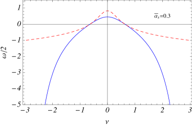
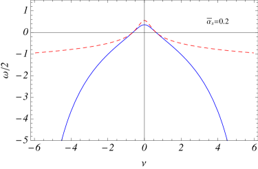
$(a)$	$(b)$

Figure 1: $\omega(\nu)$ for (a) $\bar{\alpha}_{s}=0.3$ and (b) $\bar{\alpha}_{s}=0.2$. LO and NLO are represented by dashed (red) and solid (blue) lines respectively. Notice the different $\nu$ ranges of the two plots.

with the explicit solution for $\omega$

$$\omega=\frac{2\bar{\alpha}_{s}\chi(\nu)}{1+2\bar{\alpha}_{s}\chi(\nu)}\,.$$ (61)

This solution is plotted in Fig. 1. $\omega$ diverges at $\nu=\nu^{*}$ satisfying $2\bar{\alpha}_{s}\chi(\nu^{*})=-1$. As $\bar{\alpha}_{s}\to 0$, $\omega$ approaches the LO expression while $\nu^{*}\to\pm\infty$. At $\gamma\to 0$, i.e. $i\nu\to 1/2$, $\chi\approx 1/(1-2i\nu)=1/2\gamma$ and (61) yields

$$\gamma(\omega)=\bar{\alpha}_{s}\left(\frac{1}{\omega}-1\right)\,.$$ (62)

This can be used as a model of anomalous dimension that takes into account the energy conservation as suggested in Ellis:1993rb ; AyalaFilho:1997du .

Integrating (59) over $\omega$ we obtain

$$N({\bm{r}},{\bm{b}},y)=\int_{-\infty}^{+\infty}d\nu\,C^{A}_{\nu}\,e^{\omega(\nu)y+\gamma\xi-\xi}\,,$$ (65)

with $\omega(\nu)$ given by (61). Remembering that in the dilute regime (and $N_{c}\gg 1$) $N_{G}=2N$, see (18), and using the same initial condition as in (23) we get

$$N_{G}({\bm{r}},{\bm{b}},y)=\int_{-\infty}^{\infty}d\nu\,\exp\left\{\frac{2\bar{\alpha}_{s}\chi(\nu)y}{1+2\bar{\alpha}_{s}\chi(\nu)}\right\}\,(rQ_{s0})^{1+2i\nu}\,\frac{1}{8\pi}\frac{1+(1-2i\nu)\ln\frac{Q_{s0}}{\Lambda}}{(1-2i\nu)^{2}}\,.$$ (66)

This integral can be taken in the double-logarithmic approximation (DLA), which corresponds to keeping only one of the poles of $\chi$, namely $\chi(\nu)=1/(1-2i\nu)$. Denote

$$\phi(\xi,y)=\frac{2\bar{\alpha}_{s}\chi(\nu)y}{1+2\bar{\alpha}_{s}\chi(\nu)}-(1/2+i\nu)\xi\,.$$ (67)

Then, in the DLA

$$\phi(\xi,y)\approx\frac{\bar{\alpha}_{s}}{\gamma+\bar{\alpha}_{s}}y+\gamma\xi-\xi=2\sqrt{\bar{\alpha}_{s}y\xi}-\xi(1+\bar{\alpha}_{s})+\frac{1}{2}\left(\gamma-\gamma_{0}\right)^{2}\frac{2\xi^{3/2}}{(\bar{\alpha}_{s}y)^{1/2}}\,,$$ (68)

where

$$\gamma_{0}=\sqrt{\frac{\bar{\alpha}_{s}y}{\xi}}-\bar{\alpha}_{s}$$ (69)

is the saddle point. Substituting (68) into (66) and integrating over the saddle point gives

$$N_{G}({\bm{r}},{\bm{b}},y)=\frac{1+2\gamma_{0}\ln\frac{Q_{s0}}{\Lambda}}{32\pi^{1/2}\gamma_{0}^{2}}\frac{(\bar{\alpha}_{s}y)^{1/4}}{\ln^{3/4}\frac{1}{r^{2}Q_{s}^{2}}}(r^{2}Q_{s}^{2})^{1+\bar{\alpha}_{s}}e^{2\sqrt{\bar{\alpha}_{s}y\ln\frac{1}{r^{2}Q_{s}^{2}}}}\,.$$ (70)

The most important correction due to energy conservation requirement is steeper dependence of the scattering amplitude on $r$.

VI.1.2 Saturation momentum

To determine the saturation momentum, we need to find a set of lines in the $y,\xi$ plane along which the amplitude is constant. In the DLA approximation this is equivalent to the requirement that the phase (68) be constant, i.e. $2\sqrt{\bar{\alpha}_{s}y\xi}-\xi(1+\bar{\alpha}_{s})=0$. Denoting solution to this equation as $\xi_{s}(y)$ we obtain

$$Q_{s}^{2}=Q_{s0}^{2}e^{\xi_{s}}=Q_{s0}^{2}\,e^{\frac{4\bar{\alpha}_{s}y}{(1+\bar{\alpha}_{s})^{2}}}\,.$$ (71)

Energy dependence of the saturation momentum becomes more gradual compared to the LO.

A more accurate evaluation of the saturation momentum requires solving the following two equations Mueller:2002zm :

$$\phi=\frac{2\bar{\alpha}_{s}\chi(\gamma)y}{1+2\bar{\alpha}_{s}\chi(\gamma)}+\gamma\xi-\xi\,=0$$ (72a)

$$\frac{\partial\phi}{\partial\gamma}=\frac{2\bar{\alpha}_{s}\chi^{\prime}(\gamma)y}{1+2\bar{\alpha}_{s}\chi(\gamma)}-\frac{(2\bar{\alpha}_{s})^{2}\chi(\gamma)\chi^{\prime}(\gamma)y}{(1+2\bar{\alpha}_{s}\chi(\gamma))^{2}}+\xi=0\,.$$ (72b)

The first one determines the line on $y,\xi$ plane where the amplitude is stationary, while the second one fixes the trajectory of the steepest descend Mueller:2002zm . Eliminating $y$ and $\xi$ from these equations we end up with an equation for the saddle-point $\gamma_{\text{sp}}$:

$$\chi^{\prime}(\gamma_{\text{sp}})+\frac{1}{1-\gamma_{\text{sp}}}\chi(\gamma_{\text{sp}})=\frac{2\bar{\alpha}_{s}\chi(\gamma_{\text{sp}})\chi^{\prime}(\gamma_{\text{sp}})}{1+2\bar{\alpha}_{s}\chi(\gamma_{\text{sp}})}\,.$$ (73)

Employing (6) we write

$$\chi(\gamma)=\psi(1)-\frac{1}{2}\psi(\gamma)-\frac{1}{2}\psi(1-\gamma)\,,$$ (74)

$$\chi^{\prime}(\gamma)=-\frac{1}{2}\psi^{\prime}(\gamma)+\frac{1}{2}\psi^{\prime}(1-\gamma)\,.$$ (75)

Saddle point in the LO is obtained as the solution to (73) in the $\bar{\alpha}_{s}\to 0$ limit. Hence, dropping the r.h.s. of (73) we obtain $\gamma_{\text{sp}}=0.37$. In the NLO approximation $\gamma_{\text{sp}}$ depends on $\bar{\alpha}_{s}$ as shown in Fig. 2(a). As $\bar{\alpha}_{s}$ increases $\gamma_{\text{sp}}$ decreases and becomes closer to the experimental data. For a given $\bar{\alpha}_{s}$ (72) implies that

$$Q_{s}^{2}=Q_{s0}^{2}\exp\left\{\frac{1}{1-\gamma_{\text{sp}}}\frac{2\bar{\alpha}_{s}\chi(\gamma_{\text{sp}})y}{1+2\bar{\alpha}_{s}\chi(\gamma_{\text{sp}})}\right\}\equiv Q_{s0}^{2}e^{2\bar{\alpha}_{s}y\,h(\bar{\alpha}_{s})}\,,$$ (76)

Particularly, at the LO $h(\bar{\alpha}_{s})=\frac{\chi(\gamma_{\text{sp}})}{1-\gamma_{\text{sp}}}=2.44$ independently of $\bar{\alpha}_{s}$. In Fig. 2(b) we show the NLO behavior of $h$ as given by (76) and its DLA given by (71). Again we observe that the NLO correction makes the energy dependence of the saturation scale more gradual. This is understandable because the energy conservation reduces the phase space available for gluon emission.

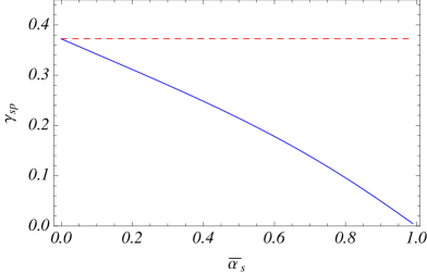
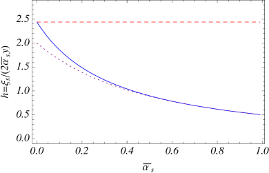
$(a)$	$(b)$

Figure 2: (a) Solution for the saddle point equation (73) $\gamma_{\text{sp}}(\bar{\alpha}_{s})$: solid blue line is NLO (energy conservation), dashed red line is LO. (b) Function $h(\bar{\alpha}_{s})$ defined in (76): solid blue line is NLO, dotted (purple) is its DLA (71) and dashed (red) is LO.

VI.1.3 Saturation regime

In the saturation region, (VI.1) reads

$$\frac{\partial N({\bm{r}},{\bm{b}},y)}{\partial y}=\bar{\alpha}_{s}\left(1-\frac{\partial}{\partial y}\right)\int_{2/Q_{s}^{2}}^{r^{2}}\frac{dr^{\prime 2}}{r^{\prime 2}}\left\{N({\bm{r}}^{\prime},{\bm{b}},y)-N({\bm{r}}^{\prime},{\bm{b}},y)N({\bm{r}},{\bm{b}},y)\right\}$$ (77)

We expect that the scattering amplitude will approach its unitarity limit as $y\to\infty$. Therefore, we are looking for a solution to (77) in the form

$$N=1-S$$ (78)

where $S\ll 1$ is an element of the scattering-matrix of dipole ${\bm{r}}$. Now

$$-\frac{\partial S(r,y)}{\partial y}=\bar{\alpha}_{s}\left(1-\frac{\partial}{\partial y}\right)\left\{\ln(r^{2}Q_{s}^{2})S(r,y)\right\}\,.$$ (79)

We are interested in the scaling solution viz. we are looking for a solution in the form $S(r,y)=S(\tau(r,y))$ where

$$\tau=\ln(r^{2}Q_{s}^{2})=\ln(r^{2}Q_{s0}^{2})+\frac{4\bar{\alpha}_{s}y}{(1+\bar{\alpha}_{s})^{2}}\,,$$ (80)

and we used (71). Introducing a new parameter that determines rapidity dependence of the saturation scale (in the DLA)

$$\lambda=\frac{4\bar{\alpha}_{s}}{(1+\bar{\alpha}_{s})^{2}}$$ (81)

we write (79) as

$$\frac{\partial S}{\partial\tau}(\bar{\alpha}_{s}\lambda\tau-\lambda)=\bar{\alpha}_{s}(\tau-\lambda)S\,.$$ (82)

It is easily integrated with the solution

$$S(\tau)=S_{0}e^{\frac{\tau}{\lambda}}(1-\bar{\alpha}_{s}\tau)^{\frac{1}{\bar{\alpha}_{s}\lambda}-1}\,,$$ (83)

where $S_{0}$ is an integration constant that is determined by matching with the solution in the dilute regime. This is similar to the solution derived in Kormilitzin:2010at . Note, that (83) is applicable only at $1<\tau\leq 1/\bar{\alpha}_{s}$. Solution (83) is exhibited in Fig. 3.

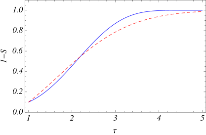
Figure 3: Solution to the LO (dashed red line) and the modified (solid blue) BK equations deeply in the saturation region $1<\tau<1/\bar{\alpha}_{s}$. The initial condition is $S=0.9$ at $\tau=1$.

VI.2 Dipole density

We proceed with the analysis of the NLO effects related to the energy conservation in the dipole density. Using the result of the Sec. VI.1 we obtain in place of (9):

$$\tilde{f}({\bm{r}},{\bm{q}},y)=\frac{r}{\pi q}\int_{-\nu^{*}}^{\nu^{*}}d\nu\,\exp\left\{\frac{2\bar{\alpha}_{s}\chi(\nu)y}{1+2\bar{\alpha}_{s}\chi(\nu)}\right\}\,\left(\frac{rq}{2}\right)^{2i\nu}\frac{\Gamma\left(\frac{1}{2}-i\nu\right)}{\Gamma\left(\frac{1}{2}+i\nu\right)(2i\nu+1)^{2}}\,,$$ (84)

where $\nu^{*}$ satisfy $1+2\bar{\alpha}_{s}\chi(\nu^{*})=0$. Similarly to our discussion in Sec. III.1, we would like to find asymptotic expressions for $\tilde{f}$ in various kinematic regions. Since the integrand in (84) is a steeply falling function of $\nu$ we can replace the limits of integration by $\nu^{*}=\pm\infty$.

1. $\alpha_{s}y\gg\ln^{2}\frac{rq}{2}$. Expression in the exponent of (84) can be approximated as

   $$\frac{2\bar{\alpha}_{s}\chi(\nu)y}{1+2\bar{\alpha}_{s}\chi(\nu)}\approx\frac{(\alpha_{P}^{(0)}-1)y}{\alpha_{P}^{(0)}}-\frac{14\zeta(3)\bar{\alpha}_{s}y}{[\alpha_{P}^{(0)}]^{2}}\nu^{2}\,.$$ (85)

   We see that the pomeron intercept became $\alpha_{P}^{(1)}=2-1/\alpha_{P}^{(0)}$, while the “diffusion constant” has increased by $1/[\alpha_{P}^{(0)}]^{2}$, i.e. growth of $\tilde{f}$ with rapidity has slowed down, while diffusion has speeded up. The later observation has profound implications on diffractive gluon production (see Li:2008bm ; Li:2008jz ; Li:2008se for in-depth discussion). For $\bar{\alpha}_{s}=0.4$ the intercept is $\alpha_{P}^{(1)}=1.5$ (compare with $\alpha_{P}^{(0)}=2.1$), which is in better agreement with the data. Eq. (13) is modified as follows

   $$\tilde{f}({\bm{r}},{\bm{q}},y)=\frac{r}{q}\frac{\alpha_{P}^{(0)}}{\sqrt{14\pi\zeta(3)\bar{\alpha}_{s}\,y}}\,e^{(\alpha_{P}^{(1)}-1)y}\,e^{-\frac{[\alpha_{P}^{(0)}]^{2}\ln^{2}\frac{rq}{2}}{14\zeta(3)\bar{\alpha}_{s}\,(Y-y)}}\,.$$ (86)

2. $rq<2$ and $\ln\frac{2}{rq}\gg\alpha_{s}y$. Expanding $\chi\approx 1/(1-2i\nu)$ we find the saddle point at

   $$2i\nu_{1}=1+2\bar{\alpha}_{s}-\sqrt{\frac{2\bar{\alpha}_{s}y}{\ln\frac{2}{rq}}}\,.$$ (87)

   Integration over the saddle-point and assuming $\ln\frac{2}{rq}\ll y/\alpha_{s}$ yields

   $$\tilde{f}({\bm{r}},{\bm{q}},y)=\frac{r^{2}}{8\sqrt{\pi}}\frac{(rq/2)^{2\bar{\alpha}_{s}}}{\left(2\bar{\alpha}_{s}y\ln\frac{2}{rq}\right)^{1/4}\left[1-\sqrt{2\bar{\alpha}_{s}\frac{1}{y}\ln\frac{2}{rq}}\right]}e^{2\sqrt{2\bar{\alpha}_{s}y\ln\frac{2}{rq}}}\,.$$ (88)

3. $rq>2$ and $\alpha_{s}y\ll\ln\frac{rq}{2}\ll y/\alpha_{s}$. Now, another pole in $\chi$ dominates $\chi\approx 1/(1+2i\nu)$ with the result

   $$\tilde{f}({\bm{r}},{\bm{q}},y)=\frac{1}{2q^{2}\sqrt{\pi}}\frac{(2/rq)^{2\bar{\alpha}_{s}}}{\left(2\bar{\alpha}_{s}y\ln\frac{rq}{2}\right)^{1/4}\left[1-\sqrt{2\bar{\alpha}_{s}\frac{1}{y}\ln\frac{rq}{2}}\right]}e^{2\sqrt{2\bar{\alpha}_{s}y\ln\frac{rq}{2}}}\,.$$ (89)

Note, that in both cases (88) and (89) the momentum dependence of the leading twist is modified by an additional power $2\bar{\alpha}_{s}$. This can have important consequences at high $Q^{2}$ and/or $k_{T}$. We are discussing this in more detail in Sec. VIII.

VII Nuclear modification factor

The nuclear modification factor is defined as

$$R_{\gamma^{*}A}=\frac{\int d^{2}b\,\frac{d\sigma_{\gamma^{*}A}}{d^{2}k\,dy\,d^{2}b}}{A\,\int d^{2}b\,\frac{d\sigma_{\gamma^{*}p}}{d^{2}k\,dy\,d^{2}b}}\,.$$ (90)

In the logarithmic approximation (56) implies that the cross section for inclusive gluon production in DIS on a heavy nucleus is simply proportional to the cross section for inclusive gluon production by dipole of size $r=2/Q$. Consequently, the nuclear modification factor (90) can be approximated by

$$R_{\gamma^{*}A}\approx R_{q\bar{q}+A}\big{|}_{r=2/Q}\,.$$ (91)

In the same approximation, $pA$ scattering can also be approximated as the $q\bar{q}+A$ one provided that we are interested in inclusive processes not too close in rapidity to the proton or nucleus fragmentation region Li:2008se . Atomic weight $A$ and rapidity $y$ dependence of incluisve cross section in $pA$ collisions at the leading logarithmic order was discussed in great detail in Kharzeev:2003wz and we refer the interested reader to that paper. Here we will focus on the logarithmic derivative of the nuclear modification factor defined as

$$J=\frac{1}{R_{\gamma^{*}A}}\frac{\partial R_{\gamma^{*}A}}{\partial y}\,.$$ (92)

Outside the saturation region this observable is proportional to the difference between the anomalous dimension of the gluon distribution in the nucleus $\gamma^{A}$ and the one in the proton $\gamma^{p}$. If the coherence effects were negligible, the two anomalous dimensions would have been identical. This is not the case according to the theory of gluon saturation. As the result, the NMF is suppressed even at $k_{T}>Q_{s}$. Thus $J$ is especially sensitive probe of the mechanism that leads to the suppression of the NMF for hadron production at small $x$.

Let us relate $J$ to the difference of anomalous dimensions $\gamma^{A}-\gamma^{p}$. It follows from (90) that

$$J=\frac{\partial}{\partial y}\ln R_{\gamma^{*}A}=\frac{\partial}{\partial y}\ln\frac{d\sigma^{\gamma^{*}A}}{d^{2}k\,dy}-\frac{\partial}{\partial y}\ln\frac{d\sigma^{\gamma^{*}p}}{d^{2}k\,dy}\,.$$ (93)

Using (91) and (30),(31) and assuming that the $b$-dependence factors out we derive

$$\frac{\partial}{\partial y}\ln R_{\gamma^{*}A}\approx\frac{\partial}{\partial y}\ln g^{A}\big{|}_{{\bm{b}}=0}-\frac{\partial}{\partial y}\ln g^{p}\big{|}_{{\bm{b}}=0}\,,$$ (94)

where $g$ is the inclusive $q\bar{q}+A$ cross section modulo a constant factor, see Sec. IV. We assigned superscripts $A$ and $p$ to $g$ to indicate the two cases: $A>1$ and $A=1$ respectively. In the following we will omit the specification that $g$ is taken at zero impact parameter. Outside the saturation region we can employ the Mellin representation for $N_{G}$ (23) and $\tilde{f}$ (9), substitute them into (31), take the LLA limit and obtain up to a pre-exponential factor

$$g^{A}\propto Q_{0}r\,\exp\left[2\bar{\alpha}_{s}\chi(\nu_{0})(Y-y)+2i\nu_{0}\ln\frac{rp}{2}+2\bar{\alpha}_{s}\chi(\mu_{0}^{A})y+2i\mu_{0}^{A}\ln\frac{Q_{s0}}{p}\right]$$ (95)

and analogously for $g^{p}$. Here $\nu_{0}$, $\mu_{0}^{A}$ are the saddle points in the Mellin transform of $\tilde{f}$ and $\tilde{N}_{G}$ respectively. The omitted pre-factor in (95) depends on momenta only logarithmically. Momentum $p$ stands for either $Q$ or $k$ depending on the kinematic region of interest. It is straightforward to verify that $g^{A}$ and $g^{p}$ obey the equations

$$\frac{\partial g^{A}}{\partial y}=2\bar{\alpha}_{s}[\chi(\mu_{0}^{A})-\chi(\nu_{0})]g^{A}\,,\qquad\frac{\partial g^{p}}{\partial y}=2\bar{\alpha}_{s}[\chi(\mu_{0}^{p})-\chi(\nu_{0})]g^{p}\,.$$ (96)

This is just the Mellin transform of the BFKL equation. Plugging (96) into (94) we derive

$$J=2\bar{\alpha}_{s}\left[\chi(\mu_{0}^{A})-\chi(\mu_{0}^{p})\right]\approx 2\bar{\alpha}_{s}\chi^{\prime}(\gamma_{0}^{p})\,\left(\gamma_{0}^{A}-\gamma_{0}^{p}\right)\,.$$ (97)

$\chi^{\prime}(\gamma)$ is given by (75) and the saddle point $\gamma_{0}^{p}$ satisfies (73).

Consider a few examples. Denote $p=\max\{k_{T},Q\}$. In the region $\ln\frac{p}{Q_{s0}}\gg\bar{\alpha}_{s}y$ we have (see e.g. (15) and (24))

$$\chi\approx\frac{1}{1-2i\mu}=\frac{1}{2\gamma}$$ (98)

with the saddle point

$$\gamma^{A}=\frac{1}{2}(1-2i\mu_{0}^{A})=\frac{1}{2}\sqrt{\frac{2\bar{\alpha}_{s}y}{\ln\frac{p}{\Lambda}+\ln\frac{\Lambda}{Q_{s0}}}}\approx\frac{1}{2}\sqrt{\frac{2\bar{\alpha}_{s}y}{\ln\frac{p}{\Lambda}}}\left(1+\frac{\ln\frac{Q_{s0}}{\Lambda}}{2\ln\frac{p}{\Lambda}}\right)$$ (99)

$\gamma^{p}$ is obtained by setting $Q_{s0}=\Lambda$. We see that in this kinematic region $\gamma^{p}<\gamma^{A}$. By dint of (98) $\chi^{\prime}(\gamma)<0$ implying that $J<0$. More precisely,

$$J=-\bar{\alpha}_{s}\frac{\ln\frac{Q_{s0}}{\Lambda}}{\sqrt{2\bar{\alpha}_{s}y\ln\frac{p}{\Lambda}}}\,.$$ (100)

In the saturation region $\ln\frac{p}{Q_{s0}}\ll\bar{\alpha}_{s}y$, $\gamma^{A}$ effectively tends to zero as the dipole scattering amplitude saturates at unity. Therefore, in that region $\gamma^{A}<\gamma^{p}$, while $\chi\approx\frac{1}{2(1-\gamma)}$. Hence $\chi^{\prime}(\gamma)>0$ implying that again $J<0$. Finally, in the diffusion region $\chi\approx 2\ln 2-7\zeta(3)\nu^{2}$ and we similarly obtain

$$J=-\frac{\ln\frac{p}{\Lambda}\ln\frac{Q_{s0}}{\Lambda}}{7\zeta(3)\bar{\alpha}_{s}y^{2}}\,.$$ (101)

Negativity of $J$ in all kinematic regions signifies the decrease of the inclusive cross section as a function of rapidity. The rate of the decrease depends on the absolute value of $J$.

VIII Numerical analysis

The numerical calculation of the inclusive hadron production is performed using Eqs. (1),(2),(11),(10). We employed the bGCG model Kowalski:2006hc for the forward dipole–nucleus scattering amplitude. The bCGC model is reviewed in Appendix. Function $\tilde{f}$ is calculated using formula (84). The gluon spectrum is then convoluted with the LO pion fragmentation function $\mathcal{F}_{G}$ as follows

$$\frac{d\sigma_{\pi}}{d^{2}k\,dy}=\int_{z_{\text{min}}}^{1}\frac{dz}{z^{2}}\,\frac{d\sigma_{G}}{d^{2}k\,dy}(k/z)\,\mathcal{F}_{G}(z,k)\,.$$ (102)

The fragmentation function is given in Kniehl:2000hk . The total rapidity interval is taken to be $Y=10$, which is equivalent to $x=e^{-Y}=4.5\cdot 10^{-5}$. The range of photon virtualities that we consider is $Q^{2}=2-37$ GeV². This kinematic region can be probed at the proposed Large Hadron electron Collider and its low $Q^{2}$ part at the Electron Ion Collider Boer:2011fh . The rapidity interval $y$ from the nucleus to the produced gluon is related to $x_{\text{I\!P}}$, a variable used in differctive DIS, as $x_{\text{I\!P}}=e^{-y}$. We consider $y$ in a narrow interval $5\leq y\leq 7$ allowed by our formalism. At larger $x$ and/or $x_{\text{I\!P}}$ the validity of the leading logarithmic approximation that we employ becomes uncertain.

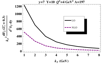
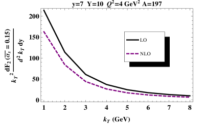
$(a)$	$(b)$

Figure 4: Comparison between the LO and NLO calculations of $k^{2}\frac{dF_{2}(x,Q^{2};y)}{d^{2}kdy}$ as a function of $k_{T}$ at two values of coupling (a) $\bar{\alpha}_{s}=0.3$ and (b) $\bar{\alpha}_{s}=0.15$.

The results of our calculations are shown in Figs.(4)–(8). The NLO calculation shown in the figures refers to the part of the NLO terms that are responsible for energy conservation. In Fig. 4,5 we plot the inclusive cross section normalized in the same way as the structure function

$$\frac{dF_{2}(x,Q^{2};y)}{d^{2}kdy}=\frac{1}{\alpha_{em}}\frac{Q^{2}}{4\pi^{2}}\frac{d\sigma^{\gamma*A}(x,Q^{2};y)}{d^{2}kdy}\,.$$ (103)

We observe that inclusive gluon production at NLO is suppressed compared with the LO case. This is because the anomalous dimension of dipole density at NLO is smaller compared with that of LO, as can be seen in Fig. 2. This is expected since energy conservation constrains the phase space available for hadron production. In Fig. 4 we demonstrate that the difference between the LO and NLO calculation is smaller at smaller values of coupling.

We see in Fig. 5(b) that at small $k_{T}$, the gluon production cross section follows $1/k_{T}^{2}$ behavior. Indeed, $1/k_{T}^{2}$ comes from the Lipatov vertex, whereas the gluon distribution in the nucleus is saturated and hence depends on momentum $k_{T}$ only logarithmically. This is seen in (11) where at small $k_{T}$ the integral tends to a constant leaving the $1/k_{T}^{2}$ pre-factor in front. Modification of the gluon spectrum due to fragmentation can be inferred by comparing Fig. 5(a) and (b).

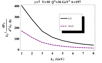
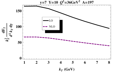
$(a)$	$(b)$

Figure 5: Inclusive spectrum $k^{2}\frac{dF_{2}(x,Q^{2};y)}{d^{2}kdy}$ of (a) pions, (b) gluons as a function of $k_{T}$.

The cross section grows with $Q^{2}$ and $x_{\text{I\!P}}$ logarithmically; both dependences are much steeper at the LO than in the NLO. We also note that energy conservation correction substantially reduces the cross section. However, the functional form of the $k_{T}$-spectrum does not change in the kinematic region that we studied, as we checked explicitly. We attribute this to that fact that the dominant contribution to the Mellin transform stems from anomalous dimension $\gamma\approx 1/2$ in both cases. We expect that at much larger $Q$ and $k_{T}$ the NLO $k_{T}$-spectrum becomes steeper than those in LO due to additional factors $1/Q^{2\bar{\alpha}_{s}}$ or $1/k_{T}^{2\bar{\alpha}_{s}}$. However, assumptions of our model restrict our calculation only to the semi-hard values of transverse momenta.

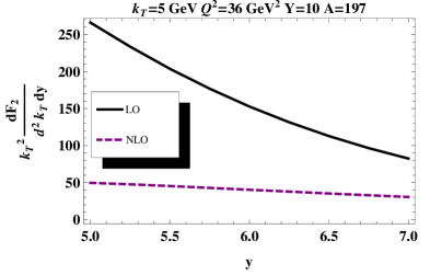
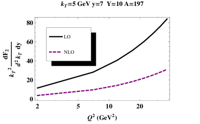
$(a)$	$(b)$

Figure 6: Inclusive hadron spectrum $k^{2}\frac{dF_{2}(x,Q^{2};y)}{d^{2}kdy}$ as a function of (a) $y$, (b) $Q^{2}$.

The largest uncertainty in our numerical calculation of hadron spectrum comes from the oversimplified treatment of nuclei geometry. Instead of integrating with a realistic nuclear thickness $T(b)$ we approximated the nuclear density by the step-function. Based on our previous experience with this type of numerical calculations we expect that a more accurate treatment of the nuclear density will only affect the overall normalization of the cross section. From this perspective the ratios of the inclusive spectra should not be much affected by this uncertainty.

Our calculation of the Nuclear Modification Factor (NMF) as a function of $k_{T}$ for Au ($A=197$) and Ca ($A=40$) is displayed in Fig. 7. The general feature of NMF is suppression at low $k_{T}$ and enhancement at larger $k_{T}$ (the later is often referred to as the Cronin effect). This is in contrast with the hadron production in $pA$ scattering where the Cronin effect gives way to the suppression at all $k_{T}$’s provided that the hadron rapidity $y$ is large enough. The reason for this difference is that whereas $pA$ scattering can be approximated by dipole-nucleus scattering Li:2008se , $\gamma^{*}A$ interaction is a superposition of many dipole-nucleus scatterings with different dipole sizes $r$, see (3). At small $k_{T}$ NMF for dipoles of all sizes is suppressed Kharzeev:2003wz and therefore we observe suppression of the resulting $R$ for DIS. On the other hand, the fact that $R>1$ at large $k_{T}$ implies that the inclusive cross section in that region is dominated by dipoles whose individual scattering on the nucleus exhibits Cronin enhancement, i.e. they are not much effected by the low-$x$ evolution. Presence of such dipoles is ensured by evolution of the dipole density $n$, which happens if $Y-y\gg 1$. Comparing Figs.7 (a)-(c) with (d) we note that due to fragmentation, NMF of hadrons is much slower function of $Q^{2}$, $y$ and $k_{T}$ than NMF of gluons. Additonally, fragmentation shifts the value of the transverse momentum at which NMF crosses unity towards lower $k_{T}$.

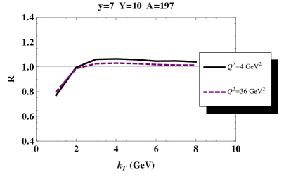
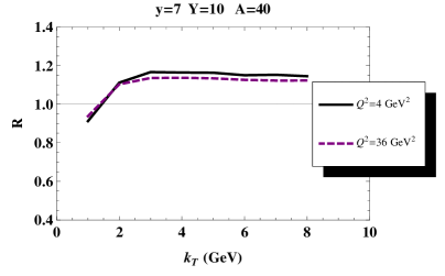
$(a)$	$(b)$
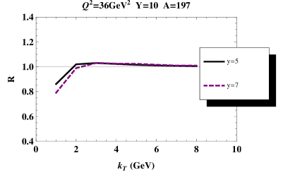
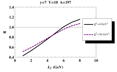
$(c)$	$(d)$

Figure 7: Nuclear Modification Factor as a function of $k_{T}$ for (a)-(c) hadrons at various $A$, $y$ and $Q^{2}$; (d) gluons. All calculations include the NLO effects.

Another feature seen in Fig. 7 (especially (d)) is that suppression of NMF at low $k_{T}$ and its enhancement at high $k_{T}$ increases with the photon virtuality $Q^{2}$. To understand the $Q^{2}$ dependence of the NMF we note that a typical term in its twist expansion looks like

$$R\sim\left(\frac{1}{Q^{2}}\right)^{n(\gamma_{A}-\gamma_{p})}\,,$$ (104)

where $n\geq 1$ is an integer number. It implies that

$$\frac{\partial R}{\partial\ln Q^{2}}\approx-n(\gamma_{A}-\gamma_{p})R.$$ (105)

At large $k_{T}$ $\gamma^{A}>\gamma^{p}$ thus $\frac{\partial R}{\partial\ln Q^{2}}<0$, whereas at small $k_{T}$ $\gamma^{A}<\gamma^{p}$ thus $\frac{\partial R}{\partial\ln Q^{2}}>0$. This is indeed what we observe in Fig. 7. Dependence of NMF on $y$ can be explained similarly.

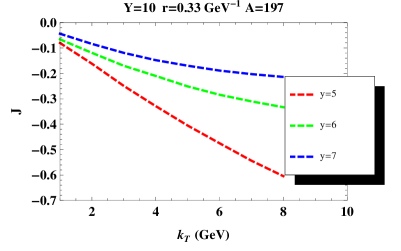
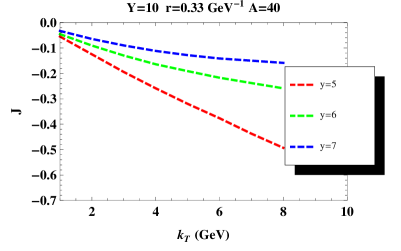
$(a)$	$(b)$
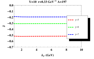
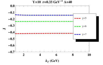
$(c)$	$(d)$

Figure 8: Logarithmic derivative of NMF for dipole-nuleus scattering as a function for $k_{T}$ for (a),(b) gluons, (c),(d) hadrons. dipole size $r$, total rapidity $Y$ and nuclear wight $A$ are indicated on each plot. All calculations include the NLO effects.

Fig. 8 displays the logarithmic derivative of the NMF $J$ defined in (92). As we argued in Sec. VII this quantity is proportional to the difference between the anomalous dimensions of the gluon distribution function in nucleus and proton, see(97). Our analysis in (100),(101) indicates that $J$ is negative and decreases as the hadron rapidity $y$ increases, which is indeed seen in Fig. 8. Similar trend has been noticed in $pA$ collisions in Tuchin:2007pf . We can also see the effect of fragmentation on $J$ by comparing Fig. 8(a),(b) with (c),(d). It is interesting that fragmentation completely erases the $k_{T}$ dependence, while leaving the $y$ dependence qualitatively similar. We think that experimental investigation of $J$ is of great interest as it emphasizes the difference between the (linear) gluon evolution in a heavy nucleus and in proton.

IX Summary

In this paper we studied the inclusive hadron production in DIS scattering at small $x$ using the dipole model Mueller:1989st . We presented the analytical formulas for the cross section in various kinematic regions and discussed the role of the energy conservation, which is perhaps the most important NLO correction. Employing the modified BK equation suggested in Kormilitzin:2010at ; Gotsman:2004xb , we derived the corresponding correction to the pomeron intercept and found that it is numerically closer to the phenomenological value than the LO result. We also computed the high energy asymptotic of the forward dipole-nucleus scattering amplitude.

Motivated by possible low $x$ DIS experiments with heavy nuclei Boer:2011fh we performed numerical calculations of the DIS inclusive cross section using the bCGC model Kowalski:2006hc . The results are shown in Figs. 4–8. We noticed that the NLO effects generally tend to reduce the cross section and make it weaker function of its arguments as compared to the LO result. The nuclear modification factor exhibits suppression at low $k_{T}$ and enhancement at higher $k_{T}$ even at the largest hadron rapidities that we can address in our approach. To understand dependence of the NMF on rapidity better we introduced the logarithmic derivative of NMF $J$ and showed that it is proportional to the difference between the anomalous dimension of the gluon distribution function in nucleus and proton. Since this difference is non-vanishing only due to coherence effects, $J$ provides a direct measure of the effect of coherence on inclusive cross section. Figs. 7,8 show dependence of NMF and $J$ on the photon virtuality $Q^{2}$, $x$ and hadron rapidity $y$. We believe that our results may be helpful for experimental investigation of the low-$x$ regime of QCD in DIS.

Appendix A bCGC model

We performed the numerical calculations using the bCGC model of the forward dipole scattering amplitude Kowalski:2006hc . We treat the nuclei and proton profiles as step-functions; the saturation scales are assumed to scale with $A$ as $Q_{s}^{2}\propto A^{1/3}$. The advantage of this model – besides its compliance with the known analytical approximations to the BK equation Iancu:2002tr – is that its parameters are fitted to the low $x$ DIS data. The explicit form of the scattering amplitude $N$ is given by

$$N({\bm{r}},0,y)=\,\left\{\begin{array}[]{cc}\mathcal{N}_{0}\left(\frac{r^{2}\mathcal{Q}_{s}^{2}}{4}\right)^{\gamma}\,,&\quad r\mathcal{Q}_{s}\leq 2;\\ 1-\exp[-a\ln^{2}(br\mathcal{Q}_{s})]\,,&\quad r\mathcal{Q}_{s}\geq 2\,,\end{array}\right.$$ (106)

where $\mathcal{Q}_{s}^{2}$ is the the quark saturation scale related to the gluon saturation scale $Q_{s}^{2}$ – which we have called simply the ‘saturation scale’ throughout the paper – by $\mathcal{Q}_{s}^{2}=(4/9)Q_{s}^{2}$. Its functional form is

$$\mathcal{Q}_{s}^{2}=A^{1/3}x_{0}^{\lambda}\,e^{\lambda y}\,s^{\lambda/2}\,\mathrm{GeV}^{2}\,,$$ (107)

where $s$ is the square of the center-of-mass energy and $y$ is rapidity with respect to the central rapidity. The anomalous dimension is

$$\gamma=\gamma_{s}+\frac{1}{c\,\lambda\,(\ln\surd s+y)}\ln\left(\frac{2}{r\mathcal{Q}_{s}}\right)\,.$$ (108)

The gluon dipole scattering amplitude can be calculated using (18). Parameters $\gamma_{s}=0.628$ and $c=9.9$ follow from the BFKL dynamics Iancu:2002tr , while $\mathcal{N}_{0}=0.7$ and $\lambda=0.28$ are fitted to the DIS data. Constants $a$ and $b$ are uniquely fixed from by the requirement of continuity of the amplitude and its first derivative.

References

- (1) L. V. Gribov, E. M. Levin and M. G. Ryskin, Phys. Rept. 100, 1 (1983).
- (2) E.M. Levin and M.G Ryskin, Nucl. Phys. B304, 805 (1988); Sov. J. Nucl. Phys. 45, 150 (1987); 41, 300 (1985).
- (3) A. H. Mueller and J. -w. Qiu, Nucl. Phys. B 268, 427 (1986).
- (4) A. H. Mueller, Nucl. Phys. B 415, 373 (1994).
- (5) A. H. Mueller and B. Patel, Nucl. Phys. B 425, 471 (1994) [hep-ph/9403256].
- (6) A. H. Mueller, Nucl. Phys. B 437, 107 (1995) [hep-ph/9408245].
- (7) L. D. McLerran and R. Venugopalan, Phys. Rev. D 49, 3352 (1994) [arXiv:hep-ph/9311205].
- (8) L. D. McLerran and R. Venugopalan, Phys. Rev. D 49, 2233 (1994) [arXiv:hep-ph/9309289].
- (9) L. D. McLerran and R. Venugopalan, Phys. Rev. D 50 (1994) 2225 [arXiv:hep-ph/9402335].
- (10) Y. V. Kovchegov, Phys. Rev. D 54, 5463 (1996) [arXiv:hep-ph/9605446].
- (11) Y. V. Kovchegov, Phys. Rev. D 55, 5445 (1997) [arXiv:hep-ph/9701229].
- (12) J. Jalilian-Marian, A. Kovner, L. D. McLerran and H. Weigert, Phys. Rev. D 55, 5414 (1997) [arXiv:hep-ph/9606337].
- (13) J. Jalilian-Marian, A. Kovner, A. Leonidov and H. Weigert, Nucl. Phys. B 504 (1997) 415 [arXiv:hep-ph/9701284].
- (14) J. Jalilian-Marian, A. Kovner, A. Leonidov and H. Weigert, Phys. Rev. D 59, 014014 (1999) [arXiv:hep-ph/9706377].
- (15) J. Jalilian-Marian, A. Kovner and H. Weigert, Phys. Rev. D 59, 014015 (1999) [arXiv:hep-ph/9709432].
- (16) J. Jalilian-Marian, A. Kovner, A. Leonidov and H. Weigert, Phys. Rev. D 59, 034007 (1999) [Erratum-ibid. D 59, 099903 (1999)] [arXiv:hep-ph/9807462].
- (17) A. Kovner, J. G. Milhano and H. Weigert, Phys. Rev. D 62, 114005 (2000) [arXiv:hep-ph/0004014].
- (18) H. Weigert, Nucl. Phys. A 703, 823 (2002) [arXiv:hep-ph/0004044].
- (19) E. Iancu, A. Leonidov and L. D. McLerran, Nucl. Phys. A 692, 583 (2001) [arXiv:hep-ph/0011241].
- (20) E. Ferreiro, E. Iancu, A. Leonidov and L. McLerran, Nucl. Phys. A 703, 489 (2002) [arXiv:hep-ph/0109115].
- (21) Y. V. Kovchegov, Phys. Rev. D 60, 034008 (1999) [arXiv:hep-ph/9901281].
- (22) Y. V. Kovchegov, Phys. Rev. D 61, 074018 (2000) [arXiv:hep-ph/9905214].
- (23) I. Balitsky, Nucl. Phys. B 463, 99 (1996) [arXiv:hep-ph/9509348].
- (24) I. Balitsky, arXiv:hep-ph/9706411.
- (25) I. Balitsky, Phys. Rev. D 60, 014020 (1999) [arXiv:hep-ph/9812311].
- (26) E. Iancu and R. Venugopalan, arXiv:hep-ph/0303204.
- (27) J. Jalilian-Marian and Y. V. Kovchegov, Prog. Part. Nucl. Phys. 56, 104 (2006) [arXiv:hep-ph/0505052].
- (28) Y. V. Kovchegov and A. H. Mueller, Nucl. Phys. B 529, 451 (1998).
- (29) Y. V. Kovchegov and K. Tuchin, Phys. Rev. D 65, 074026 (2002).
- (30) M. A. Braun, Phys. Lett. B 483, 105 (2000) [arXiv:hep-ph/0003003].
- (31) A. Dumitru and L. D. McLerran, Nucl. Phys. A 700, 492 (2002) [arXiv:hep-ph/0105268].
- (32) J. P. Blaizot, F. Gelis, and R. Venugopalan, Nucl. Phys. A 743, 13 (2004) [arXiv:hep-ph/0402256].
- (33) D. Kharzeev, E. Levin, and L. McLerran, Phys. Lett. B 561, 93 (2003) [arXiv:hep-ph/0210332].
- (34) D. Kharzeev, Y. V. Kovchegov, and K. Tuchin, Phys. Rev. D 68, 094013 (2003) [arXiv:hep-ph/0307037].
- (35) D. Kharzeev, Y. V. Kovchegov, and K. Tuchin, Phys. Lett. B 599, 23 (2004) [arXiv:hep-ph/0405045].
- (36) R. Baier, A. Kovner, and U. A. Wiedemann, Phys. Rev. D 68, 054009 (2003) [arXiv:hep-ph/0305265].
- (37) E. Iancu, K. Itakura, and D. N. Triantafyllopoulos, Nucl. Phys. A 742, 182 (2004) [arXiv:hep-ph/0403103].
- (38) A. H. Mueller, Nucl. Phys. B 335, 115 (1990).
- (39) E. A. Kuraev, L. N. Lipatov, and V. S. Fadin, Sov. Phys. JETP 45, 199 (1977) [Zh. Eksp. Teor. Fiz. 72, 377 (1977)].
- (40) I. I. Balitsky and L. N. Lipatov, Sov. J. Nucl. Phys. 28 (1978) 822 [Yad. Fiz. 28 (1978) 1597].
- (41) V. S. Fadin and L. N. Lipatov, Phys. Lett. B 429, 127 (1998) [hep-ph/9802290].
- (42) M. Ciafaloni and G. Camici, Phys. Lett. B 430, 349 (1998) [hep-ph/9803389].
- (43) M. Ciafaloni, D. Colferai, G. P. Salam and A. M. Stasto, Phys. Rev. D 68, 114003 (2003) [hep-ph/0307188].
- (44) M. Ciafaloni, D. Colferai, G. P. Salam and A. M. Stasto, Phys. Rev. D 66, 054014 (2002) [hep-ph/0204282].
- (45) M. Ciafaloni, D. Colferai, G. P. Salam and A. M. Stasto, Phys. Lett. B 541, 314 (2002) [hep-ph/0204287].
- (46) J. R. Forshaw, D. A. Ross and A. Sabio Vera, Phys. Lett. B 498, 149 (2001) [hep-ph/0011047].
- (47) M. Ciafaloni, M. Taiuti and A. H. Mueller, Nucl. Phys. B 616, 349 (2001) [hep-ph/0107009].
- (48) S. J. Brodsky, V. S. Fadin, V. T. Kim, L. N. Lipatov and G. B. Pivovarov, JETP Lett. 70, 155 (1999) [hep-ph/9901229].
- (49) D. A. Ross, Phys. Lett. B 431, 161 (1998) [hep-ph/9804332].
- (50) E. Levin, hep-ph/9806228.
- (51) N. Armesto, J. Bartels and M. A. Braun, Phys. Lett. B 442, 459 (1998) [hep-ph/9808340].
- (52) Y. V. Kovchegov and A. H. Mueller, Phys. Lett. B 439, 428 (1998) [hep-ph/9805208].
- (53) E. Levin, Nucl. Phys. B 453, 303 (1995) [hep-ph/9412345].
- (54) M. A. Braun, Phys. Lett. B 348, 190 (1995) [hep-ph/9408261].
- (55) Y. V. Kovchegov and H. Weigert, Nucl. Phys. A 784, 188 (2007) [hep-ph/0609090].
- (56) Y. V. Kovchegov and H. Weigert, Nucl. Phys. A 789, 260 (2007) [hep-ph/0612071].
- (57) Y. V. Kovchegov and H. Weigert, Nucl. Phys. A 807, 158 (2008) [arXiv:0712.3732 [hep-ph]].
- (58) I. Balitsky, Phys. Rev. D 75, 014001 (2007) [hep-ph/0609105].
- (59) A. H. Mueller, D. N. Triantafyllopoulos, Nucl. Phys. B640, 331-350 (2002). [hep-ph/0205167].
- (60) D. N. Triantafyllopoulos, Nucl. Phys. B 648, 293 (2003) [hep-ph/0209121].
- (61) J. Kuokkanen, K. Rummukainen, H. Weigert, arXiv:1108.1867 [hep-ph].
- (62) H. Weigert, Nucl. Phys. A 783, 165 (2007).
- (63) G. Chachamis, M. Lublinsky and A. Sabio Vera, Nucl. Phys. A 748, 649 (2005) [hep-ph/0408333].
- (64) A. Kormilitzin and E. Levin, arXiv:1009.1468 [hep-ph].
- (65) E. Gotsman, E. Levin, U. Maor and E. Naftali, Nucl. Phys. A 750, 391 (2005) [arXiv:hep-ph/0411242].
- (66) E. Gotsman, E. Levin, M. Lublinsky and U. Maor, Eur. Phys. J. C 27, 411 (2003) [hep-ph/0209074].
- (67) H. Kowalski, L. Motyka and G. Watt, Phys. Rev. D 74, 074016 (2006) [arXiv:hep-ph/0606272].
- (68) N. N. Nikolaev and B. G. Zakharov, Z. Phys. C 49, 607 (1991).
- (69) Y. Li and K. Tuchin, Phys. Rev. D 77, 114012 (2008) [arXiv:0802.2954 [hep-ph]].
- (70) Y. Li and K. Tuchin, arXiv:0803.1608 [hep-ph].
- (71) Y. Li and K. Tuchin, Phys. Rev. C 78, 024905 (2008) [arXiv:0806.2087 [hep-ph]].
- (72) E. Levin and K. Tuchin, Nucl. Phys. B 573, 833 (2000) [hep-ph/9908317].
- (73) E. Levin and K. Tuchin, Nucl. Phys. A 691, 779 (2001) [arXiv:hep-ph/0012167].
- (74) E. Levin and K. Tuchin, Nucl. Phys. A 693, 787 (2001) [hep-ph/0101275].
- (75) R. K. Ellis, Z. Kunszt and E. M. Levin, Nucl. Phys. B 420, 517 (1994) [Erratum-ibid. B 433, 498 (1995)].
- (76) A. L. Ayala Filho, M. B. Gay Ducati and E. M. Levin, Nucl. Phys. B 511, 355 (1998) [arXiv:hep-ph/9706347].
- (77) C. Marquet and C. Royon, Phys. Rev. D 79, 034028 (2009) [arXiv:0704.3409 [hep-ph]].
- (78) K. Tuchin, Nucl. Phys. A 798, 61 (2008) [arXiv:0705.2193 [hep-ph]].
- (79) E. Iancu, K. Itakura and L. McLerran, Nucl. Phys. A 708, 327 (2002) [arXiv:hep-ph/0203137].
- (80) B. A. Kniehl, G. Kramer and B. Potter, Nucl. Phys. B 597, 337 (2001) [hep-ph/0011155].
- (81) D. Boer, M. Diehl, R. Milner, R. Venugopalan, W. Vogelsang, D. Kaplan, H. Montgomery and S. Vigdor et al., arXiv:1108.1713 [nucl-th].