Quantum walk on distinguishable non-interacting many-particles and indistinguishable two-particle

Abstract

We present an investigation of many-particle quantum walks in systems of non-interacting distinguishable particles. Along with a redistribution of the many-particle density profile we show that the collective evolution of the many-particle system resembles the single-particle quantum walk evolution when the number of steps is greater than the number of particles in the system. For non-uniform initial states we show that the quantum walks can be effectively used to separate the basis states of the particle in position space and grouping like state together. We also discuss a two-particle quantum walk on a two-dimensional lattice and demonstrate an evolution leading to the localization of both particles at the center of the lattice. Finally we discuss the outcome of a quantum walk of two indistinguishable particles interacting at some point during the evolution.

I Introduction

The idea of a quantum walk, the quantum analog of the classical random walk, dates back to 1958 Ria58 and 1965 FH65 but the concept was formally developed only in 1990’s ADZ93 ; DM96 ; FG98 . In a one-dimensional situation a quantum walk evolving in position space spreads quadratically faster than its classical counterpart, due to the interference of amplitudes of the multiple paths ABN01 ; NV01 . This was found to have interesting applications in quantum information theory, allowing for efficient quantum algorithms Amb03 ; CCD03 ; SKB03 ; AKR05 . However, quantum walks have also been shown the be useful for coherent quantum control over atoms and quantum phase transitions CL08 , to explain breakdown phenomena in electric-field driven systems OKA05 , to give direct experimental evidence for wavelike energy transfer within photosynthetic systems ECR07 ; MRL08 , to generate entanglement between two spatially separated system CGB10 and to generate topological phases KRB10 . Experimental implementation of quantum walks have been reported using nuclear magnetic resonance (NMR) DLX03 ; RLB05 , continuous tunneling of light fields through waveguide lattices PLP08 , the phase space of trapped ions SMS09 ; ZKG10 , single optically trapped neutral atoms KFC09 and single SCP10 ; BFL10 and two-photon systems PLM10 ; OBB11 . All of these advances have made the area of quantum walks a very promising tool, just like its classical counterpart.

Quantum walks are widely categorized into two forms, namely, continuous-time and discrete-time walks. In this article we will discuss the discrete-time quantum walk and in particular we will focus on the quantum walk in a system of distinguishable particles. In Section II we will define the distinguishable non-interacting many-particle quantum walk and discuss the dynamics and some of the results of the collective evolution of the many-particle system. We will show that for an evolution in which the number of steps is greater than the number of particles, the collective probability distribution resembles the single-particle probability distribution. This can be efficiently used for separating the different basis states of the many particle system and grouping them together in position space even when the initial states of the particles are a randomized superposition of state. We also discuss the physical relevance of the study. In Section III, we look at the dynamics of a two-particle quantum walk and show that it is possible to localize the joint probability at the center of the lattice. We also look into the joint probability of the indistinguishable, both boson and fermion two-particle quantum walk evolution when the particle meet in the lattice after the walk evolution. We conclude in Section IV.

Though the review articles in this special issue introduce the concepts of quantum walks in great detail, we will briefly discuss the main features of the quantum walk evolution which will be relevant for this article here for self-consistency reasons.

The discrete-time quantum walk of a single two-state particle in one-dimension is defined on a Hilbert space ${\cal H}={\cal H}_{c}\otimes{\cal H}_{p}$, where ${\cal H}_{c}$ is the coin Hilbert space with the basis state described in terms of the internal state of the particle, $|\downarrow\rangle=\begin{bmatrix}1\\ 0\end{bmatrix}$ and $|\uparrow\rangle=\begin{bmatrix}0\\ 1\end{bmatrix}$. The position Hilbert space, ${\cal H}_{p}$, has the basis states $|\psi_{j}\rangle$, where $j\in{\mathbbm{I}}$ is a set of integers associated with each lattice site. Each step in the evolution of the walk is described using a quantum coin operation

$$B(\theta)\equiv\left(\begin{array}[]{clcr}\cos(\theta)&&\mbox{~{}~{}}\sin(\theta)\\ \sin(\theta)&&-\cos(\theta)\end{array}\right)$$ (1)

which evolves the particle into a superposition of the internal basis states and which is followed by the unitary shift operator

$$S\equiv\sum_{j}\left[|\downarrow\rangle\langle\downarrow|\otimes|\psi_{j-1}\rangle\langle\psi_{j}|+|\uparrow\rangle\langle\uparrow|\otimes|\psi_{j+1}\rangle\langle\psi_{j}|\right]$$ (2)

which transforms the state of the particle into a superposition in position space. Therefore, the full operation for each step of the quantum walk on the Hilbert space ${\cal H}_{c}\otimes{\cal H}_{p}$ can be written in the form

$$W(\theta)\equiv S[B(\theta)\otimes{\mathbbm{1}}].$$ (3)

and the state after $t$ steps of evolution is given by

$$|\Psi_{t}\rangle=W(\theta)^{t}|\Psi_{\rm in}\rangle.$$ (4)

Here

$$|\Psi_{\rm in}\rangle=\left(\cos(\delta/2)|\downarrow\rangle+e^{i\eta}\sin(\delta/2)|\uparrow\rangle\right)\otimes|\psi_{0}\rangle,$$ (5)

is the initial state of the particle at a position $j=0$. The coin parameter $\theta$ controls the variance of the probability distribution of the walk ABN01 ; NV01 ; Kon02 ; CSL08 and the probability to find the particle at site $j$ after $t$ steps is given by $P(j,t)=\langle\psi_{j}|{\rm tr}_{c}(|\Psi_{t}\rangle\langle\Psi_{t}|)|\psi_{j}\rangle$.

II Distinguishable many-particle quantum walk

Many particle quantum walks are fundamentally different for systems of non-interacting distinguishable and indistinguishable particles. For the first one, the evolution of the walk can be straight forwardly predicted by considering many single-particle quantum walks CL08 ; GC10 , whereas for the latter one many particle interference effects, based on the bosonic or fermionic nature of the particles, strongly influence the evolution and makes it computationally hard to study MTM11 ; RSS11 .

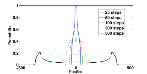
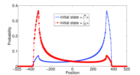
Figure 1: (color online) Probability distribution of 51 particles initially located individually at positions $j=-25$ to $j=+25$ after the quantum walk evolution using using the Hadamard operator $B(\pi/4)$ as the quantum coin. (a) The initial state of all the particles is $\frac{1}{\sqrt{2}}(|\downarrow\rangle+i|\uparrow\rangle)$ and evolves in position space. The spread of the distribution with an increasing number of steps is clearly visible. (b) Initially all particles are either in state $|\downarrow\rangle$ or state $|\uparrow\rangle$ and subsequently subjected to the quantum walk of 500 steps. For all the particle in the initial state $|\downarrow\rangle$, the distribution with peak on the left is obtained and for all the particle in the initial state $|\uparrow\rangle$, the distribution with peak on the right is obtained.

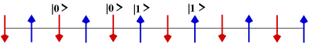
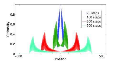
Figure 2: (color online)(a) The initial state has an antiferromagnetic ordering with neighboring particles being in different internal states. (b) Probability distribution of 51 particles, initially in the state shown in (a) with one particle in each position ranging from $j=-25$ to $j=+25$, after a quantum walk of different number of steps using the Hadamard operator $B(\pi/4)$ as the quantum coin. Lower parts in the left (right) of the distribution are due to the low contribution of state $|\downarrow\rangle$ ( $|\uparrow\rangle$) from the particle initially in state $|\uparrow\rangle$ ($|\downarrow\rangle$).

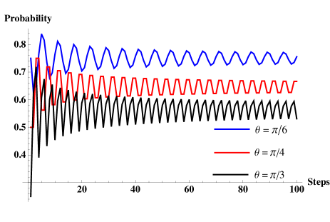
Figure 3: (color online) Probability of finding a particle in state $|\downarrow\rangle$ of a single-particle walk with increasing number of steps if the particle was initially in state $|\downarrow\rangle$. For small values of $\theta$ the probability of finding the particle in state $|\downarrow\rangle$ is larger than for larger value of $\theta$.

Though the evolution of distinguishable particles does not involve many-particle interference effect, the collective behavior of the single particle interference effects can reveal interesting features of the systems dynamics. Such systems can be approximately realized in cold, but thermal samples of neutral atomic gases in optical lattices KFC09 , which can be engineered to minimize the atom-atom interaction and dynamically control the atom transport MGW03 ; DDL03 ; Jak04 . Therefore, they have been suggested for observation of quantum phase transitions CL08 or for generation and control over spatial entanglement between different lattice sites GC10 . Another interesting question is the exploration of the meeting probabilities and meting times of many-particles at pre-defined positions (see Ref. SKJ06 for two particle meeting probabilities).

In this section we will define the non-interacting distinguishable many-particle quantum walk and discuss some of the interesting outcomes from the collective evolution. To define a simple form of distinguishable many-particle quantum walk in one-dimension, we will consider a system of $M$ non-interacting particles, where initially exactly one particle occupies a lattice site and every particle has its own coin and position Hilbert space, $\mathcal{H}=\left(\mathcal{H}_{c}\otimes\mathcal{H}_{p}\right)^{\otimes M}$. If the number of particles is odd , the initial state can be written as

$$|\Psi_{ins}^{M}\rangle=\bigotimes_{j=-\frac{M-1}{2}}^{j=\frac{M-1}{2}}\left[\left(\frac{|\downarrow\rangle+i|\uparrow\rangle}{\sqrt{2}}\right)\otimes|\psi_{j}\rangle\right],$$ (6)

which, after $t$ steps, will evolve into

$$|\Psi_{t}^{M}\rangle=[W(\theta)^{\otimes M}]^{t}\bigotimes_{j=-\frac{M-1}{2}}^{j=\frac{M-1}{2}}\left[\left(\frac{|\downarrow\rangle+i|\uparrow\rangle}{\sqrt{2}}\right)\otimes|\psi_{j}\rangle\right].$$ (7)

Here $W(\theta)^{\otimes M}$ is the evolution operator for each step of the walk, which will evolve each particle into the superposition of its neighboring positions, establishing the quantum correlation between the particle and the position space. After $t$ steps, these correlations overlap resulting in,

$$[W(\theta)^{\otimes M}]^{t}|\Psi_{in}^{M}\rangle\propto\bigotimes_{j=-\frac{M-1}{2}}^{\frac{M-1}{2}}[\mathcal{A}_{j-t}|\downarrow\rangle\otimes|\psi_{j-t}\rangle$$

$$+\mathcal{A}_{j-t+1}|\downarrow\rangle\otimes|\psi_{j-t+1}\rangle+......+\mathcal{A}_{j+t}|\downarrow\rangle\otimes|\psi_{j+t}\rangle$$

$$+\mathcal{B}_{j-t}|\uparrow\rangle\otimes|\psi_{j-t}\rangle+......+\mathcal{B}_{j+t})|\uparrow\rangle\otimes|\psi_{j+t}\rangle],$$ (8)

which can be written as

$$[W(\theta)^{\otimes M}]^{t}|\Psi_{in}^{M}\rangle\propto$$

$$\bigotimes_{j=-\frac{M-1}{2}}^{\frac{M-1}{2}}\left(\sum\limits_{x=j-t}^{j+t}[\mathcal{A}_{x}^{j}|\downarrow\rangle+\mathcal{B}_{x}^{j}|\uparrow\rangle]\otimes|\psi_{x}\rangle\right).$$ (9)

Here $\mathcal{A}_{x}^{j}$ and $\mathcal{B}_{x}^{j}$ are the probability amplitudes of the state $|\downarrow\rangle$ and $|\uparrow\rangle$ of each of the particles initially at position $j$ at the new position $x$, which range from $(j-t)$ to $(j+t)$ after the $t$ step walk.

The probability distribution after $t$ steps is given by the sum of the probabilities at a given lattice site of each particle $k$

$$P(j,t)=\sum_{k=1}^{M}P_{k}(j,t)$$ (10)

and the effective probability distribution for different numbers of steps is shown in Fig. 1. As expected, after $t$ steps of the quantum walk, the $M$ particles are spread between $(M-t)$ and $(M+t)$. In Fig. 1 the asymmetric probability distributions resulting from all particles being initially in state $|\downarrow\rangle$ or $|\uparrow\rangle$ after 500 steps are shown. From Fig. 1, and 1, it is clearly evident that when $t\gg M$ the probability distribution profile of $M$ particles resembles the single-particle profile. From earlier studies of single-particle quantum walks of $t$ steps on a particle initially at position $j=0$ using $B_{\theta}$ as the quantum coin it is known that the probability distribution spreads over the interval $(-t\cos(\theta),t\cos(\theta))$ in position space and decays quickly outside this region NV01 ; CSL08 . For an $M$ particle system the peak of the effective probability distribution is given by contributions from the probability of all $M$ particles and therefore located at $\mp[t\cos(\theta)-M/2]$.

Apart from all particles being initially in the symmetric superposition state of $|\downarrow\rangle$ and $|\uparrow\rangle$ (see Eq.(6)), one can also consider a situation of antiferromagnetic ordering (see Fig. 2), where two neighboring particles are in opposite states. In Fig. 2 we show the final probability distribution for this situation after a different number of steps. Though each particle undergoes an asymmetric evolution with the states $|\downarrow\rangle$ moving left and the states $|\uparrow\rangle$ moving right, the collective distribution is symmetric due to equal number of particles initially in both states.

Many-particle quantum walks of particles initially in antiferromagnetic order or in a completely randomized initial state are very useful for separating different basis states of the particles in position space and grouping them together. Using a different angle $\theta$ in the quantum coin operation one can find different outcomes for the probabilities of basis states grouped after the evolution of the quantum walk. To demonstrate this we will consider the examples of a single-particle initially in one of the basis state.

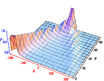
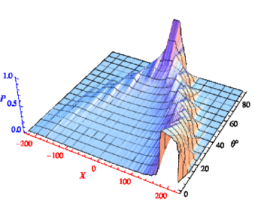
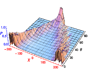
Figure 4: (color online) Probability distribution of 51 particles after 200 steps for different values of $\theta$. The states $|\downarrow\rangle$ walk to the left and the states $|\uparrow\rangle$ to the right. In (a) the initial state of all particle was $|\downarrow\rangle$ and in (b) the initial state of all particle was $|\uparrow\rangle$. In (c) the initial state of each particle is randomly choose from $|\downarrow\rangle$ and $|\uparrow\rangle$.

A quantum walk of a single particle initially in state $|\downarrow\rangle$ (or equivalently $|\uparrow\rangle$) using a Hadamard coin ($\theta=\pi/4$) results in constructive interference towards the left (right) of the origin and therefore localizes all particles with high probability on the left (right) of the origin. To understand this, let us look at the analytic form of the evolution after $t$ steps using $B(\theta)$ as coin operator. The state after $t$ steps can be written as

$$W(\theta)^{t}|\Psi_{ins}\rangle=|\Psi(t)\rangle=\sum_{j=-t}^{t}(\mathcal{A}_{j,t}|\downarrow\rangle|\psi_{j}\rangle+\mathcal{B}_{j,t}|\uparrow\rangle|\psi_{j}\rangle)$$ (11)

where $\mathcal{A}_{j,t}$ and $\mathcal{B}_{j,t}$ are given by the coupled iterative relations

$$\mathcal{A}_{j,t}=\cos(\theta)\mathcal{A}_{j+1,t-1}+\sin(\theta)\mathcal{B}_{j+1,t-1}$$ (12a)

$$\mathcal{B}_{j,t}=-\cos(\theta)\mathcal{B}_{j-1,t-1}+\sin(\theta)\mathcal{A}_{j-1,t-1}.$$ (12b)

Straightforward algebra allows to decouple these equations at the price of a time-dependence on the previous two steps

$$\mathcal{A}_{j,t}=\cos(\theta)\left(\mathcal{A}_{j+1,t-1}-\mathcal{A}_{j-1,t-1}\right)-\mathcal{A}_{j,t-2}$$ (13a)

$$\mathcal{B}_{j,t}=\cos(\theta)\left(\mathcal{B}_{j+1,t-1}-\mathcal{B}_{j-1,t-1}\right)-\mathcal{B}_{j,t-2}.$$ (13b)

By repeating this process of substitution one can find an expression linking $\mathcal{A}_{j,t}$ and $\mathcal{B}_{j,t}$ to the amplitude of the initial state of the particle and the angle, $\theta$, of the coin operation. Therefore, the expression for the total probability of finding the particle in state $|\downarrow\rangle$ and $|\uparrow\rangle$ after time $t$ is

$$P_{|\downarrow\rangle}(t)=\sum_{j}|\mathcal{A}_{j,t}|^{2}$$ (14a)

$$P_{|\uparrow\rangle}(t)=\sum_{j}|\mathcal{B}_{j,t}|^{2}$$ (14b)

To obtain a spatially symmetric probability distribution for a particle initially in symmetric superposition state, the walk should be invariant under an exchange of $|0\rangle\leftrightarrow|1\rangle$, and hence should evolve $\mathcal{A}_{j,t}$ and $\mathcal{B}_{j,t}$ alike (as, for example, the Hadamard walk does KRS03 ). From the above analysis we see that $\mathcal{A}_{j,t}$ and $\mathcal{B}_{j,t}$ are symmetric to each other and evolve alike for all value of $\theta$ only when the initial state of the particle is a symmetric superposition state. When the initial state is $|\downarrow\rangle$, the walk will evolves with constructive interference towards left and destructive interference to the right, (exact form depending on the value of $\theta$) and vice versa when the initial state is $|\uparrow\rangle$. The associated probability amplitudes oscillate strongly between the left and the right hand side for small numbers of steps and stabilize for longer times. This can be seen in Fig. 3 and also directly from Eq. (13) when realizing that the amplitude at each position oscillates and the range of oscillation reduces as the amplitude at each position decreases over time Rom10 .

For a particle initially in state $|\downarrow\rangle$ a smaller value of $\theta$ returns a high probability of finding the particle in state $|\downarrow\rangle$ but if the initial state is $|\uparrow\rangle$ the probability of finding the particle in $|\downarrow\rangle$ will be very low. We should also note that a small probability of state $|\uparrow\rangle$ ($|\downarrow\rangle$) is present along with the state $|\downarrow\rangle$ ($|\uparrow\rangle$) to the left (right) of the origin but that will not alter the trend. From the above analysis we can conclude that an initially randomized many-particle state can be efficiently sorted in position space with respect to its basis states. This in turn allows to create an ordered state with high probability.

To demonstrate this we show in Fig. 4 the probability distribution for different values of $\theta$ for a sample of 51 particles after 200 steps when the initial state of all the particles was $|\downarrow\rangle$ and Fig. 4 shows the same for an initial state of $|\uparrow\rangle$. A strong asymmetry is visible for both cases. In contrast, the probability distribution shown in Fig. 4 assumes that the initial state of each particle was randomly chosen from $|\downarrow\rangle$ and $|\uparrow\rangle$ and the anisotropy in the final distribution vanishes. From Figs. 4 and (4) one can also see that for increasing $\theta$ the probability distribution widens and its maximum amplitude decreases.

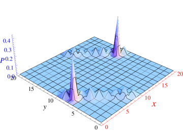
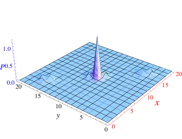
Figure 5: (color online) Probability distribution of two distinguishable particles on a two-dimensional lattice using $B(\pi/4)$ as quantum coin operation. (a) Joint probability distribution of two particles staring at $(0,0)$ and $(20,20)$ with initial states $|\downarrow\rangle$ after 10 steps. (b) Localization of two-particle probability distribution at the center of the lattice after a one time bit-flip operation on both particles at $t=j/2$ was introduced.

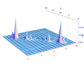
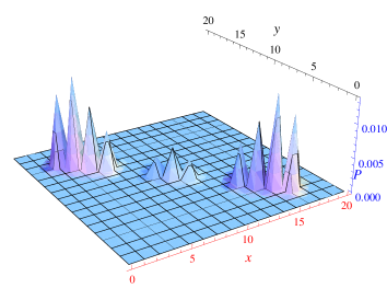
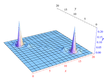
Figure 6: (color online) Quantum walk on a two-dimensional lattice for two indistinguishable bosons initially at $(0,0)$ and $(20,20)$ in $|\downarrow\downarrow\rangle$ and interacting via $\sigma_{x}$ after 20 steps using $B(\pi/4)$ as the quantum coin operation. The probabilities for finding the particles in the state (a) $|\downarrow\downarrow\rangle$ (b) $|\uparrow\uparrow\rangle$ and (c) $|\downarrow\uparrow\rangle$ are shown at $t=20$. The relative height of the final distributions however can be shown to depend on the initial state.

III Joint probability of two-particle quantum walk

Two-particle quantum walks have been studied from various perspectives OPS06 ; GFZ10 ; SBK11 ; BW11 and first experimental implementations have recently been reported ZKG10 ; PLM10 . Here we will discuss the probability distribution of a quantum walk using two distinguishable particles on a two-dimensional lattice and present a protocol to increase the meeting probability of the two particle at a particular lattice after a particular time. We then compare this to the quantum walk evolution of two indistinguishable particles which only interact at the end of a certain number of steps.

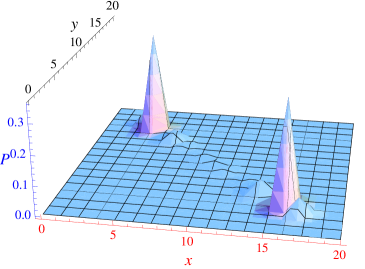
Figure 7: (color online) Probability distribution of finding the two fermions staring at $(0,0)$ and $(20,20)$ with initial states $|\downarrow\rangle$ and interacting with $\sigma_{x}$ after 20 steps of quantum walk on a two-dimensional lattice using $B(\pi/4)$ as quantum coin operation. The state $|\downarrow\uparrow\rangle$ is the only possible state for fermions.

To define a two-particle quantum walk we will consider a two-dimensional square lattice and label the two axis as $X$ and $Y$ such that $(x,y)$ represent a position on the lattice. We will consider two particles initially in state $|\downarrow\rangle$ at diagonally opposite points $(0,0)$ and $(j,j)$,

$$|\Psi_{ins}^{2}\rangle=\left[|\downarrow\rangle\otimes|\psi_{0,0}\rangle\right]\otimes\left[|\downarrow\rangle\otimes|\psi_{j,j}\rangle\right],$$ (15)

where $j$ is the length of the lattice, which has $j\times j$ positions. The shift operator for the quantum walk evolution is defined separately for both particles in such a way that they evolve towards each other,

$$S_{1}\equiv\sum_{x,y}[|\downarrow\rangle\langle\downarrow|\otimes|\psi_{x+1,y}\rangle\langle\psi_{x,y}|$$

$$+|\uparrow\rangle\langle\uparrow|\otimes|\psi_{x,y+1}\rangle\langle\psi_{x,y}|]$$

$$S_{2}\equiv\sum_{x,y}[|\downarrow\rangle\langle\downarrow|\otimes|\psi_{x-1,y}\rangle\langle\psi_{x,y}|$$

$$+|\uparrow\rangle\langle\uparrow|\otimes|\psi_{x,y-1}\rangle\langle\psi_{x,y}|].$$ (16)

Each step of the evolution can be implemented by $W_{2}(\theta)=[B(\theta)\otimes S_{1}]\otimes[B(\theta)\otimes S_{2}]$ and after $t$ steps the state is given by

$$[W_{2}(\theta)]^{t}|\Psi_{ins}^{2}\rangle=\left\{[B(\theta)\otimes S_{1}]\otimes[B(\theta)\otimes S_{2}]\right\}^{t}$$

$$\times\left\{[|\downarrow\rangle\otimes|\psi_{0,0}\rangle]\otimes[|\downarrow\rangle\otimes|\psi_{j,j}\rangle]\right\}.$$ (17)

The two particles meet each other for the first time after $t=j$ steps and the meeting probability at each position is different for the distinguishable and indistinguishable case.

Two distinguishable particles: In this case the joint probability of the two particles at each position at the time of meeting each other is the sum of the probabilities of both individual particle. In Fig. 5 we show this distribution for both particles after $t=j/2=10$ steps on a $20\times 20$ lattice. The first time the two distributions overlap is at $t=20$ where they spread along the diagonal of the lattice (not shown). If, however, we introduce a one time bit-flip operation, $\sigma_{x}$ at t=j/2=10,

$$[W(\theta)^{\otimes 2}]^{j/2}[\sigma_{x}\otimes\sigma_{x}][W(\theta)^{\otimes 2}]^{j/2}|\Psi_{ins}^{2}\rangle$$ (18)

one can see from Fig. 5 that the evolution can be reversed, which leads to localization of both the particles in the center of the lattice at time $t=j$ with a good probability.

Two indistinguishable particle: If the two particles are indistinguishable, their probability distributions interfere when they overlap at the same position in the lattice. For bosons the allowed states at each position in the lattice are $|\downarrow\downarrow\rangle$, $|\uparrow\uparrow\rangle$ or $|\downarrow\uparrow\rangle\equiv|\downarrow\uparrow\rangle$, whereas for fermions these are restricted to $|\downarrow\uparrow\rangle\equiv|\downarrow\uparrow\rangle$. The probabilities for these states to be obtained at each position at time $t$ are then given for bosons as

$$P^{j}_{|\downarrow\downarrow\rangle}=\frac{|\mathcal{A}^{a}_{j,t}|^{2}\cdot|\mathcal{A}^{b}_{j,t}|^{2}}{\sum_{j}[|\mathcal{A}^{a}_{j,t}|^{2}\cdot|\mathcal{A}^{b}_{j,t}|^{2}+|\mathcal{B}^{a}_{j,t}|^{2}\cdot|\mathcal{B}^{b}_{j,t}|^{2}+|\mathcal{A}^{a}_{j,t}|^{2}\cdot|\mathcal{B}^{b}_{j,t}|^{2}+\mathcal{A}^{b}_{j,t}|^{2}\cdot|\mathcal{B}^{a}_{j,t}|^{2}]}$$ (19a)

$$P^{j}_{|\uparrow\uparrow\rangle}=\frac{|\mathcal{B}^{a}_{j,t}|^{2}\cdot|\mathcal{B}^{b}_{j,t}|^{2}}{\sum_{j}[|\mathcal{A}^{a}_{j,t}|^{2}\cdot|\mathcal{A}^{b}_{j,t}|^{2}+|\mathcal{B}^{a}_{j,t}|^{2}\cdot|\mathcal{B}^{b}_{j,t}|^{2}+|\mathcal{A}^{a}_{j,t}|^{2}\cdot|\mathcal{B}^{b}_{j,t}|^{2}+\mathcal{A}^{b}_{j,t}|^{2}\cdot|\mathcal{B}^{a}_{j,t}|^{2}]}$$ (19b)

$$P^{j}_{|\uparrow\downarrow\rangle}=\frac{|\mathcal{A}^{a}_{j,t}|^{2}\cdot|\mathcal{B}^{b}_{j,t}|^{2}+|\mathcal{A}^{b}_{j,t}|^{2}\cdot|\mathcal{B}^{a}_{j,t}|^{2}}{\sum_{j}[|\mathcal{A}^{a}_{j,t}|^{2}\cdot|\mathcal{A}^{b}_{j,t}|^{2}+|\mathcal{B}^{a}_{j,t}|^{2}\cdot|\mathcal{B}^{b}_{j,t}|^{2}+|\mathcal{A}^{a}_{j,t}|^{2}\cdot|\mathcal{B}^{b}_{j,t}|^{2}+\mathcal{A}^{b}_{j,t}|^{2}\cdot|\mathcal{B}^{a}_{j,t}|^{2}]}.$$ (19c)

Here $\mathcal{A}^{a}$ and $\mathcal{A}^{b}$ are the amplitudes of the particles $a$ and $b$ to be in state $|\downarrow\rangle$, and $\mathcal{B}^{a}$ and $\mathcal{B}^{b}$ are the amplitudes to be in the state $|\uparrow\rangle$. We show these probabilities two particles initially at $(0,0)$ and $(20,20)$ and meeting after evolving for 20 steps of walk using Eq. (III) in Fig. 6,(b) and (c).

If the particles are fermions the probability of finding the two-particle in the only possible state at each positions is

$$P^{j}_{|\downarrow\uparrow\rangle}=\frac{\|\mathcal{A}^{a}_{j,t}|^{2}\cdot|\mathcal{B}^{b}_{j,t}|^{2}+|\mathcal{A}^{b}_{j,t}|^{2}\cdot|\mathcal{B}^{a}_{j,t}|^{2}}{\sum_{j}[\|\mathcal{A}^{a}_{j,t}|^{2}\cdot|\mathcal{B}^{b}_{j,t}|^{2}+|\mathcal{A}^{b}_{j,t}|^{2}\cdot|\mathcal{B}^{a}_{j,t}|^{2}]},$$ (20)

which is shown in Fig. 7 for the same parameters as in the bosonic case above. The difference to the bosonic case is clearly visible. Using different initial states of the particle or different coin operations during the evolution will of course alter the probability distribution. Introducing a one time bit-flip operation half way through the evolution for indistinguishable particles as we did for distinguishable particle will lead to localization of the join probability at the center (not shown).

From this one can see that even a one time particle-particle interaction in an indistinguishable many-particle quantum walk can result in different probability distributions which might be useful for applications in quantum information and other fundamental quantum mechanical experiments. With the possibility of increasing the number of steps, the number of particles and the number of time the particle-particle interaction is introduced, the evolution gets even more interesting and complicated, but becomes computationally difficult. Recently,for the case of two atoms in an optical lattice performing a quantum walk with interactions via cold collisions the appearance of a bound state has been predicted AAM11 , which gives scope for further exploration of the dynamics using our approach for many-particle system by introducing interactions at regular intervals.

IV Conclusion

We have presented a number examples of quantum walk dynamics of many-particle system with different initial states of the particles. Though the distinguishable many-particle quantum walk dynamics does not involve many-particle interference during the evolution we have shown that it can be effectively used to separate the eigenstates of the particles position space and group them together. We have also presented an example of two-particle quantum walk dynamics with defined interaction that can lead to localization of two distinguishable particles at the center if they start their walk from opposite ends of the lattice. Extending this scheme to indistinguishable boson and fermion pairs results in the different probabilities for finding the two particles in the allowed combination of states. Recent experimental developments in implementing quantum walks and using quantum walk models to simulate and understand some of the dynamics process in nature suggests that collective dynamics of many-particle system will very useful for further studies.

References

- (1) G. V. Riazanov, Sov. Phys. JETP 6 1107 (1958).
- (2) R. P. Feynman and A.R. Hibbs, Quantum Mechanics and Path Integrals (McGraw-Hill, New York, 1965).
- (3) Y. Aharonov, L. Davidovich and N. Zagury, Phys. Rev. A 48, 1687, (1993).
- (4) D. A. Meyer, J. Stat. Phys. 85, 551 (1996).
- (5) E. Farhi and S. Gutmann, Phys.Rev. A 58, 915 (1998).
- (6) A. Ambainis, E. Bach, A. Nayak, A. Vishwanath and J. Watrous, Proceeding of the 33rd ACM Symposium on Theory of Computing (ACM Press, New York, 2001), p.60.
- (7) A. Nayak and A. Vishwanath, DIMACS Technical Report, No. 2000-43 (2001) ; arXiv:quant-ph/0010117.
- (8) A. Ambainis, Int. Journal of Quantum Information, 1, No.4, 507-518 (2003).
- (9) A. M. Childs, R. Cleve, E. Deotto, E. Farhi, S. Gutmann and D. A. Spielman, in Proceedings of the 35th ACM Symposium on Theory of Computing (ACM Press, New York, 2003), p.59.
- (10) N. Shenvi, J. Kempe and K. Birgitta Whaley, Phys. Rev. A 67, 052307, (2003).
- (11) A. Ambainis, J. Kempe, and A. Rivosh, Proceedings of ACM-SIAM Symp. on Discrete Algorithms (SODA), (AMC Press, New York, 2005), pp.1099-1108.
- (12) C. M. Chandrashekar and R. Laflamme, Phys. Rev. A 78, 022314 (2008).
- (13) T. Oka, N. Konno, R. Arita, and H. Aoki, Phys. Rev. Lett. 94, 100602 (2005).
- (14) G. S. Engel et. al., Nature 446, 782-786 (2007).
- (15) M. Mohseni, P. Rebentrost, S. Lloyd, A. Aspuru-Guzik, J. Chem. Phys. 129, 174106 (2008).
- (16) C. M. Chandrashekar, Sandeep K Goyal, and Subhashish Banerjee, arXiv:1005.3785 (2010).
- (17) T. Kitagawa, M. S. Rudner, E. Berg, and E. Demler, Phys. Rev. A 82, 033429 (2010).
- (18) J. Du, H. Li, X. Xu, M. Shi, J. Wu, X. Zhou, and R. Han, Phys. Rev. A 67, 042316 (2003)
- (19) C. A. Ryan, M. Laforest, J. C. Boileau, and R. Laflamme, Phys. Rev. A 72, 062317 (2005).
- (20) H. B. Perets, Y. Lahini, F. Pozzi, M. Sorel, R. Morandotti, and Y. Silberberg, Phys. Rev. Lett. 100, 170506 (2008).
- (21) H. Schmitz, R. Matjeschk, Ch. Schneider, J. Glueckert, M. Enderlein, T. Huber, and T. Schaetz, Phys. Rev. Lett. 103, 090504 (2009).
- (22) F. Zahringer, G. Kirchmair, R. Gerritsma, E. Solano, R. Blatt, and C. F. Roos, Phys. Rev. Lett. 104, 100503 (2010).
- (23) K. Karski, L. Foster, J.-M. Choi, A. Steffen, W. Alt, D. Meschede, and A. Widera, Science 325, 174 (2009).
- (24) A. Schreiber, K. N. Cassemiro, V. Potocek, A. Gabris, P. Mosley, E. Andersson, I. Jex, and Ch. Silberhorn, Phys. Rev. Lett., 104, 05502 (2010).
- (25) M. A. Broome, A. Fedrizzi, B. P. Lanyon, I. Kassal, A. Aspuru-Guzik, and A. G. White. Phys. Rev. Lett. 104, 153602 (2010).
- (26) Alberto Peruzzo, Mirko Lobino, Jonathan C. F. Matthews, Nobuyuki Matsuda, Alberto Politi, Konstantinos Poulios, Xiao-Qi Zhou, Yoav Lahini, Nur Ismail, Kerstin Wörhoff4, Yaron Bromberg, Yaron Silberberg, Mark G. Thompson and Jeremy L. OBrien, Science, 329, 1500-1503 (2010).
- (27) J. O. Owens, M. A. Broome, D. N. Biggerstaff, M. E. Goggin, A. Fedrizzi, T. Linjordet, M. Ams, G. D. Marshall, J. Twamley, M. J. Withford and A. G. White, New J. Phys. 13, 075003 (2011).
- (28) N. Konno, Quantum Information Processing, 1, Issue 5, pp.345-354 (2002).
- (29) C. M. Chandrashekar, R. Srikanth, and R. Laflamme, Phys. Rev. A 77, 032326 (2008).
- (30) Klaus Mayer, Malte C. Tichy, Florian Mintert, Thomas Konrad, and Andreas Buchleitner, Phys. Rev. A 83, 062307 (2011).
- (31) Peter. P. Rohde, Andreas Schreiber, Martin Stefanak, Igor Jex and Christine Silberhorn, New J. Phys. 13, 013001 (2011).
- (32) Sandeep K Goyal and C. M. Chandrashekar, J. Phys. A: Math. Theor. 43, 235303 (2010).
- (33) O. Mandel, M. Greiner, A. Widera, T. Rom, T.W. Hänsch, and I. Bloch, Phys. Rev. Lett. 91, 010407 (2003).
- (34) L.-M. Duan, E. Demler, M. D. Lukin, Phys. Rev. Lett. 91, 090402 (2003).
- (35) D. Jaksch, Contemporary Physics, 45 No. 5, 367-381 (2004).
- (36) M. Stefanak, T. Kiss, I. Jex, and B. Mohring, J. Phys. A : Math. Gen. 39 14965-14983 (2006).
- (37) P. L. Knight, E. Roldan, and J. E. Sipe. Quantum walk on the line as an interference phenomenon. Phys. Rev. A, 68 020301(R) (2003).
- (38) Y. Omar, N. Paunkovic, L. Sheridan, and S. Bose, Phys. Rev. A 74 042304 (2006).
- (39) John King Gamble, Mark Friesen, Dong Zhou, Robert Joynt, and S. N. Coppersmith, Phys. Rev. A 81 052313 (2010).
- (40) M. Stefanak , S. M. Barnett, B. Kollar, T. Kiss and I. Jex, New Journal of Physics 13 033029 (2011).
- (41) Scott D. Berry and Jingbo B. Wang, Phys. Rev. A 83 042317 (2011).
- (42) Alejandro Romanelli, Phys. Rev. A, 81 062349 (2011).
- (43) Andre Ahlbrecht, Andrea Alberti, Dieter Meschede, Volkher B. Scholz, Albert H. Werner, and Reinhard F. Werner, arXiv:1105.1051v1 (2011).