FERMILAB-PUB-12/062-E
The D0 Collaboration111with visitors from aAugustana College, Sioux Falls, SD, USA, bThe University of Liverpool, Liverpool, UK, cUPIITA-IPN, Mexico City, Mexico, dDESY, Hamburg, Germany, ,eSLAC, Menlo Park, CA, USA, fUniversity College London, London, UK, gCentro de Investigacion en Computacion - IPN, Mexico City, Mexico, hECFM, Universidad Autonoma de Sinaloa, Culiacán, Mexico and iUniversidade Estadual Paulista, São Paulo, Brazil. ‡Deceased.
Search for associated production in collisions at
Abstract
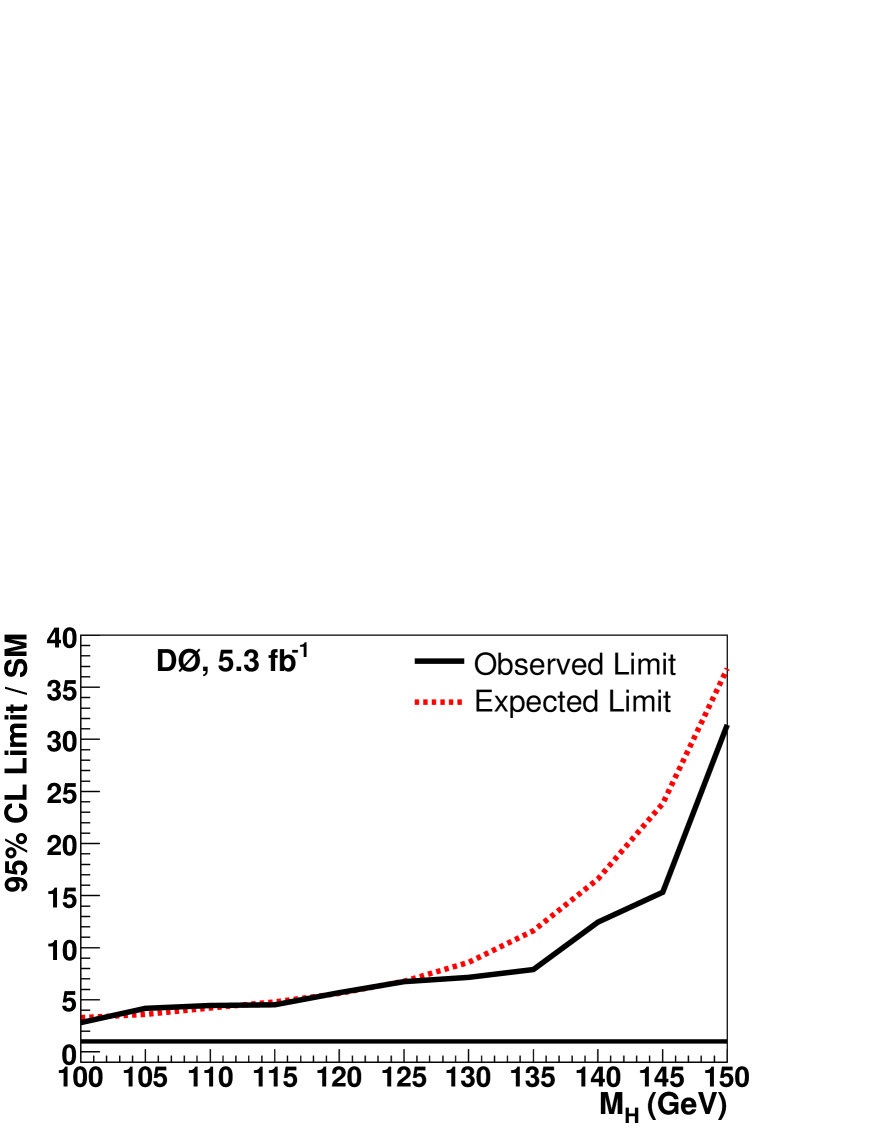
This report describes a search for associated production of and Higgs bosons based on data corresponding to an integrated luminosity of collected with the D0 detector at the Fermilab Tevatron Collider. Events containing a candidate (with corresponding to or ) are selected in association with two or three reconstructed jets. One or two of the jets are required to be consistent with having evolved from a quark. A multivariate discriminant technique is used to improve the separation of signal and backgrounds. Expected and observed upper limits are obtained for the product of the production cross section and branching ratios and reported in terms of ratios relative to the prediction of the standard model as a function of the mass of the Higgs boson (). The observed and expected 95% C.L. upper limits obtained for an assumed are, respectively, factors of 4.5 and 4.8 larger than the value predicted by the standard model.
pacs:
14.80.Bn,13.85.RmI Introduction
In the standard model (SM) of particle physics, the masses of the weakly interacting and gauge bosons are accommodated through the process of electroweak symmetry breaking, and the masses of fermions through their Yukawa couplings to the Higgs field. The search for the Higgs boson, whose mass is not predicted by the SM, is a test of this hypothesis and is a major component of the experimental programs at particle colliders. At the Fermilab Tevatron Collider, this search is carried out using multiple statistically independent search samples, each sensitive to different Higgs boson production processes and decay channels, providing increased sensitivity in the search for direct evidence for this SM mechanism combTEV ; combD0 .
This paper presents an extended description of the previously reported search WH for SM Higgs boson production through the process , in which a Higgs boson is produced in association with a boson. The search is based on data corresponding to an integrated luminosity collected with the D0 detector at the Fermilab Tevatron Collider with a center-of-mass energy . The events are required to contain a or candidate, thereby suppressing background from inclusive -jet production processes, and enhancing sensitivity to signal by several orders of magnitude. The event selection is also sensitive to events with decay into electrons or muons. The events are required to contain a candidate because of large branching fraction for this decay in the region considered here (). The experimental signature is therefore a single isolated lepton, an imbalance in the measured transverse energy (), and either two or three jets, at least one of which is consistent with having been initiated by a quark. The three-jet sample is included to provide additional sensitivity for events containing gluon radiation from the initial or final-state particles of the hard collision. The data are examined in separate search samples of different sensitivity and a multivariate random forest technique RF1 ; RF2 is applied to each sample, further enhancing sensitivity to signal.
Direct searches for the process at the CERN Collider (LEP) experiments set the SM Higgs mass to CERN . In addition, a fit to electroweak precision measurements of the masses of the boson and the top quark from both Tevatron and LEP experiments leads to an upper limit of for SM Higgs production at the 95% C.L. EWFIT . Both the CDF and D0 Collaborations have extensively investigated the associated production mechanism D0WH1 ; D0WH2 ; D0WH3 ; CDFWH1 ; CDFWH2 ; CDFWH3 , and a region at larger has also been excluded at 95% C.L. by direct searches for decays Exclude . Results from the CERN Large Hadron Collider (LHC) Collaborations ref:ATLAS ; ref:CMS also exclude regions at higher and indicate that the most interesting region for the search for the SM Higgs boson is the one where the sensitivity of the search discussed in this article is maximal. The analysis presented here is expected to be a highly sensitive channel in the mass range , and complements searches at the LHC which rely primarily on different SM Higgs production and decay mechanisms in this mass range.
II The D0 Detector
The main components of the D0 detector used in this investigation are the tracking detectors, calorimeters, muon detectors, and the luminosity system. Protons and antiprotons interact close to the origin of the D0 detector coordinate system, which is at the center of the detector. A right-handed Cartesian coordinate system is used with the positive axis pointing along the nominal direction of the incoming proton beam (the positive axis points toward the top of the detector) and the pseudorapidity variable, defined as , where is the polar angle in the corresponding spherical polar coordinate system. The kinematic properties of particles and jets are measured with respect to the reconstructed collision vertex. More details on D0 construction and component design are available in Refs. d0det_run2 ; d0det_run1 . Upgrades to the tracking and trigger systems were installed during the summer of 2006 and the data samples collected prior to and after this upgrade are referred to as pre- and post-upgrade samples in the following.
II.1 Tracking Detectors
The D0 tracking system surrounds the interaction point and consists of an inner silicon microstrip tracker (SMT) followed by an outer central scintillating fiber tracker (CFT). Both the SMT and CFT are situated within a 2 T magnetic field provided by a superconducting solenoidal coil surrounding the entire tracking system.
The silicon microstrip tracker is used for tracking charged particles and reconstructing interaction and decay vertices. In the central region there are six barrel sections each comprising four detector layers. The barrel sections are interspersed and capped with disks composed of 12 double-sided silicon wedge detectors. The first and second detector layers of each barrel contain 12 silicon modules and 24 modules are installed in the third and fourth detector layers. An additional inner layer was added to the silicon tracker system in 2006 smt_layer . In the high region on either side of the three disk-barrel assemblies there are three further radial disk sections (F-disks), and in the far-forward region, large-diameter disks (H-disks) provide tracking at larger . The tracks of particles with are measured using the CFT and the barrel and F-disk sections of the SMT, whereas tracks for particles at larger are reconstructed using the the F- and H-disks.
The CFT comprises scintillating fibers ( in diameter) mounted on eight concentric support cylinders. The cylinders occupy the radial space from 20 to 52 cm from the center of the beam pipe. The two innermost cylinders are long whereas the outer six cylinders are long. The outer cylinder provides tracking coverage extending to .
II.2 Calorimeters
The D0 calorimeter system is used to measure energies as well as to identify electrons, photons, and jets. The calorimeter also helps to identify muons and provides a measure of the in events. The central calorimeter (CC) and the two end calorimeters (EC) are contained within three individual cryostats located outside of the superconducting solenoid. The central calorimeter covers detector pseudorapidities and the end calorimeters extend the range to . The active material in each calorimeter section is liquid argon. Extending radially outwards from the detector center, the calorimeters are subdivided into electromagnetic (EM), fine hadronic, and coarse hadronic (CH) sections. The absorber material of the EM sections is uranium, whereas for the fine hadronic sections a uranium-niobium alloy is used. The CH absorbers are made of copper in the CC region and stainless steel in the EC region. To improve measurements in the intercryostat regions, plastic-scintillator detectors and “massless gap” detectors are used to sample showers between cryostats, enhancing calorimeter coverage in the region .
II.3 Muon Detectors
The muon detector system d0muo_run2 consists of a central muon detector system covering the range and a forward muon system that covers the region . The central muon system comprises aluminum proportional drift chambers whereas aluminum mini drift tubes are used in the forward system. Scintillation counters are included for triggering purposes, and 1.8 T toroidal magnets make it possible to determine muon momenta and perform tracking measurements based on the muon system alone.
The proportional drift chambers are arranged in three layers, one of which (A layer) is located within the toroid, with the remaining two (B and C) layers located beyond the toroid, with the C layer radially furthest from the interaction point. In the central muon system, the B and C layers have three planes of drift cells. The A layer has four planes, except at the support structure at the bottom of the detector, where the A layer has three planes of cells. In the forward region, mini drift tubes are arranged in eight octants with four planes in the A layer while the B and C layers each have three planes.
II.4 Luminosity System
The D0 luminosity system is used to determine the instantaneous luminosity and also to measure beam-halo rates. The system is composed of two disks of scintillating tile detectors that are positioned in front of the ECs on both sides of the D0 detector at . Each of the disks consists of 24 plastic scintillation counters that cover pseudorapidity regions . The total integrated luminosity () is determined via the average instantaneous number of observed inelastic collisions (), according to , where is the frequency of Tevatron bunch crossings, and is the effective inelastic production cross section inelas within the luminosity system acceptance, after taking into account beam-halo events and multiple collisions within a single beam crossing. In practice, is calculated by inverting the Poisson probability of observing no hits in either of the two disks lumi_ID .
III Triggering
The D0 trigger system has three levels referred to as L1, L2, and L3. Each consecutive level receives a lower rate of events for further examination. The L2 software-based algorithms refine the L1 information they receive and the L3 software-based algorithms then run simplified versions of offline identification algorithms based on the full detector readout.
The candidates of this search are collected using the logical OR Boole of different triggers requiring a candidate electromagnetic object. The L1 electron triggers require calorimeter energy signatures consistent with those of an electron. The logical OR also includes trigger algorithms requiring an electromagnetic object together with at least one jet, for which the L1 requirement includes a calorimeter energy deposition expected for jets at large transverse momenta . The triggers have different minimum electron and jet thresholds, and each has a typical efficiency of (90–100)% for the signal events satisfying the selection requirements discussed below, depending on the trigger type and sampled region of the detector. The trigger efficiencies are determined using samples of events and are modeled as functions of the and of the leading (largest ) electromagnetic object in the event. Event weights are used to apply the measured trigger efficiencies to the simulated signal and background samples. Since the triggers undergo periodic changes, these efficiencies depend on specific running periods. In particular, an improved calorimeter trigger was added during the 2006 detector upgrade caltrig .
candidates are triggered using the logical OR of the full set of available triggers and expected to be fully efficient for the selection criteria used. For muons, the selected pseudorapidity range of this analysis is , where the majority of the events are collected by triggers that require a large- muon at L1 (single-muon triggers). The efficiency of the single-muon triggered component of the data is determined using events, again separately for specific running periods. It is typically 70% and is well modeled in simulation. The remainder of the events are collected primarily using jet triggers. The efficiency for these triggers is determined separately by taking the ratio of this component of the triggered data set to Monte Carlo (MC) simulation with triggering probabilities set to unity [after correcting the data for multijet (MJ) background as described separately in Sec. VII]. The ratio is parameterized as a function of the scalar sum () of the transverse momenta of the jets in the event, and compared to the well-modeled single-muon triggered data set. The simulated probability for events to pass at least one of the single high- muon triggers is then scaled to the efficiency of the complete set of triggers used. The most recently collected data correspond to the highest instantaneous luminosities, and because different proportions of multijet, +jet, and muon+jet triggered events are observed as a function of luminosity, the additional probability factor is computed separately for events collected before and after the 2006 D0 upgrade. The remaining triggers provide a gain in probability of 0.23 before the 2006 upgrade and range from 0.23–0.33 following the upgrade.
After additional detector status quality requirements, applied to ensure subdetector systems are operational, the total integrated luminosity is for the electron channel and for the muon channel. The contribution to the total integrated luminosity from the pre-2006 upgrade part of the data set is about in each case. The uncertainty on the experimentally measured integrated luminosity is % lumi_ID and is dominated by the uncertainity in the effective inelastic production cross section inelas .
IV Identification of Leptons, ,
and Jets
Candidate events with bosons are selected by requiring a single reconstructed lepton together with large and the selected samples are also required to contain either two or three reconstructed jets.
Electrons of are reconstructed in the CC or EC calorimeters in the pseudorapidity regions and , respectively. In the CC (EC), a shower is required to deposit 97%(90%) of its total energy [as measured in a cone of radius ] within a cone of radius in the electromagnetic layers. The showers must have transverse and longitudinal distributions that are consistent with those expected from electrons. In the CC region, a reconstructed track, isolated from other tracks, is required to have a trajectory that extrapolates to the EM shower. The isolation criteria restricts the sum of the scalar of tracks of within a hollow cone of radius surrounding the electron candidate to . Additional information on the number and scalar sum of tracks in cone of radius surrounding the candidate cluster, track to cluster matching probability, the ratio of the transverse energy of the cluster and the transverse momentum of the track associated with the shower, the EM fraction, and lateral and longitudinal shower shape characteristics are used to construct CC and EC electron likelihood discriminants. The discriminants are trained using events and are applied to ensure that the observed particle characteristics are consistent with electrons ttbar-prd .
Muons of are selected in the region . Muons are required to have track segments in both the A and B or C layers of the muon detectors, with a spatial match to a corresponding track in the central tracker. The scalar sum of the of tracks with around the muon candidate is required to be less than . Furthermore, transverse energy deposits in the calorimeter in a hollow cone of around the muon must be less than . To suppress MJ background events that originate from semileptonic decays of hadrons, muon candidate tracks are required to be spatially separated from jets by . To suppress cosmic-ray muons, scintillator timing information is used to require the hits to coincide with a beam crossing.
In addition to the selection criteria listed above, electrons and muon samples are also selected using much looser reconstruction criteria. For the electron channel, less restrictive calorimeter isolation and EM energy fraction criteria are used and the likelihood discriminants are not applied. For the muon channel, less restrictive energy isolation and track-momentum criteria are used. These samples are used only for the determination of the MJ background contributions to the final selected samples as described in Sec. VII.
The is calculated from individual calorimeter cell energies in the electromagnetic and fine hadronic parts of the calorimeter and is required to be for both the electron and muon channels. It is corrected for the presence of any muons. All energy corrections to leptons and to jets (including energy from the coarse hadronic layers associated with jets) are propagated to the .
Jets are reconstructed in the calorimeters in the region using the D0 Run II iterative midpoint cone algorithm, from energy deposits within cones of size d0jet . To minimize the possibility that jets are caused by noise or spurious energy deposits, the fraction of the total jet energy contained in the EM layers of the calorimeter is required to be between 5% and 95%, and the energy fraction in the CH sections is required to be less than 40%. To suppress noise, different cell energy thresholds are also applied to clustered and to isolated cells. The energy of the jets is scaled by applying a correction determined from +jet events using the same jet finding algorithm. This scale correction accounts for additional energy (e.g., residual energy from previous bunch crossings and energy from multiple interactions) that is sampled within the finite cone size, the calorimeter response to particles produced within the jet cone, and energy flowing outside the cone or moving into the cone via detector effects (e.g the deflection of particles by the magnetic field). Details of the D0 jet energy scale correction can be found in Ref. d0jes .
In addition to the previously mentioned jet energy scale correction, derived using +jet events, residual calibration differences between simulated and data-selected jets are also studied using +jet events. An additional energy recalibration and an energy smearing are then determined to adjust the imbalance between the boson and the recoiling jet in simulation to that observed in data. The correction is applied in simulation to gluon-dominated jet production processes. Differences in reconstruction thresholds in simulation and data are also taken into account.
The jet identification efficiency and jet resolution are adjusted in the simulation to match those measured in data. Following the 2006 upgrade of the D0 detector to handle higher instantaneous luminosity, all jets are also required to satisfy additional criteria for originating from the primary vertex (“vertex confirmation”). The criteria are that the jets have at least two tracks, each of which have , at least one hit in the SMT detector, and distances of closest approach (DCA) of and from the primary interaction vertex in the transverse plane and along the axis, respectively.
V Tagging of quark jets
The final sample of candidate events is selected by requiring that at least one of the jets produced in association with the boson is consistent with having been initiated by a quark, using the neural network (NN) -tagging algorithm described in detail in Ref. d0btag .
Jets considered by the -tagging algorithm are required to pass a “taggability” requirement that utilizes charged-particle tracking and vertexing information. The efficiency of this requirement accounts for variations in detector acceptance and track reconstruction efficiencies at different position values of the primary vertex (PV) through the interaction region, prior to the application of the -tagging algorithm, and depends on the position of the PV and the of the jet. More details on the reconstruction and selection of the primary interaction vertex are available in Ref. d0btag . The taggability requirement is that a calorimeter jet be matched to a track-jet within an angular separation of . Track-jets are formed starting from seed tracks of with at least one hit in the SMT detector and DCA requirements of and to the primary vertex in the transverse plane and along the axis, respectively. The other tracks used to form track-jets must have . To reduce the probability of misidentified secondary vertices, tracks consistent with the decay of a long lived particle (e.g. ) or a converted photon are also removed, before application of the -tagging algorithm.
The efficiency of the taggability requirement in the selected samples is studied in data and in simulation, in four -vertex intervals, as a function of jet and . Correction factors are determined and applied to the MC separately for the pre- and post-upgrade parts of the simulated samples. The corrections, which are of order 1%, are applied as a function of jet (post-upgrade) and jet (pre-upgrade). The jet taggability efficiency is largest (80%–90%) around the center of the interaction region. More details on jet taggability and its efficiency can be found in Ref. d0btag .
The NN -tagging algorithm uses seven input variables, five of which make use of secondary decay vertex information. These are the invariant masses (calculated from all contributing tracks assuming the pion mass) of secondary vertices, the number of tracks used to reconstruct the secondary vertex, the of the secondary vertex fit, the decay length significance of the secondary vertex with respect to the primary vertex in the transverse plane, and the number of secondary vertices reconstructed in the jet. Two further impact-parameter-based variables are also used. The first is a discrete signed impact parameter significance variable, which is a combination of four quantities related to the number and the quality of tracks within a cone of radius centered on the calorimeter jet. The second is a continuous jet-lifetime variable, which is used to assign a total probability that tracks within a jet are consistent with the primary vertex position. The variable is calculated using the product of individual track probabilities, which indicate the likelihood that each track is consistent with the primary vertex position. The individual probabilities are based on the impact parameter resolution of the tracks. The track impact parameters are given the same sign as the scalar product of the track DCA in the transverse plane and the jet . The negative signed region is used to calibrate the impact parameter resolution whereas tracks with positive values are used to calculate the total lifetime probability.
VI Monte Carlo Simulation
At each step of the selection, the data are compared to predictions obtained
by combining the MC simulation of SM backgrounds with a data-based estimation
of the instrumental background from MJ events containing
misidentified leptons (discussed separately in Sec. VII).
All generated samples are passed through a detailed, geant-based
simulation geant of the D0 detector and the same reconstruction
algorithms used for data. Separate simulations are applied
for conditions prior to and after the 2006 detector upgrade.
The SM predictions are used to set the relative normalizations for
all of the generated samples, and additional reweighting factors are then
applied to normalize samples generated using the leading order (LO) alpgen alpgen MC event generator to data.
These factors are determined prior to the application of -tagging
(see Sec. V), where the signal
contribution is expected to be negligible, and these are determined
simultaneously with the MJ background, which is also obtained from data.
The impact of multiple interactions and detector
noise is accounted for by adding data events recorded during
random beam crossings to the simulated events before they are
reconstructed. The instantaneous luminosity profile of these events
is matched, prior to the application of -tagging, to that observed in the
selected data samples. For all the MC samples the effects of beam remnants
and of multiple partonic interactions (underlying event) are modeled using
the pythia parameters obtained from data in Ref. TuneA .
production: The associated production process, with subsequent decay of the Higgs boson to a quark-antiquark pair, is modeled using the pythia pythia63 MC event generator, according to the prescription of Refs. signal1 ; signal2 ; signal3 ; signal4 ; signal5 and the LH2003 Working Group signal . The events are generated using the CTEQ6L LO parton distribution functions CTEQ with the renormalization and factorization scales set to the Higgs boson mass .
Eleven samples in total are generated, for values spanning the range
in intervals of . Similarly, a set of
11 signal samples is also
generated with pythia to model the small contribution
of signal events from associated production that passes all selections.
These events are selected if one of the leptons from the decay
is
either not reconstructed or is produced outside of the detector acceptance.
The and samples are referred to collectively as in the
figures and the remainder of the text.
+light partons: The SM background processes , where represents light quarks (, , ) and gluons are generated using the LO MC matrix element event generator
alpgen according to the parton-level cross section calculations of
Ref. CTEQ . Separate samples are generated for light parton
multiplicities and with each case generated
for each of the final-state decay lepton flavors , and .
The pythia generator is used to account for the subsequent
hadronization and development of partonic showers. The MLM
factorization (“matching”) scheme alw is used to avoid
the possibility of overestimating the probability of further partonic
emissions produced in pythia.
The samples are then normalized to data as described in Sec. VI A.
To avoid double counting of heavy quarks, and events, which are generated separately as described below, are removed.
+light partons: A corresponding set of samples are
generated for light-parton multiplicities 0, 1, 2, and . These samples also
include each of the lepton flavors and . The contributions
are generated over the mass region
for , and for decays.
The combined and samples
are referred to as +light in the figures and the remainder of the text.
, : The channel and also the channel
(referred to collectively as
) are generated using alpgen also according to the
initial prescription of Ref. alpgen_xs . The pythia generator is again used to
account for subsequent shower development and the MLM matching scheme is again
used for the treatment of further partonic emissions.
Four separate samples are generated for and
additional light partons. To avoid
double counting, states are removed from the samples, and no events are removed
from the samples.
, : Corresponding samples of
and events are generated for each lepton flavor and for 0, 1, and
additional light parton multiplicities. The combined , ,
, and samples are referred to as
in the figures and the remainder of the text.
: The background from
interactions is generated using alpgen, again interfaced with
pythia, and using the MLM matching scheme. The cross section predictions contain the most important terms of
the next-to-NLO (next-to-next-to-LO) corrections ttbar_xsecs .
The and
final states are considered,
including and additional light parton multiplicities, and
all decay lepton flavors .
Single top quarks: Background processes initiated by single top quark production
are generated using CompHep COMPHEP ; COMPHEP1 . The cross sections stop_xsecs are calculated at
NLO and pythia is again used for subsequent hadronization and
partonic-shower development, along with the MLM matching scheme.
The -channel () processes and -channel () processes are
generated for the three lepton flavors
and . The single top samples are referred to
collectively as in the figures and the remainder of the text.
Diboson: Backgrounds from the hadronic production of diboson pairs ( , where , or ) are simulated using pythia. The cross sections are calculated at NLO according to the prescription of Ref. mcfm , obtained using the mcfm program, and incorporating spin correlations in partonic matrix elements. The diboson samples are generated inclusively for all boson decay leptonic flavors and are referred to collectively as in the figures and remainder of the text.
VI.1 MC Reweighting
Because of problems in the modeling of background processes in MC simulations, we apply corrections summarized in the following. Distributions of the summed +light and simulated samples are compared to data, prior to the application of -tagging, and corrections are developed to reweight shape discrepancies. The correction factors are calculated, prior to the determination of the alpgen normalization factors. These corrections are motivated by previous comparisons of alpgen with data alw_data and with other event generators alw . The overall event yields are preserved in the reweighting, and the same weight functions are applied to all the +jets alpgen backgrounds, at reconstruction level in the MC. In this section, we describe the applied reweighting functions in detail.
The reweighting functions are determined from the ratio of the total +light and distributions to the corresponding distributions obtained from the high statistics selected component of the data. The expected signal contribution is negligible in this sample. is obtained after correcting the total selected data sample for MJ background () and the total expected contributions from other SM background sources ():
| (1) |
Prior to determining the alpgen reweightings, calibration differences in data and MC for overlaid events in the post-2006 upgrade samples are corrected for. Two reweighting constants are applied which scale down the MC, for the leading and subleading jet distributions, thereby improving detector modeling in the intercryostat pseudorapidity region . Separate constants are used for the positive and negative pseudorapidity intervals, for each of the two leading jets. The reweighting constants reduce the simulated contribution by 1%–10%.
The overall description of the lepton distribution as well as the corresponding leading and subleading jet distributions are then adjusted by applying a first-order polynomial reweighting function in of the simulated lepton and second-order reweighting functions in to the of the leading and subleading jets. Only the two leading jets are reweighted in the +3 jet selections. These reweighting functions have the primary effect of improving the alpgen description of the distributions by increasing the MC component for .
Discrepancies observed in the correlation between the jet directions (,) and the boson are corrected through two reweighting functions in the two-dimensional plane. The functional form is a third-order polynomial in (,), increasing the alpgen simulation by at large , times a constant plus Gaussian error function reweighting in boson , applied to the boson alpgen samples only, and which primarily increases the simulation by for . The distribution for production is also adjusted to agree with the observed distribution. The systematic uncertainties associated with these reweightings are discussed in Sec. X.
VI.2 alpgen Normalization Factors
Two multiplicative scaling factors are used to normalize and to incorporate the effects of higher-order terms in the alpgen MC samples. The first factor, , is applied to both the + light parton and generated events, whereas the second multiplicative factor, , is applied only to the samples.
To determine , the number of selected + light parton and events in alpgen () is scaled to match the data () contribution:
| (2) |
The factors are calculated separately for the electron and muon channel samples and separately for both the +2 jet and +3 jet selections. The obtained factors are found to be consistent within their statistical and systematic uncertainties and are shown, after accounting for NLO corrections to the cross section mcfm (already included in the generated samples), in Table 1. The values are in the range for the +2 jet and for the +3 jet selected samples. The assigned systematic uncertainties are described in Sec. X.
| Pre-2006 | 1.10 0.01 | 1.21 0.03 | 0.78 0.09 | |
|---|---|---|---|---|
| 1.16 0.01 | 1.35 0.03 | 0.99 0.11 | ||
| Post-2006 | 1.05 0.01 | 1.12 0.01 | 1.14 0.06 | |
| 1.10 0.01 | 1.21 0.01 | 1.02 0.06 |
As indicated above, the factor is applied additionally only to the heavy parton events:
| (3) |
[the same factor is used for the and generated samples and for the corresponding heavy flavor samples]. The heavy flavor factor is extracted by requiring either zero, one, or two -tags (see Sec. V) to obtain samples containing events, however it is dominated by the single -tag samples that have the smallest expected signal contribution. The number of predicted +jet events, , in the tagged samples, after application of the scaling factor , is given by , and the heavy flavor contribution can therefore be extracted from
| (4) |
The heavy flavor scale factors, determined using samples requiring zero -tagged jets are also shown in Table 1. The factors are applied separately for the electron and muon channel samples and also for data before and after the D0 upgrade. The luminosity weighted average of the factors is found to be consistent with the theoretically expected value mcfm .
VII Multijet Background
The total MJ background contribution entering each of the final selected signal samples is determined from the data, prior to the application of -tagging, using the prescription of Ref. ttbar-prd . The MJ contributions are determined in conjunction with the previously described alpgen normalization factors. Multijet templates are obtained from control samples in the data and normalized through a fit to the boson transverse mass distribution. For the determination of the MJ contribution, the alpgen normalization factors described in Secs. VI A and VI B are varied in conjunction with the MJ normalization, such that the total number of predicted MC and MJ events agrees with the total number of data events prior to the application of -tagging.
For both the electron and muon selected events, additional data samples selected with the much looser lepton-identification criteria (see Sec. IV) are used. Events entering the looser samples (L) are a combination of true leptonic events and MJ background in which a jet is misidentified as a lepton. Upon application of the tighter (T) final selection criteria the remaining contributions of true leptonic and background events depend upon the (relative) efficiency for true leptons to subsequently pass the final selection criteria, and the probability that MJ background events in the looser sample subsequently enter the tighter, final signal samples. A weight is assigned to each event in the looser selected samples according to
| (5) |
where if the event in the loose sample passes the tight selection requirements and is zero otherwise. The total MJ background contributions in the final signal samples are given by the sum of the event weights in the corresponding loose samples. The efficiencies are functions of lepton and are determined from events. The probabilities are determined from the measured ratio of the number of events in the final to loosely selected samples after correcting each sample for the expected MC contribution from the leptons in the specific kinematic interval. For both the final electron and muon samples, the probability for MJ events to enter the final selected samples is extracted in the region [and without applying the additional requirement on in Eq. 7 of Sec. VIII].
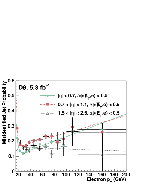
VII.1 Parameterization of the Misidentified Jet Probability

The measured probability for MJ events to enter the final electron plus two-jet selection sample is shown as a function of electron in Fig. 1. The MJ contribution in the electron channel arises from jets with a high enough fraction of energy deposited within the EM section of the calorimeter that they satisfy the electron identification criteria. Additional MJ backgrounds in the electron channel originate from the semileptonic decays of hadrons and from photons that are misidentified as electrons. The probability is measured separately in two CC regions ( and ) and separately in the EC region (). In each range of , the misidentified jet probability is parameterized as a function of electron in four intervals of the azimuthal separation of the electron and the vector (the four regions are shown combined for each interval in Fig. 1). In the CC region, the probabilities are parameterized as sums of exponentials and first-order polynomials in electron , whereas only a first-order polynomial in electron is used in the smaller statistics EC region. For the smaller statistics electron +3 jet sample, the probabilities are determined once for each region, and are applied to each interval separately after scaling to the average contribution obtained in that interval.
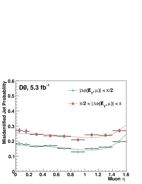
The measured probability for MJ background events to enter the final jet sample is shown as a function of muon in Fig. 2. The primary source of MJ background in the muon channel is from semileptonic decays of heavy quarks in which the decay muon satisfies the muon isolation criteria. The contribution of MJ events entering the loose sample is smaller in the muon channel than in the electron channel. Consequently, the misidentified jet probability is parameterized in only two regions [ and ] of azimuthal separation between the muon and the vectors. In both pre-2006 and post-2006 upgrade data, the misidentification probability is parameterized using a third-order polynomial in muon . The same functions are applied to both the muon +2 jet and +3 jet selected samples.
VIII Event Selection
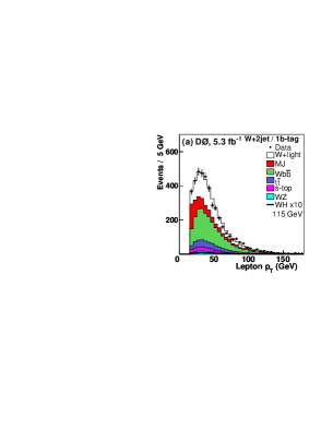
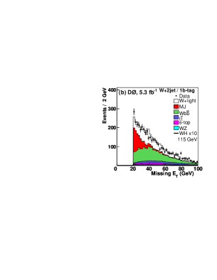
This section describes the selection of data samples containing events with a single reconstructed lepton, , and either two or three jets of transverse momentum , at least one of which is required to be consistent with having evolved from a quark. The samples are from data collected between 2002 and June 2009 at . Candidate bosons are selected by requiring an electron or a muon with transverse momenta and . Electrons are required to be in the pseudorapidity region or and muons in the region . The selected and candidate events are divided into samples containing exactly two or exactly three reconstructed jets. Jets are required to be in the region . A selection on the of the jets, and , is also applied to the +2 jet and +3 jet samples, respectively, and the event PV is required to be reconstructed within of the center of the detector. At least three charged tracks are required to be associated with that vertex.
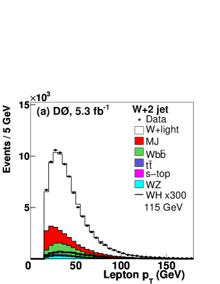
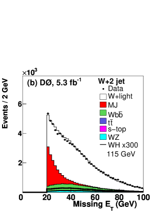
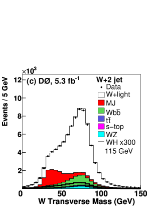
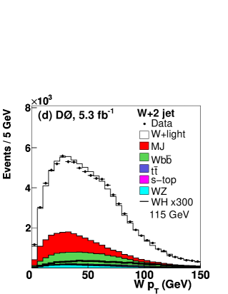
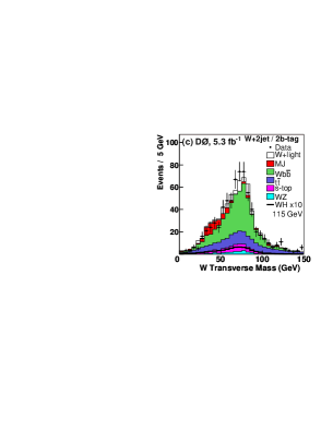
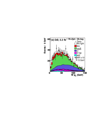
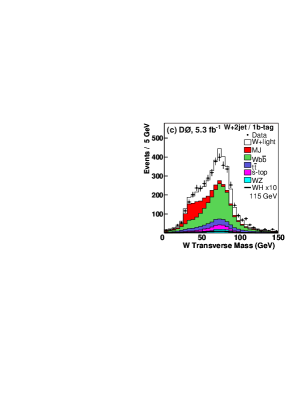
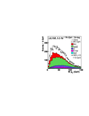
Distributions of lepton and are compared to the sum of the expected SM background contributions and data-determined MJ background for the +2 jet selected sample, which has the largest statistics of all selected samples, in Figs. 3(a) and (b). The electron and muon decay channel samples are combined in the figures, and all corrections to the background simulations have been applied. Details of the background estimates are given in Secs. VI and VII.
To suppress and background events and to avoid double counting events in Higgs searches based on dilepton final states, events with additional electrons or muons isolated from jets that pass and are rejected. Events containing isolated high- leptons that decay hadronically are also rejected by requiring or , depending on the decay channel tauid .
The transverse mass of the boson candidates () is reconstructed from the () system using the lepton transverse energy (), , and the azimuthal separation between the isolated lepton and the vector:
| (6) |
The distribution of for selected boson candidates is shown in Fig. 3(c). In addition to the dominant contribution from events with real boson decays, there is a significant component from MJ events that contributes mainly at small values of . Consequently the lower signal-to-background region at low is rejected by requiring
| (7) |
The distribution for the boson candidates is compared to the sum of the expected SM and MJ background contributions, prior to the requirement in Eq. 7, in Fig. 3(d).
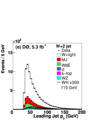
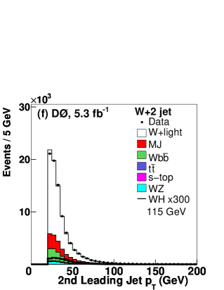
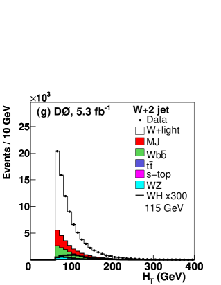
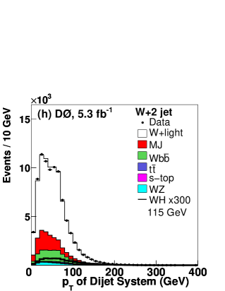
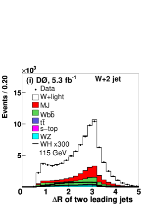
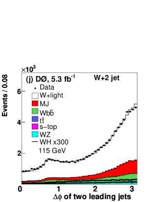
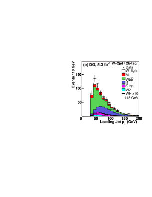
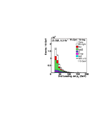
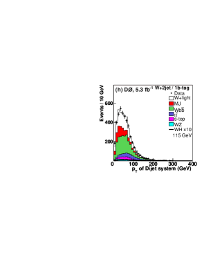
Kinematic jet properties for the selected +2 jet sample are also compared to the sum of the expected SM background contributions, including MJ background, in Fig. 3. The corrected electron and muon channel samples are combined in the figure. The background prediction provides an adequate description of the data for all the distributions.


To increase the final sensitivity, both the +2 jet and +3 jet samples are subdivided into statistically independent samples based on whether one or two of the leading jets in the event are consistent with having been initiated by a quark, as discussed in Sec. V. The first sample requires two jets, both with NN output values larger than a “loose” requirement (“loose-tag”). The second sample, selected from events that fail the two-tag requirement, requires a single jet with a NN output above a larger “tight” value requirement (“tight-tag”). In two--tagged jet events, the typical efficiency for identifying a jet that contains a hadron is % with a misidentification probability of 1.5% for light parton () initiated jets. In the single--tagged jet event sample, the typical efficiency for identifying a jet that contains a hadron is %, with a lower misidentification probability of 0.5% for light parton () initiated jets. The -tagging efficiency is treated separately from the jet taggability efficiency. Events that do not satisfy either of these tagging requirements are not considered further in the analysis.
The tagging efficiencies for jets that have passed the taggability requirements are studied in data and the efficiencies are applied to the simulation via event weights. These weights depend on the , , and partonic flavor of each tagged jet. In two -tagged events, the event weights are given by the product of the weights of the two -tagged jets. In single--tagged jet events, the final event weight also accounts for the simulated contribution of two--tagged jet events that “migrate” to the simulated single--tagged jet samples.
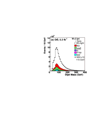
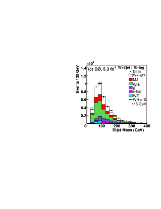
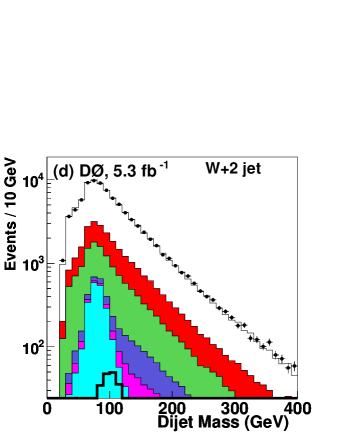
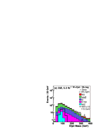
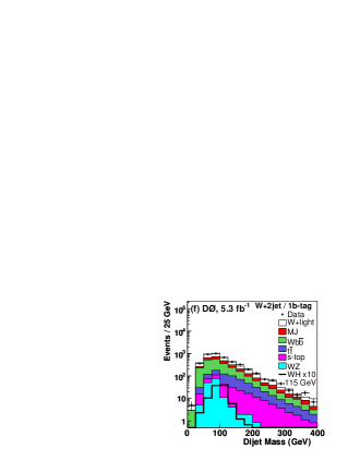
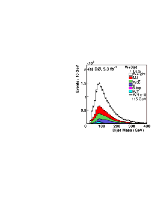
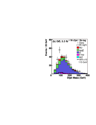
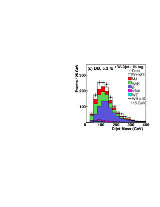
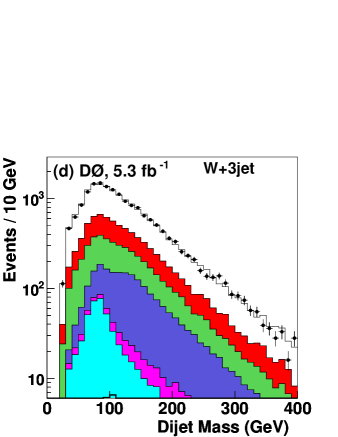
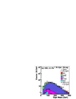
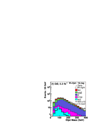
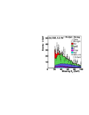
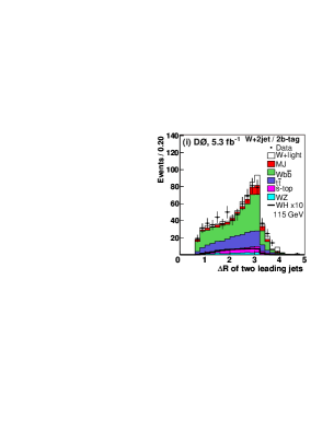
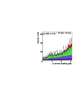
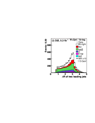
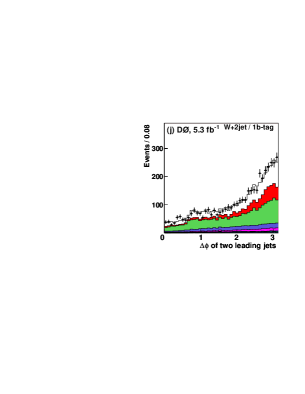
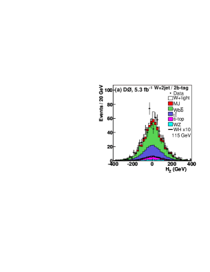
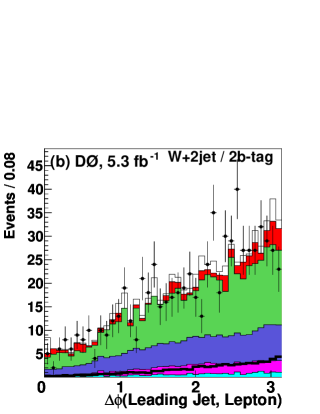
Distributions of dijet invariant mass, prior to -tagging, after requiring two -tags, and for single--tagged events, are shown for the +2 jet and +3 jet selections in Figs. 4 and 5, respectively. The sums of the expected backgrounds are compared to the data, and the electron and muon channel samples are again shown combined in each figure. Comparisons of kinematic properties in +2 jet events are shown in Figs. 6 and 7 for the two- and single--tagged samples, respectively. The expected signal contribution at is shown scaled by a factor of 10 in each figure.
The total event yields for each of the -tagged samples, in data and in simulation, are summarized in Table 2. In two--tagged jet events, the dominant backgrounds are from and processes. In single--tagged jet events, the dominant backgrounds are boson production in association with light or -quark jets as well as production and MJ events. The expected number of signal events in each sample is listed for an assumed Higgs mass . The uncertainties quoted are the combined statistical and systematic uncertainties, and the systematic uncertainties are those prior to the application of the fitting procedure applied when determining cross section upper limits described in Sec. XI.
| +2 jet | +2 jet | +3 jet | +3 jet | |||||||||
| 2 -tag | 1 -tag | 2 -tag | 1 -tag | |||||||||
| +light | 57.5 | 9.2 | 1290 | 201 | 12.1 | 1.8 | 210 | 35 | ||||
| MJ | 56.5 | 4.2 | 663 | 43 | 12.7 | 1.0 | 186 | 13 | ||||
| 346 | 93 | 1601 | 383 | 47.8 | 12.9 | 358 | 90 | |||||
| 177 | 35 | 417 | 54 | 176 | 35 | 633 | 96 | |||||
| s-top | 58.3 | 11.4 | 203 | 33 | 13.0 | 2.7 | 53.6 | 9.1 | ||||
| 22.5 | 3.3 | 152.6 | 17.6 | 2.6 | 1.1 | 33.9 | 4.8 | |||||
| Total | 718 | 120 | 4326 | 501 | 264 | 44 | 1474 | 160 | ||||
| Data | 709 | 4316 | 301 | 1463 | ||||||||
| 6.5 | 1.0 | 9.7 | 0.9 | 0.8 | 0.2 | 2.1 | 0.3 | |||||
IX Multivariate Discriminant
To separate the remaining background from the signal, a multivariate random forest (RF) discriminant technique RF1 ; RF2 is applied independently to each of the 16 subsamples, defined by categorizing events by lepton flavor (electron or muon), jet multiplicity (2 jets or 3 jets), -tag multiplicity (single- or two--tagged), and pre- and post-upgrade data. The RF technique employs a set of decision trees, each of which applies a series of consecutive binary decisions trained on simulated events of known origin until a predefined stopping configuration is reached. Half of the simulated events are used for training and validation, and the remaining half are used to estimate the relative contributions of signal and background in the data.
Each individual decision tree examines an initial input event training sample and applies selection criteria on a list of potentially discriminating variables to subdivide the training sample into smaller signal or background regions referred to as nodes. At each step, the selection criterion is chosen to maximize the positive cross entropy “figure of merit” value
| (8) |
where () is the fraction of correctly (incorrectly) classified events at each stage. The process is continued until a pure signal or pure background node is obtained, and the remaining node regions can no longer be further maximized and split without leaving fewer than a prespecified minimum number of events in the other daughter samples. The resulting output nodes are referred to as leaves.


| RF input variable | Description |
|---|---|
| Missing transverse energy | |
| Lepton- transverse mass | |
| (- system) | of boson candidate |
| () | Leading jet |
| () | Subleading jet |
| Dijet invariant mass | |
| (dijet system) | of dijet system |
| (,) | between the two leading jets |
| (,) | between the two leading jets |
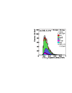
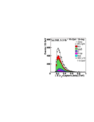
| Scalar sum of the transverse | |
| momenta of all jets in the event | |
| Scalar sum of the longitudinal | |
| momenta of all jets in the event | |
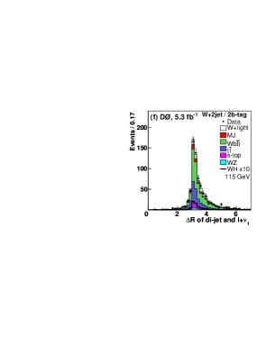
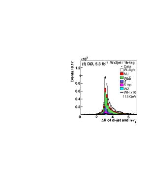
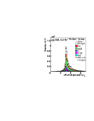
| (, ) | between the leading jet |
| and the lepton | |
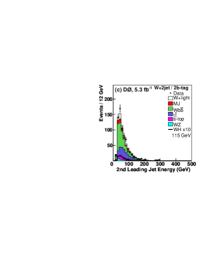
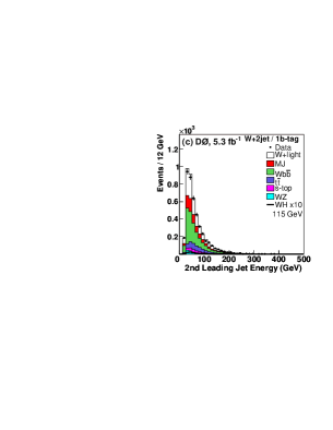
| Second leading jet energy | |
| Center-of-mass energy of the | |
| ++dijet system with larger | |
| solution for the longitudinal | |
| momentum of the candidate | |
| Center-of-mass energy of the | |
| ++dijet system with smaller | |
| solution for the longitudinal | |
| momentum of the candidate | |
| (dijet,) | between the dijet system |
| and the system with larger | |
| solution for the longitudinal | |
| momentum of the candidate | |
| (dijet,) | between the dijet system |
| and the system with smaller | |
| solution for the longitudinal | |
| momentum of the candidate | |
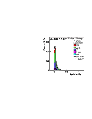
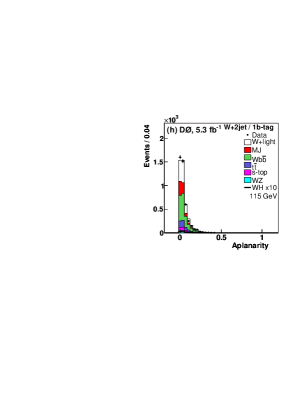
| Aplanarity | , where is the smallest |
| eigenvalue of the normalized | |
| momentum tensor: | |
| where runs over jets and | |
| the charged lepton and is | |
| the th 3-momentum component | |
| of the th physics object. | |
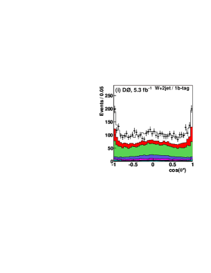
| Cosine of angle between the | |
| candidate and nominal proton | |
| beam direction in the zero | |
| momentum frame (see Ref. spincorr ) | |
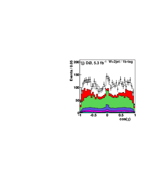
| Cosine of angle between lepton | |
| and rotated 3-momentum vector | |
| of the dijet system in the production | |
| plane of the boson rest frame spincorr |
For each of the subsamples, the decision tree algorithm is run multiple times to create the forest and variants of the default training sample are used for each decision tree within each RF. The outputs of the decision trees within each RF are combined to yield final RF output distributions. The decision tree samples are obtained using bootstrap aggregation (“bagging”), and a random subset of 13 of the 20 input discriminating variable distributions are assigned within each decision tree to create the forest. Varying the number of input variables used by is found to have a negligible effect on the RF output.
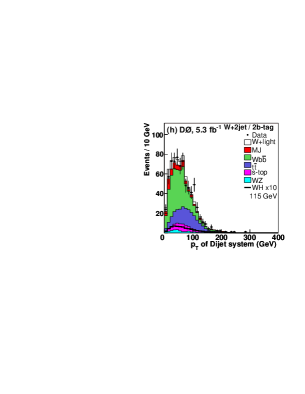
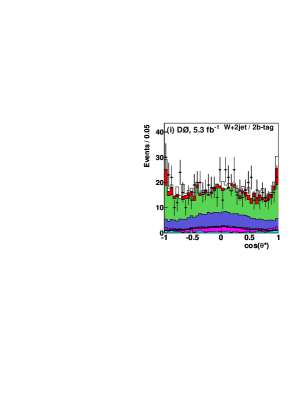
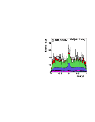
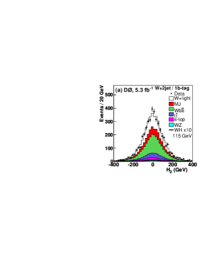
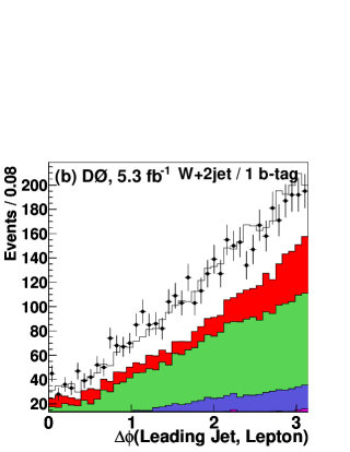
The 20 input variables used to build the RF decision are optimized in dedicated studies of their discriminating power and are listed, together with their definitions, in Table 3. Agreement between the data and the total MC and data-determined background estimates are obtained for each input variable distribution for both the two--tagged and single--tagged samples as well as for the full sample prior to the application of -tagging. The same set of input variables is used for the +2 jet and +3 jet samples. In addition to the ten variables already discussed in Sec. VIII, and displayed in Figs. 6 and 7, a further ten discriminating variables are provided to each RF and these are shown for the +2 jet sample, after the application of two and one -tag requirements to the events, in Figs. 8 and 9, respectively.
Two input distributions are provided for and (dijet,) corresponding to each of the two solutions for the longitudinal momentum component of the missing energy vector (assuming the lepton and are decay products of an on-shell boson). The angles and are included to exploit kinematic differences arising from the expected spin-0 nature of the Higgs and non-spin-0 nature of the background. The angle is the angle between the boson candidate and the nominal proton beam direction in the zero momentum frame, and is the angle between the charged decay lepton and rotated (production plane) three-momentum vector of the dijet system after boosting to the boson rest frame spincorr .
Each RF is trained simultaneously using all simulated backgrounds sources (the MJ contribution is excluded) for each simulated Higgs mass point, and the process is repeated for each of the 16 subsamples. The minimum number of events in a leaf is tuned in separate studies and the number that maximizes the sensitivity is selected. The number of decision trees used within each forest is also studied and tuned using the procedure of Ref. diboson .


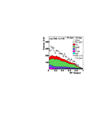
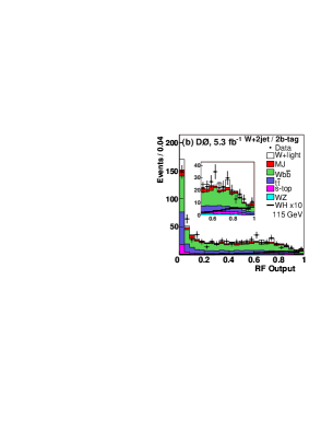
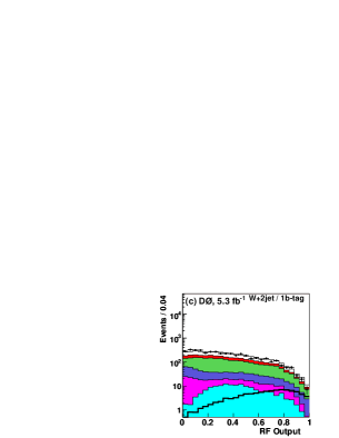
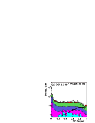
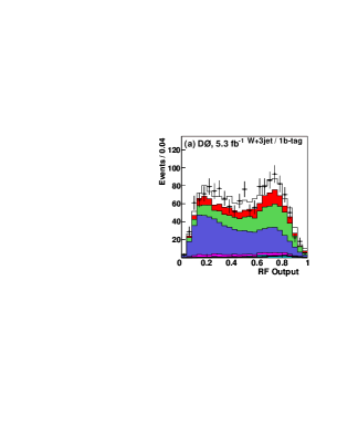
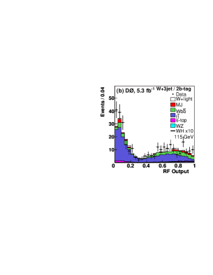
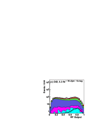
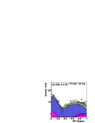
The resulting RF output distributions are shown in Figs. 10 and 11 for the two- and single--tagged jet requirements in the final +2 jet and +3 jet samples, respectively. The electron and muon channel samples have been combined in the figures, and the preupgrade and postupgrade samples are also combined in the figures. The figures show the results obtained using the signal samples. An improved separation of simulated signal and background contributions, is obtained in all cases.

X Systematic Uncertainties
The impact of each possible source of systematic uncertainty is assessed separately for the signal and for all backgrounds, for each of the 16 statistically independent samples, and categorized according to whether it affects the normalization and the shape (shape systematic) of the RF discriminant output distributions or whether it only affects the normalization of signal and backgrounds. A full analysis is repeated after individually varying each source by standard deviation (s.d.) in the simulation, except where noted otherwise (the uncertainty in the MJ background modeling is determined separately from data). After each variation, the simulated and MJ background yields are normalized to the selected data samples prior to the application of -tagging.
The systematic uncertainty assigned to the data-determined efficiency of the triggers used in the electron channel is (3–5)%. In the muon channel, where the full list of available triggers is used, a comparable uncertainty of (3–4)% is assigned. In the muon channel, this uncertainty arises from a normalization uncertainty of 2%, obtained after comparing results using the single high- muon and the full list of triggers, and a shape systematic of (1–3)% as a function of jet , applied to the non-single-muon trigger efficiency. The shape systematic is obtained by comparison of the single high- muon and non-single-muon triggered components of the dataset.
The uncertainty on the identification and reconstruction of isolated electrons, as well as their energies, affects the shapes of the electron channel RF distributions and is (5–6)%. In the muon channel, the uncertainty comprises three contributing sources: an uncertainty of 0.8% applied to the pre-upgrade muon identification efficiency (a 1.2% uncertainty is applied to the post-upgrade samples, which is increased for muon by adding 2% in quadrature), an uncertainty in the corresponding track reconstruction of 2.3% (pre-upgrade) and 1.4% (post-upgrade), and an uncertainty of 3.8% (pre-upgrade) and 0.9% (post-upgrade) on the scale factors used to correct the efficiencies for muons to pass isolation criteria in the MC to those measured in the data.
Sources of systematic uncertainty on the selection and reconstruction of jets are the jet resolution and jet energy scale, as well as the jet identification efficiency and vertex confirmation requirement (applied to the post-upgrade part of the dataset). Shape uncertainties for jet resolution and jet energy scale are determined by varying parameters in the jet resolution function and the energy scale correction and repeating the analysis using the kinematics of the modified jets. The size of this effect on the RF distribution depends on the sample and process and is in the range 15%-30%. The jet identification and vertex confirmation uncertainties are each determined by randomly reducing the number of jets that remain in simulation (the s.d. result is then obtained by inverting the s.d. result). The resulting RF shape systematic uncertainty is about 5%. Because of low statistics after -tagging for the +light and samples, the jet systematic uncertainties applied for these backgrounds are determined prior to -tagging.
The uncertainty on the jet taggability requirement is determined by varying the jet taggability correction factors. The taggability uncertainty affects the shapes of the RF output distributions and is about 3%. The RF shape uncertainty for the response of the -tagging algorithm is applied separately for light and heavy flavored jets and is typically (2.5–3.0)% for single-tagged heavy flavor jets and in the range (1–4)% for single-tagged light jets (the light-quark jet mistag probability uncertainty is of order 10%). The RF uncertainty is approximately doubled in the samples requiring two -tagged jets.
Uncertainties in the predicted , single top quark, and diboson cross sections are taken from ttbar_xsecs ; stop_xsecs ; mcfm and affect the normalizations of the backgrounds. The uncertainty on the CTEQ6L parton density function is estimated following the prescription of Ref. CTEQ . The alpgen-generated samples include additional normalization factors that change their visible cross sections, and their uncertainties are determined separately. The uncertainty in the reweighting procedure applied to the alpgen-generated event samples affects the shape of the alpgen RF output distributions and are typically of the order 2%. The uncertainty on the alpgen scale factor is 6% and the uncertainty on is 20%. The renormalization and factorization scales used in alpgen are varied by adjusting each scale simultaneously, by factors of 0.5 and 2.0. This affects the shapes of the alpgen RF output distributions, and the resulting uncertainty is of the order 2%, as is the uncertainty arising from the choice of value for the strong coupling constant . The uncertainty on the MLM factorization scheme used to match alpgen partons to cone jets is propagated to the RF distribution and results in a systematic uncertainty of about 2%.
The uncertainty in the MJ background modeling is obtained from the data. It is determined by varying the parameterization of the efficiency for loosely selected leptons to enter the final selected sample and by also varying the misidentified jet probabilities. The MJ uncertainties are anticorrelated with the normalization of the alpgen samples, and this is taken into account in the limit setting procedure. The overall experimental systematic uncertainty assigned to the distributions is about 6%. The uncertainty of the experimentally measured integrated luminosity is treated separately. The uncertainty is % lumi_ID and is fully correlated between all of the simulated background samples.
XI Upper Limits on the Cross Section
No excess of events is observed with respect to the background estimation and upper limits are therefore derived for the production cross section multiplied by the corresponding branching ratio in units of the SM prediction. The limits are calculated using the modified frequentist approach modfreq ; modfreq1 , and the procedure is repeated for each assumed value of .
Two hypotheses are considered: the background-only hypothesis (B), in which only background contributions are present, and the signal-plus-background (S+B) hypothesis in which both signal and background contributions are present.
The limits are determined using the RF output distributions, together with their associated uncertainties, as inputs to the limit setting procedure. To preserve the stability of the limit derivation procedure in regions of small background, the width of the bin at the largest RF output value is adjusted by comparing the total B and S+B expectations until the statistical significance for B and S+B is, respectively, greater than 3.6 and 5.0 standard deviations from zero. The remaining part of the distribution is then divided into 23 equally-sized bins. The rebinning procedure is checked for potential biases in the determination of the final limits, and no such bias is found.

The result for each hypothesis is obtained by testing the outcome of a large number of simulated pseudoexperiments. For each pseudoexperiment, pseudodata are drawn from the RF distributions, by randomly generating the pseudodata according to a Poisson statistical parent distribution for which the mean is either taken from the background-only or signal-plus-background hypothesis. A negative Poisson log likelihood ratio (LLR) test statistic is used to evaluate the statistical significance of each experiment, with the outcomes ordered in terms of their statistical significance. The frequency of each outcome defines the shapes of the resulting LLR distribution, for both the background-only and signal-plus-background hypotheses, at each mass point.
Systematic uncertainties are defined through nuisance parameters that are assigned Gaussian probability distributions (priors). The signal and background predictions are taken to be functions of the nuisance parameters and each nuisance parameter is sampled from a Gaussian probability distribution in each pseudoexperiment. The correlated systematic uncertainties across channels (such as the uncertainties on predicted SM cross sections, identification efficiencies, and energy calibration, as described in Sec. X) are also taken into account in the limit setting procedure collie .
The inclusion of systematic uncertainties in the generation of pseudoexperiments has the effect of broadening the LLR distributions and, thus, reducing the ability to resolve signal-like excesses. This degradation can be partially reduced by performing a maximum likelihood fit to each pseudoexperiment (and data), once each for the S+B and the background-only hypotheses. The maximization is performed over the systematic uncertainties. The LLR is evaluated for each outcome using the ratio of maximum likelihoods for the fit to each hypothesis. The resulting degradation of the limits due to systematic uncertainties is of the order of 30%.
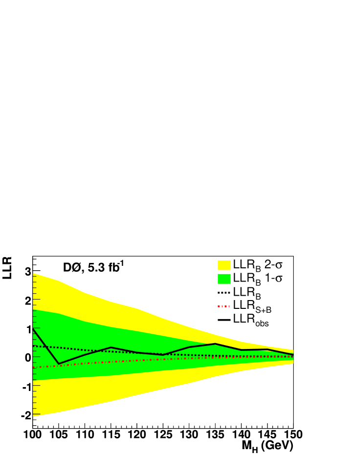
The medians of the obtained background-only LLR distributions for each tested mass point are summarized in Fig. 12. The resulting medians of the signal-plus-background hypothesis LLR distributions are also shown. The corresponding and values for the background-only hypothesis at each mass point are represented by the shaded regions in the figure. The LLR values obtained from the data are also summarized in the figure.
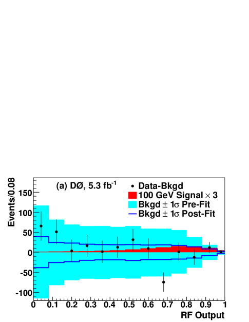
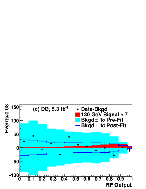
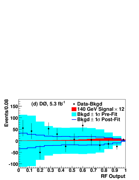
The RF discriminant distributions after the background-only profile fit are shown in Fig. 13 after subtracting the total background expectation, for the Higgs boson mass points and . The signal expectations are shown scaled to the final observed upper limits (rounded to the nearest integer) in each case, and the uncertainties in the background before and after the constrained fit are shown by the shaded bands and solid lines, respectively.
| Combined 95% C.L. Limit | ||
| Higgs Mass [GeV] | Expected | Observed |
| 100 | 3.3 | 2.7 |
| 105 | 3.6 | 4.0 |
| 110 | 4.2 | 4.3 |
| 115 | 4.8 | 4.5 |
| 120 | 5.6 | 5.8 |
| 125 | 6.8 | 6.6 |
| 130 | 8.5 | 7.0 |
| 135 | 11.5 | 7.6 |
| 140 | 16.5 | 12.2 |
| 145 | 23.6 | 15.0 |
| 150 | 36.8 | 30.4 |
Upper limits are calculated at 11 discrete values of the Higgs boson mass, spanning the range 100–150 GeV and spaced in units of 5 GeV, by scaling the expected signal contribution to the value at which it can be excluded at the 95% C.L. The expected limits are calculated from the background-only LLR distribution whereas the observed limits are quoted with respect to the LLR values measured in data. The expected and observed 95% C.L. upper limits results for the cross section multiplied by the branching ratio are shown, as a function of the Higgs boson mass , in units of the SM prediction in Fig. 14. The values obtained for the expected and observed limit to SM ratios at each mass point are listed in Table 4 (the uncertainty in the predicted cross section is available in Ref. signal ).
XII Summary
A search for the SM associated production in data corresponding
to an integrated luminosity of collected
with the D0 detector at the Fermilab Tevatron Collider shows no
excess beyond the expected contributions from SM backgrounds.
Statistically independent data samples containing
and candidates with either two
or three reconstructed jets in the event and subdivided into two -tagged jets or a single -tagged jet are analyzed
using a multivariate technique to provide separation of signal and background.
Upper limits are calculated at the 95% C.L.
for the cross section multiplied by the branching ratio for the region .
The
observed (expected) upper limits at 95% C.L. are a factor 4.5 (4.8)
larger than the SM expectation for a Higgs mass .
These results, combined with those of Ref. Aaltonen:2011rt and with other searches
in this mass region at the Tevatron, provide crucial constraints on the
Higgs coupling to , complementary to the information obtained,
for other decay modes, by the LHC experiments.
XIII Acknowledgments
We thank the staffs at Fermilab and collaborating institutions, and acknowledge support from the DOE and NSF (USA); CEA and CNRS/IN2P3 (France); MON, Rosatom and RFBR (Russia); CNPq, FAPERJ, FAPESP and FUNDUNESP (Brazil); DAE and DST (India); Colciencias (Colombia); CONACyT (Mexico); NRF (Korea); FOM (The Netherlands); STFC and the Royal Society (United Kingdom); MSMT and GACR (Czech Republic); BMBF and DFG (Germany); SFI (Ireland); The Swedish Research Council (Sweden); and CAS and CNSF (China).
References
- (1) The TEVNPH Working Group, arXiv:1107.5518 (2011), http://tevnphwg.fnal.gov.
- (2) V. M. Abazov et al. [D0 Collaboration], Phys. Lett. B 663, 26 (2008).
- (3) V. M. Abazov et al. [D0 Collaboration], Phys. Lett. B 698, 6 (2011).
- (4) L. Breiman, Machine Learning 45, 5 (2001).
- (5) I. Narsky, arXiv:physics/0507143 (2005); I. Narsky, arXiv:physics/0507157 (2005).
- (6) ALEPH, DELPHI, L3, and OPAL Collaborations, The LEP Working Group for Higgs Boson Searches, Phys. Lett. B 565, 61 (2003).
- (7) LEP, Tevatron, and SLD Electroweak Working Groups, arXiv: 0911.2604, http://lepewwg.web.cern.ch/LEPEWWG/.
- (8) V. M. Abazov et al. [D0 Collaboration], Phys. Rev. Lett. 94, 091802 (2005).
- (9) V. M. Abazov et al. [D0 Collaboration], Phys. Lett. B 663, 26 (2008).
- (10) V. M. Abazov et al. [D0 Collaboration], Phys. Rev. Lett. 102, 051803 (2009).
- (11) D. Acosta et al. [CDF Collaboration], Phys. Rev. Lett. 95, 051801 (2005).
- (12) T. Aaltonen et al. [CDF Collaboration], Phys. Rev. Lett. 100, 041801 (2008).
- (13) T. Aaltonen et al. [CDF Collaboration], Phys. Rev. Lett. 103, 101802 (2009).
- (14) T. Aaltonen et al. [CDF and D0 Collaborations], Phys. Rev. Lett. 104, 061802 (2010).
- (15) G. Aad et. al. [ATLAS Collaboration], arXiv:hep-ex/1202.1408 (2012), submitted to Phys. Lett. B, and references therein.
- (16) S. Chatrchyan et. al. [CMS Collaboration], arXiv:hep-ex/1202.1488 (2012), submitted to Phys. Lett. B, and references therein.
- (17) V. M. Abazov et al. [D0 Collaboration], Nucl. Instrum. Methods in Phys. Res. A 565, 463 (2006).
- (18) S. Abachi et al. [D0 Collaboration], Nucl. Instrum. Methods in Phys. Res. A 338, 185 (1994).
- (19) R. Angstadt et al., Nucl. Instrum. Methods in Phys. Res. A 622, 298 (2010).
- (20) V. M. Abazov et al. [D0 Collaboration], Nucl. Instrum. Methods in Phys. Res. A 552, 372 (2005).
- (21) S. Klimenko, J. Konigsberg, T. M. Liss, Fermilab-FN- 0741 (2003).
- (22) T. Andeen, et al., FERMILAB-TM-2365 (2007).
- (23) G. Boole, An Investigation of the Laws of Thought (Walton and Maberly, London, 1854) [www.gutenberg.org/ebooks/15114].
- (24) M. Abolins et al., Nucl. Instrum. Methods in Phys. Res. A 584, 75 (2008).
- (25) V. M. Abazov et al. [D0 Collaboration], Phys. Rev. D 76, 092007 (2007).
- (26) G. C. Blazey et al. arXiv:hep-ex/0005012 (2000).
- (27) V. M. Abazov et al. [D0 Collaboration], accepted by Phys. Rev. D. arXiv:hep-ex/1110.3771 (2011).
- (28) V. M. Abazov et al. [D0 Collaboration], Nucl. Instrum. Methods in Phys. Res. A 620, 490 (2010).
-
(29)
R. Brun and F. Carminati, CERN Program Library Long
Writeup, Report W5013 (1993);
M. Goossens et al., geant User’s Guide CERN, Geneva, 1994. - (30) M. Mangano et al., J. High Energy Phys. 07, 001 (2003). Version 2.05 was used.
- (31) R. Field, TeV4LHC Report of the QCD Working Group edited by M. G. Albrow et al., arXiv:hep-ph/0610012, 74 (2006). The results of Tune A were used.
- (32) T. Sjöstrand et al., pythia 6.3: Physics and Manual hep-ph/0308153 (2003).
- (33) K. A. Assamagan et al., arXiv:hep-ph/0406152.
- (34) O. Brein, A. Djouadi, and R. Harlander, Phys. Lett. B 579, 149 (2004).
- (35) M. L. Ciccolini, S. Dittmaier, and M. Kramer, Phys. Rev. D 68, 073003 (2003).
- (36) J. Baglio and A. Djouadi, J. High Energy Phys. 10, 064 (2010).
- (37) A. Djouadi, J. Kalinowski, and M. Spira, Comput. Phys. Commun. 108, 56 (1998).
- (38) T. Hahn et al., arXiv:hep-ph/0607308.
- (39) H. L. Lai et al., Phys. Rev. D 55 280 (1997); J. Pumplin et al., J. High Energy Phys. 07, 012 (2002).
- (40) J. Alwall et al., Eur. Phys. C 53, 473 (2008).
- (41) M. Mangano, M. Moretti and R. Pittau, Nucl. Phys. B 632 343 (2002).
- (42) N. Kidonakis et al., Phys. Rev. D 78, 074005 (2008).
- (43) A. Pukhov et al., hep-ph/9908288, (1999).
- (44) E. Boos et al., Nucl. Instrum. Methods in Phys. Res. A 534, 250 (2004).
- (45) N. Kidonakis, Phys. Rev. D 74, 114012 (2006).
- (46) J. M. Campbell and R. K. Ellis, Phys. Rev. D 60, 113006 (1999).
- (47) V. M. Abazov et al. [D0 Collaboration], Phys. Lett. B 669, 278 (2008).
- (48) V. M. Abazov et al. [D0 Collaboration], Phys. Lett. B 670, 292 (2009).
- (49) S. Parke and S. Veseli, Phys. Rev. D 60, 093003 (1999).
- (50) V. M. Abazov et al. [D0 Collaboration] Phys. Rev. Lett. 102, 161801 (2009).
- (51) T. Junk, Nucl. Instrum. Methods in Phys. Res. A 434, 435 (1999).
- (52) A. Read, J. Phys. G 28, 2693 (2002).
- (53) W. Fisher, FERMILAB-TM-2386-E (2007).
- (54) T. Aaltonen et al. [CDF Collaboration], Phys. Rev. D 85, 072001 (2012).