Restrictions and Extensions of Semibounded Operators

Abstract.

We study restriction and extension theory for semibounded Hermitian operators in the Hardy space $\mathscr{H}_{2}$ of analytic functions on the disk $\mathbb{D}$. Starting with the operator ${\displaystyle z\frac{d}{dz}}$, we show that, for every choice of a closed subset $F\subset\mathbb{T}=\partial\mathbb{D}$ of measure zero, there is a densely defined Hermitian restriction of ${\displaystyle z\frac{d}{dz}}$ corresponding to boundary functions vanishing on $F$. For every such restriction operator, we classify all its selfadjoint extension, and for each we present a complete spectral picture.

We prove that different sets $F$ with the same cardinality can lead to quite different boundary-value problems, inequivalent selfadjoint extension operators, and quite different spectral configurations. As a tool in our analysis, we prove that the von Neumann deficiency spaces, for a fixed set $F$, have a natural presentation as reproducing kernel Hilbert spaces, with a Hurwitz zeta-function, restricted to $F\times F$, as reproducing kernel.

To the memory of William B. Arveson.

1. Introduction

In this paper, we study a model for families of semibounded but unbounded selfadjoint operators in Hilbert space. It is of interest in our understanding of the spectral theory of selfadjoint operators arising from extension of a single semibounded Hermitian operator with dense domain. Up to unitary equivalence, the model represents a variety of spectral configurations of interest in the study of special functions, in the theory of Toeplitz operators, and in applications to quantum mechanics, and to signal processing.

We study a duality between restrictions and extensions of semibounded (unbounded) operators. Since the spectrum of a selfadjoint semibounded operator is contained in a half-line, it is useful to work with spaces of analytic functions. To narrow the field down to a manageable scope, we pick as Hilbert space the familiar Hardy space $\mathscr{H}_{2}$ of analytic functions on the complex disk $\mathbb{D}$ with square-summable coefficients. (As a Hilbert space, of course $\mathscr{H}_{2}$ is a copy of $l^{2}(\mathbb{N}_{0})$, but $l^{2}$ does not capture all the harmonic analysis of the Hardy space $\mathscr{H}_{2}$.)

Traditionally, the study of semibounded operators is viewed merely as a special case of the wider context of Hermitian, or selfadjoint operators. But semibounded does suggest that some measure (in this case, a spectral resolution) is supported in a halfline, say $[0,\infty)$, and thus, this in turn suggests analytic continuation, and Hilbert spaces of analytic functions (see, e.g., [ABK02]). In this paper, we take seriously this idea.

Now the operator ${\displaystyle H:=z\frac{d}{dz}}$ is selfadjoint on its natural domain in $\mathscr{H}_{2}$ with spectrum $\mathbb{N}_{0}$ (the natural numbers including $0$). We show (section 6) that, for every measure-zero closed subset $F$ of the circle $\mathbb{T}=\partial\mathbb{D}$, $H\>(={\displaystyle z\frac{d}{dz}})$ in $\mathscr{H}_{2}$ has a well defined and densely defined Hermitian restriction operator $L_{F}$, and we find its selfadjoint extensions. They are indexed by the unitary operators in a reproducing kernel Hilbert space (RKHS) of functions on $F$, where the reproducing kernel in turn is a restriction of Hurwitz’s zeta-function.

This RKHS-feature in the boundary analysis is one way that the boundary-value problems in Hilbert spaces of analytic functions are different from more traditional two sided boundary-value problems; see e.g., [JPT11a, JPT11b]. Two-sided boundary-value problems may be attacked with an integration by parts, or, in higher real dimensions, with Greens-Gauss-Stokes. By contrast, boundary-value theory is Hilbert spaces of analytic functions must be studied with the use of different tools.

While it is possible, for every subset $F$ of $\mathbb{T}$ (closed, measure zero), to write down parameters for all the selfadjoint extensions of $L_{F}$, to find more explicit formulas, and to compute spectra, it is helpful to first analyze the special case when the set $F$ is finite. Even the special case when $F$ is a singleton is of interest. We begin with a study of this in sections 3 and 4 below.

More generally, we show in section 6 that, when $F$ is finite, that then the corresponding Hermitian restriction operator $L_{F}$ has deficiency indices $(m,m)$ where $m$ is the cardinality of $F$. Moreover we prove that the variety of all selfadjoint extensions of $L_{F}$ will then be indexed (bijectively) by a compact Lie group $G(F)$ depending on $F$.

There is a number of differences between boundary value problems in $L^{2}$-spaces of functions in real domains, and in Hilbert spaces of analytic functions.

Our present study is confined here to one complex variable, and to the Hardy-space $\mathscr{H}_{2}$ on the disk $\mathbb{D}$ in the complex plane. The occurrence of the above mentioned family of compact Lie groups is one way our analysis of extensions and restrictions of operators is different in the complex domain.

There are others (see section 6 for details). Here we outline one such striking difference:

Recall that for a Hermitian partial differential operators $P$ acting on test functions in bounded open domains $\Omega\subset\mathbb{R}^{n}$, the adjoint operators will again act as PDOs.

Specifically, in studying boundary value problems in the Hilbert space $L^{2}(\Omega)$, initially one takes a given Hermitian $P$ to be defined on a Schwartz space of functions on $\Omega$, vanishing with all their derivatives on $\partial\Omega$. This realization of $P$ is called the minimal operator, $P_{min}$ for specificity, and it is $L^{2}$-Hermitian with dense domain in $L^{2}(\Omega)$.

The adjoint of $P_{min}$ is denoted $P^{*}$ and it is defined relative to the inner product in the Hilbert space $L^{2}(\Omega)$. And this adjoint is the maximal operator $P_{max}$. The crucial fact is that $P_{max}$ is again a (partial) differential operator. Indeed it is the operator $P$ acting on the domain of functions $f\in L^{2}(\Omega)$ such that $Pf$ is again in $L^{2}(\Omega)$, where the meaning of $Pf$ in the weak sense of distributions. This follows conventions of L. Schwartz, and K. O. Friedrichs; see e.g., [DS88b, Gru09, AB09].

Turning now to the complex case, we study here the operator ${\displaystyle Q:=z\frac{d}{dz}}$ in the Hardy-space $\mathscr{H}_{2}$ on the disk $\mathbb{D}$, and its realization as a Hermitian operator with domain equal to one in a family of suitable dense linear subspaces in $\mathscr{H}_{2}$. These Hermitian operators will have equal deficiency spaces (in the sense of von Neumann), and they will depend on conditions assigned on chosen closed subsets $F\subset\partial\mathbb{D}$), of (angular) measure 0.

When such a subset $F$ is given, let $Q_{F}$ be the corresponding restriction operator. But now the adjoint operators $Q_{F}^{*}$, defined relative to the inner product in $\mathscr{H}_{2}$, turn out no longer to be differential operators; they are different operators. The nature of these operators $Q_{F}^{*}$ is studied in sect 6.5.

In section 6, we study the operator ${\displaystyle z\frac{d}{dz}}$ in the Hardy space $\mathscr{H}_{2}$ of the disk $\mathbb{D}$, one such Hermitian operator $L_{F}$ for each closed subset $F\subset\partial\mathbb{D}$ of zero angular measure. For functions $f\in\mathscr{D}(L_{F}^{*})$ we have boundary values $\tilde{f}$, i.e., extensions from $\mathbb{D}$ to $\overline{\mathbb{D}}$ (= closure). But then the function ${\displaystyle z\frac{d}{dz}f}$ may have simple poles at the points $\zeta\in F$. We show (Corollary 6.33) that the contribution to $\boldsymbol{B}_{F}(f,f)$ (see (1.6)) is

$$\boldsymbol{B}_{F}(f,f)_{\zeta}=\Im\left(C_{\zeta}(f)\overline{\tilde{f}(\zeta)}\right)$$ (1.1)

where $\Im$ stands for imaginary part, and $C_{\zeta}(f)$ is the residue of the meromorphic function ${\displaystyle z\mapsto z\left(\frac{d}{dz}f\right)\left(z\right)}$ at the pole $z=\zeta$ ($\in F\subset\partial\mathbb{D}$.)

Note that (1.1), for the boundary form in the study of deficiency indices in the Hardy space $\mathscr{H}_{2}$, contrasts sharply with the more familiar analogous formula for the boundary value problems in the real case, i.e., on an interval.

In section 8, we consider a higher dimensional version of the Hardy-Hilbert space $\mathscr{H}_{2}$, the Arveson-Drury space $\mathscr{H}_{d}^{(AD)}$, $d>1$. While the case $d>1$ does have a number of striking parallels with $d=1$, there are some key differences. The reason for the parallels is that the reproducing kernel, the Szegö kernel for $\mathscr{H}_{2}$ extends from one complex dimension to $d>1$ almost verbatim, [Arv98, Dru78].

A central theme in our paper ($d=1$) is showing that the study of von Neumann boundary theory for Hermitian operators translates into a geometric analysis on the boundary of the disk $\mathbb{D}$ in one complex dimension, so on the circle $\partial\mathbb{D}$.

We point out in sect 8 that multivariable operator theory is more subtle. Indeed, Arveson proved [Arv98, Coroll 2] that the Hilbert norm in $\mathscr{H}_{d}^{(AD)}$, $d>1$, cannot be represented by a Borel measure on $\mathbb{C}^{d}$. So, in higher dimension, the question of "geometric boundary" is much more subtle.

1.1. Unbounded Operators

Before passing to the main theorems in the paper, we recall a classification theorem of von Neumann which will be used. Starting with a fixed Hermitian operator with dense domain in Hilbert space, and equal indices, von Neumann’s classification ([vN32b, vN32a, AG93, DS88b, Kat95]) shows that the variety of all selfadjoint extensions, and their spectral theory, can be understood and classified in the language of an associated boundary form, and the set of all partial isometries between a pair of deficiency-spaces. It has numerous applications. One significance of the result lies in the fact that the two deficiency-spaces typically have a small dimension, or allow for a reduction, reflect an underlying geometry, and they are computable.

Lemma 1.1 (see e.g. [DS88b]).

Let $L$ be a closed Hermitian operator with dense domain $\mathscr{D}_{0}$ in a Hilbert space. Set

$$\mathscr{D}_{\pm} =\{\psi_{\pm}\in dom(L^{*})\left.\right|L^{*}\psi_{\pm}=\pm i\psi_{\pm}\}$$

$$\mathscr{C}(L) =\{U:\mathscr{D}_{+}\rightarrow\mathscr{D}_{-}\left.\right|U^{*}U=P_{\mathscr{D}_{+}},UU^{*}=P_{\mathscr{D}_{-}}\}$$ (1.2)

where $P_{\mathscr{D}_{\pm}}$ denote the respective projections. Set

$$\mathscr{E}(L)=\{S\left.\right|L\subseteq S,S^{*}=S\}.$$

Then there is a bijective correspondence between $\mathscr{C}(L)$ and $\mathscr{E}(L)$, given as follows:

If $U\in\mathscr{C}(L)$, and let $L_{U}$ be the restriction of $L^{*}$ to

$$\{\varphi_{0}+f_{+}+Uf_{+}\left.\right|\varphi_{0}\in\mathscr{D}_{0},f_{+}\in\mathscr{D}_{+}\}.$$ (1.3)

Then $L_{U}\in\mathscr{E}(L)$, and conversely every $S\in\mathscr{E}(L)$ has the form $L_{U}$ for some $U\in\mathscr{C}(L)$. With $S\in\mathscr{E}(L)$, take

$$U:=(S-iI)(S+iI)^{-1}\left.\right|_{\mathscr{D}_{+}}$$ (1.4)

and note that

1. $U\in\mathscr{C}(L)$, and

2. $S=L_{U}$.

Vectors $f\in dom(L^{*})$ admit a unique decomposition

$$f=\varphi_{0}+f_{+}+f_{-}$$ (1.5)

where $\varphi_{0}\in dom(L)$, and $f_{\pm}\in\mathscr{D}_{\pm}$. For the boundary-form $\mathbf{B}(\cdot,\cdot)$, we have

$$\mathbf{B}(f,f) =\frac{1}{2i}\left(\left\langle L^{*}f,f\right\rangle-\left\langle f,L^{*}f\right\rangle\right)$$

$$=\left\|f_{+}\right\|^{2}-\left\|f_{-}\right\|^{2}.$$ (1.6)

Note, the sesquilinear form $\boldsymbol{B}$ in (1.6) is the boundary form referenced in (1.1) above.

Proof sketch (Lemma 1.1).

We refer to the cited references for details. The key step in the verification of formula (1.6) for the boundary form $\boldsymbol{B}(f,f)$, $f\in dom(L^{*})$, is as follows: Let $f=\varphi_{0}+f_{+}+f_{-}$. After each of the two terms $\left\langle L^{*}f,f\right\rangle$ and $\left\langle f,L^{*}f\right\rangle$ are computed, we find cancellation upon subtraction, and only the two $\left\|f_{\pm}\right\|^{2}$ terms survive; specifically:

$$\left\langle L^{*}f,f\right\rangle-\left\langle f,L^{*}f\right\rangle$$

$$= i\left(\left\|f_{+}\right\|^{2}-\left\|f_{-}\right\|^{2}\right)-(-i)\left(\left\|f_{+}\right\|^{2}-\left\|f_{-}\right\|^{2}\right)$$

$$= 2i\left(\left\|f_{+}\right\|^{2}-\left\|f_{-}\right\|^{2}\right).$$

∎

While there are earlier studies of boundary forms (in the sense of (1.6)) in the context of Sturm-Liouville operators, and Hermitian PDOs in bounded domains in $\mathbb{R}^{n}$, e.g., [BMT11, BL10], there appear not to be prior analogues of this in Hilbert spaces of analytic functions in bounded complex domains.

Terminology. We shall refer to eq. (1.5) as the von Neumann decomposition; and to the classification of the family of all selfadjoint extensions (see (1.3) & (1.4)) as the von Neumann classification.

Lemma 1.2.

1. Consider the von Neumann decomposition

   $$\mathscr{D}(L^{*})=\mathscr{D}(L)+\mathscr{D}_{+}+\mathscr{D}_{-}$$ (1.7)

   in (1.5); then the boundary form $\boldsymbol{B}(f,g)$ vanishes if one of the vectors $f$ or $g$ from $\mathscr{D}(L^{*})$ is in $\mathscr{D}(L)$.

2. Every subspace $S\subset\mathscr{D}(L^{*})$ such that $\boldsymbol{B}(f,f)=0$, $\forall f\in S$, is the graph of a partial isometry from $\mathscr{D}_{+}$ into $\mathscr{D}_{-}$.

3. Introducing the inner product

   $$\left\langle f,g\right\rangle_{*}=\left\langle f,g\right\rangle+\left\langle L^{*}f,L^{*}g\right\rangle$$ (1.8)

   $f,g\in\mathscr{D}(L^{*})$, we note that the three terms in the decomposition (1.7) are mutually orthogonal w.r.t. the inner product $\left\langle\cdot,\cdot\right\rangle_{*}$ in (1.8).

Proof.

All assertions (1)-(3) follow from a direct computation, and use of the definitions.

It follows from (2) in Lemma 1.2, that the boundary form $\boldsymbol{B}(\cdot,\cdot)$ passes to the quotient $\left(\mathscr{D}(L^{*})/\mathscr{D}(L)\right)\times\left(\mathscr{D}(L^{*})/\mathscr{D}(L)\right)$. ∎

1.2. Graphs of Partial Isometries $\mathscr{D}_{+}\longrightarrow\mathscr{D}_{-}$

In section 6, we will compute the partial isometries between defect spaces in a Hardy space $\mathscr{H}_{2}$ in terms of boundary values and residues. But we begin with axioms of the underlying geometry in Hilbert space.

Lemma 1.3.

Let $L$ be a Hermitian symmetric operator with dense domain in a Hilbert space $\mathscr{H}$, and let $x_{\pm}\in\mathscr{D}_{\pm}$ be a pair of vectors in the respective deficiency-spaces. Suppose

$$\left\|x_{+}\right\|=\left\|x_{-}\right\|>0.$$ (1.9)

Then the system

$$\begin{cases}{\displaystyle y_{2}:=\frac{1}{2i}\left(x_{+}-x_{-}\right)}\\ \\ {\displaystyle y_{3}:=\frac{1}{2}\left(x_{+}+x_{-}\right)}\end{cases}$$ (1.10)

satisfy $y_{i}\in\mathscr{D}(L^{*})$, $i=2,3,$ and

$$L^{*}y_{2}=y_{3},\mbox{ and }L^{*}y_{3}=-y_{2}.$$ (1.11)

Conversely, if $\left\{y_{2},y_{3}\right\}$ is a pair of non-zero vectors in $\mathscr{D}(L^{*})$ such that (1.11) holds; then

$$\begin{cases}x_{+}=y_{3}+iy_{2}\in\mathscr{D}_{+}&\mbox{and}\\ x_{-}=y_{3}-iy_{2}\in\mathscr{D}_{-},\end{cases}$$ (1.12)

and (1.9) holds.

Proof.

The result follows from Lemmas 1.1 and 1.2 together with a simple computation.∎

Corollary 1.4.

Let $L$ and $\mathscr{D}_{\pm}$ (deficiency-spaces) be as in the lemma. Let $U:\mathscr{D}_{+}\longrightarrow\mathscr{D}_{-}$ be a partial isometry, and let $x_{+}$ be in the initial space of $U$. Then the Hermitian extension $H$ of $L$ given by

$$H\left(x_{+}+Ux_{+}\right)=i\left(x_{+}-Ux_{+}\right)$$ (1.13)

is specified equivalently by the two vectors $y_{2}$ and $y_{3}$ as follows:

$$y_{2}\in\mathscr{D}(H)\;\mbox{and}\ Hy_{2}=y_{3};\;\mbox{or }y_{3}\in\mathscr{D}(H)\>\mbox{and }Hy_{3}=-y_{2}$$ (1.14)

where

$$\begin{cases}y_{2}={\displaystyle\frac{1}{2i}\left(x_{+}-Ux_{+}\right)},&\mbox{and}\\ \\ y_{3}={\displaystyle\frac{1}{2}\left(x_{+}+Ux_{+}\right)}.\end{cases}$$ (1.15)

In particular, for the boundary form $\boldsymbol{B}(\cdot,\cdot)$ on $\mathscr{D}(L^{*})$ from (1.6), we have $\boldsymbol{B}(y_{i},y_{i})=0$ for $i=2,3$.

Proof.

This follows from the lemma since a pair of vectors $x_{\pm}\in\mathscr{D}_{\pm}$ is in the graph of a partial isometry $\mathscr{D}_{+}\longrightarrow\mathscr{D}_{-}$ if and only if (1.9) holds. ∎

1.3. Prior Literature

There are related investigations in the literature on spectrum and deficiency indices. For the case of indices $(1,1)$, see for example [ST10, Mar11]. For a study of odd-order operators, see [BH08]. Operators of even order in a single interval are studied in [Oro05]. The paper [BV05] studies matching interface conditions in connection with deficiency indices $(m,m)$. Dirac operators are studied in [Sak97]. For the theory of selfadjoint extensions operators, and their spectra, see [Šmu74, Gil72], for the theory; and [Naz08, VGT08, Vas07, Sad06, Mik04, Min04] for recent papers with applications. For applications to other problems in physics, see e.g., [AHM11, PR76, Bar49, MK08]. And [Chu11] on the double-slit experiment. For related problems regarding spectral resolutions, but for fractal measures, see e.g., [DJ07, DHJ09, DJ11].

The study of deficiency indices $(n,n)$ has a number of additional ramifications in analysis: Included in this framework is Krein’s analysis of Voltera operators and strings; and the determination of the spectrum of inhomogenous strings; see e.g., [DS01, KN89, Kre70, Kre55].

Also included is their use in the study of de Branges spaces, see e.g., [Mar11], where it is shown that any regular simple symmetric operator with deficiency indices $(1,1)$ is unitarily equivalent to the operator of multiplication in a reproducing kernel Hilbert space of functions on the real line with a sampling property). Further applications include signal processing, and de Branges-Rovnyak spaces: Characteristic functions of Hermitian symmetric operators apply to the cases unitarily equivalent to multiplication by the independent variable in a de Branges space of entire functions.

1.4. Organization of the Paper

The central themes in our paper are presented, in their most general form, in sections 6 and 7. However, in sections 2 through 5, we are preparing the ground leading up to section 6, beginning with some lemmas on unbounded operators in section 2.

Further in sections 3 and 4 (before introducing harmonic analysis in the Hardy space $\mathscr{H}_{2}$), we begin with an analysis of model operators in the Hilbert space $l^{2}(\mathbb{N}_{0})$. In sections 3 and 4, it will be helpful to restrict our analysis to the case of deficiency indices $(1,1)$.

The reason for beginning with the Hilbert space $l^{2}(\mathbb{N}_{0})$ is that some computations are presented more clearly there. But they will then be used in section 6 where we introduce operators in the Hardy space $\mathscr{H}_{2}$ (of analytic functions on the disk $\mathbb{D}$ with $l^{2}$-coefficients.)

It is only with the use of kernel theory for $\mathscr{H}_{2}$, and its subspaces, that we are able to make precise our results for the case of deficiency indices $(m,m)$ where $m$ can be any number in $\mathbb{N}\cup\{\infty\}$. For the case when our operators have indices $(m,m)$, $m>1$, the possibilities encompass a rich variety. Indeed, there is a boundary value problem for every choice of a closed subset $F\subset\mathbb{T}=\partial\mathbb{D}$ of measure zero. In fact we prove that even different sets $F$ with the same cardinality can lead to quite different boundary-value problems, inequivalent extension operators, and quite different spectral configurations for the selfadjoint extensions.

2. Restrictions of Selfadjoint Operators

The general setting here is as sketched above; see especially Lemma 1.1, a statement of von Neumann’s theorem yielding a classification of the selfadjoint extensions of a fixed Hermitian operator $L$ with dense domain in a given Hilbert space $\mathscr{H}$, and $L$ having equal deficiency indices.

Below we will be concerned with the converse question: Given an unbounded selfadjoint operator in $\mathscr{H}$; what are the parameters for the variety of all closed Hermitian restrictions having dense domain in $\mathscr{H}$. The answer is given below, where we further introduce the restriction on the possibilities by the added requirement of semi-boundedness.

Our main reference regarding unbounded operators in Hilbert space will be [DS88b], but we will be relying too on results from [AG93] on spectral theory in the case of indices $(m,m)$ with $m$ finite, [Kat95] on closed quadratic forms, and [Gru09] for distribution theory and semibounded operators.

2.1. Conventions and Notation.

• $\mathscr{H}$ - a complex Hilbert space;

• $H$ - selfadjoint operator in $\mathscr{H}$;

• $\mathscr{D}(H)$ - domain of $H$, dense in $\mathscr{H}$;

• For $\xi\in\mathbb{C}$, $\Im(\xi)\neq 0$, the resolvent operator

  $$R(\xi)=(\xi I-H)^{-1}$$

  is well defined; it is bounded, i.e.,

  $$\left\|R(\xi)\right\|_{\mathscr{H}\rightarrow\mathscr{H}}\leq\left|\Im(\xi)\right|^{-1},\;\mbox{and}$$ (2.1)

  $$R(\xi)^{*}=R(\overline{\xi})$$ (2.2)

• $\perp$ - orthogonal complement.

Question: What are the closed restriction operators $L$ for $H$, such that $\mathscr{D}(L)$ is dense, where $\mathscr{D}(L)$ is the domain of $L$?

The answer is given in the following lemma:

Lemma 2.1.

Let $\mathscr{H}$, $H$, and $\xi$, be as above, in particular, $\Im(\xi)\neq 0$ is fixed. Then there is a bijective correspondence between (1) and (2) as follows:

1. $L$ is a closed restriction of $H$ with dense domain $\mathscr{D}(L)$ in $\mathscr{H}$; and

2. $\mathfrak{M}$ is a closed subspace in $\mathscr{H}$ such that

   $$\mathfrak{M}\cap\mathscr{D}(H)=0;$$ (2.3)

   where the correspondence $L$ to $\mathfrak{M}$ is

   $$\mathfrak{M}=\{\psi\in\mathscr{H}\>\big{|}\>\psi\in\mathscr{D}(L^{*}),L^{*}\psi=\xi\psi\};$$ (2.4)

   while, from $\mathfrak{M}$ to $L$, it is:

   $$\mathscr{D}(L)=\left(R(\overline{\xi})\>\mathfrak{M}\right)^{\perp}.$$ (2.5)

Proof.

From (1) to (2). Let $L$ be a restriction operator as in (1), i.e., with $\mathscr{D}(L)$ dense in $\mathscr{H}$. Then $L$ is Hermitian, and therefore,

$$L\subset L^{*}.$$ (2.6)

It follows in particular that $\mathscr{D}(L^{*})$ is also dense.

By von Neumann’s theory, [DS88b], we conclude that, for every $\xi\in\mathbb{C}$ s.t. $\Im(\xi)\neq 0$, the subspaces $\mathfrak{M}_{\xi}$ in (2.4) have the same dimension. In particular, $L$ has deficiency indices $(n,n)$ where $n=\mbox{dim }\mathfrak{M}$. We pick a fixed $\xi\in\mathbb{C}$, $\Im(\xi)\neq 0$. It further follows from [DS88a] that $\mathfrak{M}$ is closed.

We now prove that $\mathfrak{M}$ satisfies (2.3). If $\mathfrak{M}=0$, there is nothing to prove. Now suppose $\psi\in\mathfrak{M}$ and $\psi\neq 0$. Since $L\subseteq H$, from (2.6) we get

$$L\subset H\subset L^{*},$$ (2.7)

and therefore if $\psi\in\mathscr{D}(H)$, it follows that

$$\left\langle\psi,L^{*}\psi\right\rangle=\left\langle\psi,H\psi\right\rangle\in\mathbb{R}.$$

But (2.4) implies:

$$\left\langle\psi,L^{*}\psi\right\rangle=\xi\left\langle\psi,\psi\right\rangle=\xi\left\|\psi\right\|^{2}.$$ (2.8)

Since $\Im(\xi)\neq 0$, we have a contradiction. Hence (2.3) must hold.

From (2) to (1). Let $\mathfrak{M}$ be a closed subspace satisfying (2.3). Then define the subspace $\mathscr{D}(L)$ as in (2.5). Let $L:=H\big{|}_{\mathscr{D}(L)}$, i.e., defined to be the restriction of $H$ to this subspace.

The key step in the argument is the assertion that $\mathscr{D}(L)$, so defined, is dense in $\mathscr{H}$. We will prove the implication:

$$\psi\in\mathscr{D}(L)^{\perp}\Longrightarrow\psi=0$$ (2.9)

By (2.5), we have

$$\mathscr{D}(L)=\left(R(\overline{\xi})\>\mathfrak{M}\right)^{\perp}=R(\xi)\left(\mathfrak{M}^{\perp}\right).$$

Hence, $\psi\in\mathscr{D}(L)^{\perp}$ $\Longleftrightarrow$

$$\left\langle R(\overline{\xi})\psi,m^{\perp}\right\rangle=\left\langle\psi,\underset{\in\mathscr{D}(L)}{\underbrace{R(\xi)m^{\perp}}}\right\rangle=0,\>\forall m^{\perp}\in\mathfrak{M}^{\perp}.$$

But $\mathfrak{M}=\mathfrak{M}^{\perp\perp}$, since $\mathfrak{M}$ is closed. Hence $R(\overline{\xi})\psi\in\mathfrak{M}\cap\mathscr{D}(H)=0$; and therefore $\psi=0$; which proves (2.9). ∎

2.2. The Case When $H$ is Semibounded

There is an extensive general theory of semibounded Hermitian operators with dense domain in Hilbert space, [AG93, DS88b, Kat95]. One starts with a fixed semibounded Hermitian operator $L$, and then passes to a corresponding quadratic form $q_{L}$ [Kat95]. The lower bound for $L$ is defined from $q_{L}$.

Now, the initial operator $L$ will automatically have equal deficiency indices, and, in the general case (Lemma 2.1), there is therefore a rich variety of possibilities for the selfadjoint extensions of $L$ . In this paper, we will be concerned with particular model examples of semibounded operators, typically have much more restricted parameters for their selfadjoint extensions than what is possible for more general semibounded operators. Nonetheless, there are many instances of operators arising in applications which are unitarily equivalent to the “simple” model. Some will be discussed in detail in sections 5 and 6 below.

Definition 2.2.

We say that a Hermitian operator $L$ with dense domain $\mathscr{D}(L)$ in a fixed Hilbert space $\mathscr{H}$ is semibounded if there is a number $b>-\infty$ such that

$$\left\langle x,Lx\right\rangle\geq b\left\|x\right\|^{2},\>\mbox{for all }x\in\mathscr{D}(L).$$ (2.10)

Then the best constant $b$, valid for all $x$ in (2.10), will be called the greatest lower bound (GLB.)

Lemma 2.3.

Suppose a selfadjoint operator $H$ has a lower bound $b$. If $c\in\mathbb{R}$ satisfies $-\infty<c<b$, then, in the parameterization from Lemma 2.1, we may take

$$\mathfrak{M}=\{\psi\in\mathscr{H}\>\big{|}\>\psi\in\mathscr{D}(L^{*}),\>L^{*}\psi=c\,\psi\},$$ (2.11)

and, in the reverse direction,

$$\mathscr{D}(L)=\left((H-cI)^{-1}\mathfrak{M}\right)^{\perp}.$$ (2.12)

This will again be a bijective correspondence between:

1. all the closed and densely defined restrictions $L$ of $H$, and

2. all the closed subspaces $\mathfrak{M}$ in $\mathscr{H}$ satisfying

   $$\mathfrak{M}\cap\mathscr{D}(H)=\{0\}.$$ (2.13)

Proof.

The argument is the same as that used in the proof of Lemma 2.1, mutatis mutandis. ∎

3. Semibounded Operators

Below we consider the particular semibounded Hermitian operator $L$ with its dense domain in the Hilbert space $l^{2}(\mathbb{N}_{0})$ of square-summable one-sided sequences. (Our justification for beginning with $l^{2}$ is the natural and known isometric isomorphism $l^{2}\simeq\mathscr{H}_{2}$ (with the Hardy space); see [Rud87] and section 6 below for details.) It is specified by a single linear condition, see (3.3) below, and is obtained as a restriction of a selfadjoint operator $H$ in $l^{2}(\mathbb{N}_{0})$ having spectrum $\mathbb{N}_{0}$. While $0$ is in the bottom of the spectrum of $H$, it is not a priori clear that the greatest lower bound for its restriction $L$ will also be $0$, (see sect. 5 for details.) After all, finding the lower bound for $L$ is a quadratic optimization problem with constraints. Nonetheless we prove (Lemma 5.1) that $L$ also has $0$ as its lower bound.

For $p>0$, let $\ell^{p}$ be the set of complex sequence ${\displaystyle x=(x_{k})_{k=0}^{\infty}}$ such that ${\displaystyle\sum\left|x_{k}\right|^{p}}<\infty$. The operator ${\displaystyle H\left(x_{k}\right)=\left(kx_{k}\right)}$ with domain

$${\displaystyle\mathscr{D}(H)=\{x\in\ell^{2}:Hx\in\ell^{2}\}}$$ (3.1)

is selfadjoint in the Hilbert space $l^{2}$.

Lemma 3.1.

$\mathscr{D}\left(H\right)$ is a subspace of $\ell^{1}.$ In particular, $\sum x_{k}$ is absolutely convergent for all $x$ in $\mathscr{D}\left(H\right)$. More generally, for $m\in\mathbb{N}_{0}$, we have:

$$\mathscr{D}(H^{m})\subset l^{p}\quad\mbox{if}\quad p>\frac{2}{2m+1}.$$ (3.2)

Proof.

By Cauchy-Schwarz, we have

$$\sum\left|x_{k}\right|=\sum\frac{1}{k}\left|kx_{k}\right|\leq\left(\sum\frac{1}{k^{2}}\right)^{1/2}\left(\sum\left|kx_{k}\right|^{2}\right)^{1/2}.$$

The second part (3.2) follows from an application of Hölder’s inequality.∎

Remark 3.2.

The proof shows that $\phi:\left(x_{k}\right)\to\sum x_{k}$ is a continuous functional $\mathscr{D}(H)\to\mathbb{C},$ when $\mathscr{D}(H)$ is equipped with the graph norm.

Consider the operator $L$ on $\ell^{2}$ determined by $\left(Lx\right)_{k}=k\,x_{k}$ with domain

$$\mathscr{D}(L)=\mathbb{D}_{0}=\left\{x\in\mathscr{D}\left(H\right):\sum x_{k}=0\right\}.$$ (3.3)

Note $\mathscr{D}(L)$ has co-dimension one as a subspace of $\mathscr{D}(H).$

Lemma 3.3.

$\mathbb{D}_{0}$ is dense in $\ell^{2}.$

Proof.

The assertion follows from Lemma 2.3 above, but we include a direct proof as well, as this argument will be used later.

The set of sequences $\ell_{\mathrm{fin}}$ with only a finite number of non-zero terms is dense in $\ell^{2}.$ Suppose $x=\left(x_{k}\right),$ $x_{k}=0$ for $k>n,$ and $A=\sum x_{k}.$ Let $y_{m}=\left(y_{m,k}\right)_{k=0}^{\infty}$ in $\ell_{\mathrm{fin}}$ be determined by

$$y_{m,k}=\begin{cases}x_{k}&\text{if }k<n\\ -\frac{A}{m}&\text{if }m\,n\leq k<m(n+1)\end{cases}.$$

Then

$$\left\|x-y_{m}\right\|^{2}=\sum_{k=0}^{\infty}\left|x_{k}-y_{m,k}\right|^{2}=\sum_{k=m\,n}^{m(n+1)-1}\frac{\left|A\right|^{2}}{m^{2}}=\frac{\left|A\right|^{2}}{m}\to 0$$

as $m\to\infty.$ ∎

Since $\phi$ is continuous $L$ is a closed operator. Furthermore,

$$L\subset H\subset L^{*}$$ (3.4)

since $L\subset H$ and $H$ is selfadjoint.

Here, containment in (3.4) for pairs of operators means containment of the respective graphs.

Lemma 3.4.

Every complex number is an eigenvalue of $L^{*}$ of multiplicity one.

Proof.

The case when $\xi$ has non-zero imaginary part is covered by Lemma 2.1. Since $\mathscr{D}(L)$ is dense in $\ell^{2}$ we have

$$L^{*}y=\xi y \iff\left\langle\left(L^{*}-\xi\right)y,x\right\rangle=0,\forall x\in\mathscr{D}(L)$$

$$\iff\left\langle y,\left(L-\overline{\xi}\right)x\right\rangle=0,\forall x\in\mathscr{D}(L)$$

$$\iff\sum_{0}^{\infty}\overline{y_{k}}(k-\overline{\xi})x_{k}=0,\forall x\in\mathscr{D}(L).$$

Considering $x_{k}=-x_{k+1}=1$ and $x_{j}=0$ for all $j\neq k,k+1$ we conclude

$$\overline{y_{0}}\overline{\xi}=\overline{y_{1}}\left(1-\overline{\xi}\right)=y_{2}\left(2-\overline{\xi}\right)=\cdots=\overline{y_{k}}\left(k-\overline{\xi}\right)=\cdots$$

Hence, if $k-\overline{\xi}\neq 0$ for all $k,$ then

$$y_{k}=\frac{y_{0}\,\overline{\xi}}{k-\overline{\xi}},\forall k\geq 1.$$

And, if $k_{0}-\overline{\xi}=0,$ then $y_{k}=0$ for all $k\neq k_{0}.$ ∎

3.1. Selfadjoint Extensions

As a consequence of the lemma, $L$ has deficiency indices $(1,1)$ and the corresponding defect spaces are

$$\mathscr{D}_{\pm}=\mathbb{C}x_{\pm}$$

where

$$\left(x_{\pm}\right)_{k}=\frac{1}{k\mp i},\quad k\geq 0.$$ (3.5)

In particular, we have the von Neumann formula (eq. (1.7) in Lemma 1.2; and also see [DS88b, pg 1227, Lemma 10])

$$\mathscr{D}(L^{*})=\mathscr{D}(L)\oplus\mathbb{C}x_{+}\oplus\mathbb{C}x_{-}.$$ (3.6)

By von Neumann (Lemma 1.1), any selfadjoint extension of $L$ is of the form

$$\mathscr{D}(L_{\theta}) =\mathscr{D}(L)+\mathbb{C}\left(x_{+}+e(\theta)x_{-}\right)$$

$$L_{\theta}\left(x+ax_{+}+a\,e(\theta)x_{-}\right) =Lx+aix_{+}-a\,e(\theta)ix_{-},\quad x\in\mathscr{D}(L),a\in\mathbb{C}.$$

Alternatively, if $\zeta=e(\theta)=e^{i2\pi\theta}$, let

$$\left(y_{2}\right)_{k}=\frac{1}{1+k^{2}}$$ (3.7)

and

$$\left(y_{3}\right)_{k}=\frac{k}{1+k^{2}}$$ (3.8)

where $L^{*}y_{2}=y_{3}$, and $L^{*}y_{3}=-y_{2}$. This is an application of Lemma 1.3.

Then

$$\frac{1}{k-i}+\frac{\zeta}{k+i}=(1+\zeta)\frac{k}{1+k^{2}}+i(1-\zeta)\frac{1}{1+k^{2}}.$$

Hence

$$x_{+}+\zeta x_{-}=(1+\zeta)y_{3}+i(1-\zeta)y_{2}.$$

Similarly, the selfadjoint extension operators $L_{\theta}=H_{e(\theta)}$ satisfies

$$L_{\theta}(x_{+}+\zeta x_{-})=-(1+\zeta)y_{2}+i(1-\zeta)y_{3}.$$

Consequently, if $H_{\zeta}=L_{\theta},$ then

$$\mathscr{D}(H_{\zeta})=\mathscr{D}(L)+\mathbb{C}(1+\zeta)y_{3}+i(1-\zeta)y_{2}$$ (3.9)

and

$$H_{\zeta}(x+a((1+\zeta)y_{3}+i(1-\zeta)y_{2}))=Lx+a\left(-(1+\zeta)y_{2}+i(1-\zeta)y_{3}\right).$$ (3.10)

Remark 3.5.

$y_{2}$ is in $\mathscr{D}(H)$ and not in $\mathscr{D}(L)$, hence $\mathscr{D}(H)=\mathscr{D}\left(H_{-1}\right).$ Since both $H$ and $H_{-1}$ are restrictions of $L^{*}$ we conclude that $H=H_{-1}=L_{1/2}.$

We say an operator has discrete spectrum if it has empty essential spectrum.

Theorem 3.6.

Every selfadjoint extention of $L$ has discrete spectrum of uniform multiplicity one.

Proof.

Since $L$ has finite deficiency indices and one of its selfadjoint extentions has discrete spectrum, so does every selfadjoint extension of $L,$ see e.g. [dO09, Section 11.6].

Consider some selfadjoint extension $H_{\zeta}$ of $L.$ If $\lambda$ is an eigenvalue for $H_{\zeta}$ and $x$ is a corresponding eigenvector, then

$$L^{*}x=H_{\zeta}x=\lambda x$$

since $H_{\zeta}$ is a restriction of $L^{*}.$ Hence the multiplicity claim follows from Lemma 3.4. ∎

In conclusion, we add that an application of Lemma 2.1 to $\mathscr{H}=l^{2}(\mathbb{N}_{0})$ and the above results (sect 3) yield the following:

Corollary 3.7.

Any bounded sequence $\alpha=(a_{n})\notin l^{2}$ induces a densely defined restriction operator $L_{\alpha}$ with domain

$$\left\{x=(x_{n})\in\mathscr{D}(H)\;s.t.\;\mbox{the boundary condition }\sum_{n\in\mathbb{N}_{0}}a_{n}x_{n}=0\;\mbox{holds}\right\}.$$ (3.11)

Proof.

One uses the arguments from Lemmas 3.4 and 2.1, mutatis mutandis.∎

Remark 3.8.

There are densely defined $(1,1)$ restrictions for $H$ not accounted for in Corollary 3.7.

To see this, recall (Lemma 2.1) that all the $(1,1)$ restrictions $L_{\alpha}$ of $H$ are defined from a boundary condition

$$\sum_{k\in\mathbb{N}_{0}}(1+k)y_{k}x_{k}=0,$$ (3.12)

where $y\in l^{2}\backslash\mathscr{D}(H)$. So that $\alpha=\left(\left(1+k\right)y_{k}\right)_{k}$ as in (3.11). If every one of these $\left(\left(1+k\right)y_{k}\right)_{k}$ were in $l^{\infty}$, (by the uniform boundedness principle) we would get $\left\{y\in l^{2}\>\big{|}\>\left\|y\right\|_{2}\leq 1\right\}$ contained in the Hilbert cube, which is a contradiction. (Life outside the Hilbert cube.)

4. The Spectrum of $H_{\zeta}.$

In this section we analyze the spectrum of each of the selfadjoint extensions of the basic Hermitian operator $L$ from section 3. Since $L$ has deficiency indices $(1,1)$, it follows from Lemma 2.1 that the selfadjoint extensions are parameterized bijectively by the circle group $\mathbb{T}=\{z\in\mathbb{C}\>|\>\left|z\right|=1\}$.

While the case of indices $(1,1)$ may seem overly special, we show in section 6 below that our detailed analysis of the $(1,1)$ case has direct implication for the general configuration of deficiency indices $(m,m)$, even including $m=\infty$.

For the $(1,1)$ case, we have a one-parameter family of selfadjoint extensions of the initial Hermitian operator $L$. These are indexed by $\zeta\in\mathbb{T}$, or equivalently by $\mathbb{R}/\mathbb{Z}$ via the rule $\zeta=e(t)=e^{i2\pi t}$, $t\in\mathbb{R}/\mathbb{Z}$.

Now fix $t\in\mathbb{R}/\mathbb{Z}$, say $-\frac{1}{2}<t\leq\frac{1}{2}$; let $K:=(1+\pi\coth(\pi))/2$; let $\gamma$ be the Euler’s constant; set

$$\psi(z):=-\gamma+(z-1)\sum_{k=0}^{\infty}\frac{1}{\left(k+1\right)\left(k+z\right)};$$ (4.1)

and set

$$G(z):=\Re\{\psi(i)\}-\psi(-z),\quad z\in\mathbb{C}.$$ (4.2)

We will use $\Re$ and $\Im$ to denote real part, and imaginary part, respectively. The function $\psi$ in (4.1) is the digamma function; see e.g., [AS92, CSLM11].

For fixed $t$, we then show that the spectrum of the selfadjoint extension $L_{t}:=H_{\zeta}$, $\zeta=e(t)$, is the set of solutions $\lambda=\lambda_{n}(t)\in\mathbb{R}$ to the equation

$$G(\lambda)=K\tan(\pi t).$$ (4.3)

See Figure 4.3. We prove in Lemma 4.10 that $K=\Im(\psi(i))$.

Theorem 4.1.

Let $H_{\zeta}$ be the selfadjoint extension in (3.10) with domain $\mathscr{D}(H_{\zeta})$ in (3.9). Let $\lambda\in\mathbb{R}$ be an eigenvalue of $H_{\zeta}$ with the corresponding eigenfunction $x\in\mathscr{D}(H_{\zeta})$, i.e.,

$$H_{\zeta}x=\lambda x,\>x\in\mathscr{D}(H_{\zeta}).$$

Then $\lambda$ is a zero of the function

$$F(\lambda):=\sum_{k=0}^{\infty}\frac{\lambda(1+\zeta)k+i\lambda(1-\zeta)+(1+\zeta)-i(1-\zeta)k}{\left(k-\lambda\right)\left(1+k^{2}\right)}.$$ (4.4)

Conversely, every eigenvalue of $H_{\zeta}$ arises this way.

Proof.

Suppose $H_{\zeta}x=\lambda x$, i.e.,

$$Lx+a\left(-(1+\zeta)y_{2}+i(1-\zeta)y_{3}\right)=\lambda x+\lambda a((1+\zeta)y_{3}+i(1-\zeta)y_{2})$$

in term of coordinates

$$kx_{k}+a\frac{-(1+\zeta)+i(1-\zeta)k}{1+k^{2}}=\lambda x_{k}+\lambda a\frac{(1+\zeta)k+i(1-\zeta)}{1+k^{2}}.$$

Solving for $x_{k}$ we get

$$(k-\lambda)x_{k}=a\frac{\lambda\left((1+\zeta)k+i(1-\zeta)\right)+(1+\zeta)-i(1-\zeta)k}{1+k^{2}}$$

hence

$$x_{k}=a\frac{\lambda(1+\zeta)k+i\lambda(1-\zeta)+(1+\zeta)-i(1-\zeta)k}{\left(k-\lambda\right)\left(1+k^{2}\right)}.$$

Hence $\lambda$ is an eigenvalue for $H_{\zeta}$ iff $F(\lambda)=0,$ where $F(\lambda)$ is given in (4.4). ∎

Remark 4.2.

Considering now a $2\pi$-periodic interval, and setting $\zeta=\cos(t)+i\sin(t)$ we see that

$$F(\lambda) =(1+\cos(t))\sum_{k=0}^{\infty}\frac{1+\lambda k}{\left(k-\lambda\right)\left(1+k^{2}\right)}-\sin(t)\sum_{k=0}^{\infty}\frac{1}{1+k^{2}}$$

$$+i\left(\left(\cos(t)-1\right)\sum_{k=0}^{\infty}\frac{1}{\left(1+k^{2}\right)}+\sin(t)\sum_{k=0}^{\infty}\frac{1+\lambda k}{\left(k-\lambda\right)\left(1+k^{2}\right)}\right)$$ (4.5)

Note if $\cos(t)=-1$, then $L_{t}=H$ is selfadjoint with $spec(H)=\mathbb{N}_{0}$; see eq. (3.1).

If $\cos(t)\neq-1$, then $\lambda$ is an eigenvalue iff

$$\sum_{k=0}^{\infty}\frac{1+\lambda k}{\left(k-\lambda\right)\left(1+k^{2}\right)}=\frac{\sin(t)}{1+\cos(t)}\sum_{k=0}^{\infty}\frac{1}{1+k^{2}}$$ (4.6)

Remark 4.3.

In fact,

$$\sum_{k=1}^{\infty}\frac{\cos(k\,x)}{k^{2}+a^{2}}=\frac{\pi}{2a}\frac{\cosh(a(\pi-x))}{\sinh(a\pi)}-\frac{1}{2a^{2}},\qquad 0\leq x\leq 2\pi.$$

Hence

$$K:=\sum_{k=0}^{\infty}\frac{1}{1+k^{2}}=\frac{\pi}{2}\frac{\cosh(\pi)}{\sinh(\pi)}+\frac{1}{2}=\frac{\pi}{2}\coth(\pi)+\frac{1}{2}\simeq 18.708598.$$ (4.7)

Theorem 4.4.

If $\cos(t)\neq-1$, then the selfadjoint operator $L_{t}=H_{e(t)}$ corresponding to $\zeta=e(t)$ via von Neumann’s formula (3.6) has pure point spectrum of the following form

$$\mbox{spectrum}(L_{t})=\{\lambda_{n}(t)\}_{n\in\mathbb{N}_{0}}\quad\mbox{where}$$ (4.8)

$$\lambda_{0}(t)<0,\;\mbox{and }n-1<\lambda_{n}(t)<n,\>\mbox{ for }n\in\mathbb{N};$$ (4.9)

see Figure 4.3.

Proof.

To begin with, we take a closer look at formula (4.6). Set

$$G(\lambda)=\sum_{k=0}^{\infty}\frac{1+\lambda\,k}{\left(k-\lambda\right)\left(1+k^{2}\right)}$$

and note that ${\displaystyle\frac{\sin\left(t\right)}{1+\cos\left(t\right)}=\tan\left(t/2\right)}$. We see that (4.6) is equivalent to the following equation

$$G(\lambda)=\tan\left(\frac{t}{2}\right)K$$ (4.10)

(using now a $2\pi$-periodic-interval), where ${\displaystyle K=\sum_{k=0}^{\infty}\frac{1}{1+k^{2}}}$, see Remark 4.3 and (4.7).

To solve (4.10), note that $\frac{d}{d\lambda}G(\lambda)$ may be computed via a differentiation under the $\sum_{k\in\mathbb{N}_{0}}$- summation. We then get

$$G^{\prime}(\lambda)=\sum_{k=0}^{\infty}\frac{1}{(k-\lambda)^{2}},\quad\text{ and }G^{\prime\prime}(\lambda)=\sum_{k=0}^{\infty}\frac{2}{\left(k-\lambda\right)^{3}}.$$ (4.11)

In particular, $G^{\prime}(\lambda)>0$ when $\lambda\notin\mathbb{N}_{0}$ and $G^{\prime\prime}(\lambda)>0$ when $\lambda<0.$

Let $k_{0}\geq 0$ be an integer. Write

$$G(\lambda)=\frac{1+\lambda\,k_{0}}{\left(k_{0}-\lambda\right)\left(1+k_{0}^{2}\right)}+\sum_{\begin{array}[]{c}k=0\\ k\neq k_{0}\end{array}}^{\infty}\frac{1+\lambda\,k}{\left(k-\lambda\right)\left(1+k^{2}\right)}.$$

By the Weierstrass M-test, the sum

$$h(\lambda)=\sum_{\begin{array}[]{c}k=0\\ k\neq k_{0}\end{array}}^{\infty}\frac{1+\lambda\,k}{\left(k-\lambda\right)\left(1+k^{2}\right)}$$

is absolutely convergent on any compact set not containing $k_{0}.$ In particular, $h(\lambda)$ is bounded on any compact set not containing $k_{0}.$ On the other hand

$$\lim_{\lambda\searrow k_{0}}\frac{1+\lambda\,k_{0}}{\left(k_{0}-\lambda\right)\left(1+k_{0}^{2}\right)}=-\infty\text{ and }\lim_{\lambda\nearrow k_{0}}\frac{1+\lambda\,k_{0}}{\left(k_{0}-\lambda\right)\left(1+k_{0}^{2}\right)}=\infty.$$

We have verified that the graph of $g$ roughly looks like Figure 4.1.

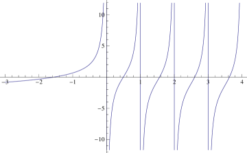
Figure 4.1. Graph of $G(\lambda)$, and a root between $-2$ and $-1$.

To finish verifying rigorously that this figure illustrates the behavior of $G$, it remains to show that there is a negative root; and to show $G(\lambda)\to-\infty$ as $\lambda\to-\infty.$

To see that there is root between $-1$ and $-2$ we calculate as follows:

$$G(-1) =\sum_{k=0}^{\infty}\frac{1-k}{\left(1+k\right)\left(1+k^{2}\right)}=1-\sum_{k=2}^{\infty}\frac{k-1}{\left(1+k\right)\left(1+k^{2}\right)}$$

$$G(-2) =\sum_{k=0}^{\infty}\frac{1-2k}{\left(2+k\right)\left(1+k^{2}\right)}=\frac{1}{2}-\sum_{k=1}^{\infty}\frac{2k-1}{\left(2+k\right)\left(1+k^{2}\right)}$$

hence

$$G(-1) >1-\sum_{k=2}^{\infty}\frac{k-1}{\left(1+k\right)\left(1+k^{2}\right)}=2-\frac{\pi\coth(\pi)}{2}\approx 0.423326$$

$$G(-2) <\frac{1}{2}-\left(\frac{1}{3\cdot 2}+\frac{3}{4\cdot 5}+\frac{5}{5\cdot 10}+\frac{7}{6\cdot 17}+\frac{9}{7\cdot 26}\right)=-\frac{215}{6188}.$$

Hence there is a root between $-2$ and $-1$, by the intermediate value theorem.

Finally, it remains to show that $G(\lambda)\to-\infty$ as $\lambda\to-\infty.$

Write

$$G(-\lambda) =\sum_{k=0}^{\infty}\frac{1-\lambda\,k}{\left(k+\lambda\right)\left(1+k^{2}\right)}$$

for $\lambda>0.$ Since

$$0\leq\sum_{k=0}^{\infty}\frac{1}{\left(k+\lambda\right)\left(1+k^{2}\right)}\leq\sum_{k=0}^{\infty}\frac{1}{k\left(1+k^{2}\right)}<\infty,$$

we need to show

$$\sum_{k=0}^{\infty}\frac{\lambda\,k}{\left(k+\lambda\right)\left(1+k^{2}\right)}\to\infty$$

as $\lambda\to\infty.$ Observe that

$$\frac{d}{d\lambda}\frac{\lambda\,k}{(k+\lambda)\left(1+k^{2}\right)}=\frac{k^{2}}{(k+\lambda)^{2}\left(1+k^{2}\right)}>0.$$

Hence by Monotone Convergence Theorem

$$\lim_{\lambda\to\infty}\sum_{k=0}^{\infty}\frac{\lambda\,k}{\left(k+\lambda\right)\left(1+k^{2}\right)} =\sum_{k=0}^{\infty}\lim_{\lambda\to\infty}\frac{\lambda\,k}{\left(k+\lambda\right)\left(1+k^{2}\right)}$$

$$=\sum_{k=0}^{\infty}\frac{k}{1+k^{2}}=\infty.$$

The convergence is logarithmic as illustrated by Figure 4.2.

Now fix $t$ such that $\cos(t)\neq-1.$ The intersection points in (4.10) can be constructed as follows:

The first coordinates of the intersection points of the horizontal line $y=\tan\left(t/2\right)$ and the curve $y=G(\lambda)$ are points

$$S(t):=\{\lambda_{n}(t)\}_{n\in\mathbb{N}_{0}}.$$ (4.12)

Each of the intervals $(-\infty,0)$, and $(n,n+1)$, $n=0,1,2,\ldots$ contains precisely one point from $S(t)$. Hence, the numbers in $S(t)$ from (4.12) can be assigned an indexing such that the monotone order relations in (4.9) are satisfied. ∎

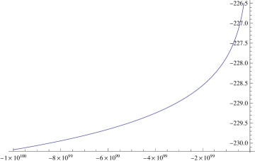
Figure 4.2. ${\displaystyle\lim_{\lambda\rightarrow-\infty}G(\lambda)=-\infty}$

Figure 4.3. The set $S(t)$ of intersection points.

Corollary 4.5.

For every $b<0$, there is a unique selfadjoint extension $H_{b}$ of $L$ such that $b$ is the bottom of the spectrum of $H_{b}$.

Corollary 4.6.

If $\zeta=e(t)\neq-1,$ $\lambda_{n}(t),$ $n=0,1,2,\ldots$ are the eigenvalues of $L_{t},$ and

$$y_{n,k}(t)=\frac{\lambda_{n}(t)}{k-\lambda_{n}(t)},\forall k\geq 0,$$ (4.13)

then $y_{n}(t)=\left(y_{n,k}(t)\right)_{k=0}^{\infty},$ $n=0,1,2,\ldots$ is an orthogonal basis for $\ell^{2}$; in particular,

$$\sum_{k\in\mathbb{N}_{0}}\frac{1}{\left(k-\lambda_{n}(t)\right)\left(k-\lambda_{m}(t)\right)}=0,\quad n\neq m.$$

Proof.

By Theorem 3.6 the spectrum of $L_{t}$ is discrete and has multiplicity one. By Theorem 4.4 no eigenvalue $\lambda_{n}(t)$ is an integer. By, the proof of, Lemma 3.4 the $y_{n}(t)$ are the eigenvectors for $L_{t}.$ ∎

Remark 4.7.

The norm of $y_{n}(t)$ can be evaluated in terms of gamma functions

$$\sum_{k=0}^{\infty}\left(\frac{\lambda_{n}(t)}{k-\lambda_{n}(t)}\right)^{2}=\lambda_{n}(t)^{2}\psi^{\prime}\left(-\lambda_{n}(t)\right)$$

where $\psi,$ known as the $\psi$ function, is the logarithmic derivative

$$\psi(t)=\frac{\Gamma^{\prime}(t)}{\Gamma(t)}$$

of the gamma function $\Gamma(t)=\int_{0}^{\infty}e^{-x}x^{t-1}dx.$ The derivatives of the $\psi$ function are called polygamma functions [ŞB11].

Theorem 4.8.

Let $t$ be fixed such that $\cos(t)\neq-1.$ Let $\lambda_{n}(t),$ $n\in\mathbb{N}_{0},$ be the eigenvalues of $L_{t}$ enumerated as in Theorem 4.4, then

$$n-\lambda_{n}(t)\to 0$$

as $n\to\infty.$

Proof.

The $\psi$ function has the series expansion [AS92],

$$\psi(z)=-\gamma+\sum_{k=0}^{\infty}\left(\frac{1}{k+1}-\frac{1}{k+z}\right),$$ (4.14)

where $\gamma$ is the Euler constant. Consequently, a computation shows that

$$G(\lambda) = \sum_{k\in\mathbb{N}_{0}}\frac{1+\lambda k}{\left(k-\lambda\right)\left(1+k^{2}\right)}$$ (4.15)

$$= \frac{1}{2}\left(\psi(i)+\psi(-i)-2\psi(-\lambda)\right)$$

$$= \Re\left(\psi(i)\right)-\psi(-\lambda).$$

Using this identity and (4.14) we find

$$G(\lambda)-G(\lambda-1) = G(\frac{1}{2})-G(-\frac{1}{2})+\int_{\frac{1}{2}}^{\lambda}\frac{d}{dx}\left(G(x)-G(x-1)\right)dx$$ (4.16)

$$= \sum_{k\in\mathbb{N}_{0}}\frac{1+\frac{1}{2}k}{\left(k-\frac{1}{2}\right)\left(1+k^{2}\right)}-\sum_{k\in\mathbb{N}_{0}}\frac{1-\frac{1}{2}k}{\left(k+\frac{1}{2}\right)\left(1+k^{2}\right)}$$

$$+\int_{\frac{1}{2}}^{\lambda}\left(\sum_{k\in\mathbb{N}_{0}}\frac{1}{\left(k-x\right)^{2}}-\sum_{k\in\mathbb{N}_{0}}\frac{1}{\left(k+1-x\right)^{2}}\right)dx$$

$$= \sum_{k\in\mathbb{N}_{0}}\frac{4}{4k^{2}-1}+\int_{\frac{1}{2}}^{\lambda}\frac{1}{x^{2}}\,dx$$

$$= -2+\left(2-\lambda^{-1}\right)=-\lambda^{-1}.$$

Caution. Note that in equating the two sides, it is understood that the common poles on the LHS have been cancelled, so only one contribution from a pole remains, from the pole at $\lambda=0$. While cancellation of poles is $\infty-\infty$, nonetheless, our assertion is precise because we verify agreement of the residues at the poles that are subtracted.

With this caution, we note that (4.15) and (4.16) extend to $\mathbb{C}$, i.e., that both equations now will be valid for all complex values of $\lambda$.

Hence, if $\lambda=n+\varepsilon$ with $n\geq 0$ and $0<\varepsilon<1,$ then

$$G(\lambda)=G(n+\varepsilon) =G(\varepsilon)-\frac{1}{1+\varepsilon}-\frac{1}{2+\varepsilon}-\cdots-\frac{1}{n+\varepsilon}$$

$$<G(\varepsilon)-\frac{1}{2}-\frac{1}{3}-\cdots-\frac{1}{n+1}.$$

Since $\sum_{k=2}^{\infty}1/k$ is divergent the result follows. ∎

Remark 4.9.

The proof of Theorem 4.8 shows, the graph of $G(\lambda),$ $n<\lambda<n+1$, is obtained from the graph of $G(\lambda),$ $n-1<\lambda<n,$ by shifting the point $(\lambda-1,G(\lambda-1))$ to the point $\left(\lambda,G(\lambda-1)-\tfrac{1}{\lambda}\right)$.

Lemma 4.10.

The function $\mathbb{C}\ni z\mapsto\psi(z)$ in (4.14) in Theorem 4.8 is meromorphic with simple poles at $z\in-\mathbb{N}_{0}$, all residues are $-1$; and $\psi(\cdot)$ is reflection symmetric, i.e., $\psi(\overline{z})=\overline{\psi(z)}$, $z\in\mathbb{C}$.

Moreover, for the two functions $\Re\{\psi\}$ and $\Im\{\psi\}$, we have the following formulas

$$\Re\{\psi(x+iy)\} = -\gamma+\sum_{k\in\mathbb{N}_{0}}\frac{(x-1)(x+k)+y^{2}}{\left(k+1\right)(\left(x+k\right)^{2}+y^{2})}$$ (4.17)

$$\Im\{\psi(x+iy)\} = \sum_{k\in\mathbb{N}_{0}}\frac{y}{\left(x+k\right)^{2}+y^{2}}$$ (4.18)

for all $x+iy\in\mathbb{C}$; where $\gamma$ is the Euler–Mascheroni constant. (Note the occurrence of the kernels of Poisson and of the Hilbert transform. Indeed, the formula (4.18) for $\Im\{\psi(z)\}$ is a sampling of the Poisson kernel for the upper half plane, sampled on the $x$-axis with points from $\mathbb{N}_{0}$ as sample points.)

In particular the numbers

$$\Re\{\psi(i)\} = -\gamma+\sum_{k\in\mathbb{N}_{0}}\frac{1-k}{\left(k+1\right)\left(k^{2}+1\right)}\thickapprox 0.0946503$$ (4.19)

$$\Im\{\psi(i)\} = \sum_{k\in\mathbb{N}_{0}}\frac{1}{k^{2}+1}=\frac{1}{2}\left(1+\pi\coth(\pi)\right)=K;$$ (4.20)

see (4.3).

Proof.

The first assertion in the lemma follows from (4.14) and the following reduction:

$$\psi(z)=-\gamma+(z-1)\sum_{k\in\mathbb{N}_{0}}\frac{1}{\left(k+z\right)\left(k+1\right)}.$$ (4.21)

Fix $n\in\mathbb{N}_{0}$; then

$$\lim_{z\rightarrow-n}(z+n)\psi(z)=-1.$$

From (4.14), we see that

$$\psi(x+iy) = -\gamma+\sum_{k\in\mathbb{N}_{0}}\left(\frac{1}{k+1}-\frac{1}{\left(x+k\right)+iy}\right)$$

$$= -\gamma+\sum_{k\in\mathbb{N}_{0}}\left(\frac{1}{k+1}-\frac{x+k}{\left(x+k\right)^{2}+y^{2}}\right)+i\sum_{k\in\mathbb{N}_{0}}\frac{y}{\left(x+k\right)^{2}+y^{2}}$$

$$= -\gamma+\sum_{k\in\mathbb{N}_{0}}\frac{(x-1)(x+k)+y^{2}}{\left(k+1\right)(\left(x+k\right)^{2}+y^{2})}+i\sum_{k\in\mathbb{N}_{0}}\frac{y}{\left(x+k\right)^{2}+y^{2}}.$$

The desired results follow from this.∎

Remark 4.11.

As a consequence of the Lemma 4.10, we get the following:

For every

$$v:=K\tan(\pi t)\in\mathbb{R},\;(\mbox{see }(\ref{eq:eeqn}))$$ (4.22)

and every $n\in\mathbb{N}$, let

$$\mathbb{D}_{v,n}:=\left\{z\in\mathbb{C}\>:\>\left|z-(n-\frac{1}{2})\right|<r_{n}\right\}$$

where $r_{n}\in(\frac{1}{2},1)$, and such that $G(z)-v$ has only one zero in $\mathbb{D}_{v,n}$. Then, by the argument principle,

$$\frac{1}{2\pi i}\oint_{\partial\mathbb{D}_{v,n}}\frac{zG^{\prime}(z)}{G(z)-v}dz = \sum(\mbox{zeros})-\sum(\mbox{poles})$$ (4.23)

$$= \lambda_{n}(t)-\left(2n-1\right).$$ (4.24)

See Figure 4.3. Therefore,

$$\lambda_{n}(t)=(2n-1)+\frac{1}{2\pi i}\oint_{\partial\mathbb{D}_{v,n}}\frac{zG^{\prime}(z)}{G(z)-v}dz,\quad n\in\mathbb{N}.$$ (4.25)

The proof of Theorem 4.4 shows that for each $n,$ $t\to\lambda_{n}(t)$ is a continuous function $\lambda_{n}:(-\pi,\pi)\to\mathbb{R},$ when $n\geq 1$ and $\lambda_{0}:(-\infty,0)\to\mathbb{R},$ such that

$$\lambda_{n}(t)\nearrow n \text{ as }t\nearrow\pi\,\,\,\,\,\,\,\,\,\,\text{for all }n\geq 0$$

$$\lambda_{n}(t)\searrow n-1 \text{ as }t\searrow-\pi\,\,\,\,\,\text{for all }n\geq 1,\text{ and}$$ (4.26)

$$\lambda_{0}(t)\searrow-\infty \text{ as }t\searrow-\pi.$$

The case $t=\pm\pi$ has spectrum $\mathbb{N}_{0}.$ In particular,

$$\bigcup_{\zeta\in\mathbb{T}}\mathrm{spectrum}\left(H_{\zeta}\right)=\bigcup_{t\in(-\pi,\pi]}\mathrm{spectrum}\left(L_{t}\right)=\mathbb{R}$$

and the unions are disjoint.

In the proof of Theorem 4.8 we saw that the $\lambda_{0}(t)\searrow-\infty\text{ as }t\searrow-\pi$ is logarithmic. The purpose of the next result is to establish rates of convergence for the remaining limits in (4.26).

Theorem 4.12.

Let $\lambda_{n}(t),$ $n\in\mathbb{N}_{0},$ be the eigenvalues of $L_{t}$ enumerated as in Theorem 4.4 and let $\gamma_{0}=2\gamma+\psi(i)+\psi(-i),$ where $\gamma$ is the Euler constant and $\psi$ is the digamma function, then $\gamma_{0}\approx-1.34373$ and for $-\pi<t<\pi$ we have

$$\lambda_{0}(t) \approx-\frac{\pi-t}{2K}-\frac{\gamma_{0}}{2}\left(\frac{\pi-t}{2K}\right)^{2},\text{ when }t\approx\pi$$

$$\lambda_{n}(t) \approx n-\frac{\pi-t}{2K}+\left(-\gamma_{0}+2\sum_{k=1}^{n}\frac{1}{k}\right)\left(\frac{\pi-t}{2K}\right)^{2},\text{ when }t\approx\pi$$

$$\lambda_{n+1}(t) \approx n+\frac{\pi+t}{2K}+\left(-\gamma_{0}+2\sum_{k=1}^{n}\frac{1}{k}\right)\left(\frac{\pi+t}{2K}\right)^{2},\text{ when $t\approx-\pi$}$$

for all $n\geq 1.$ Here $K=\tfrac{1}{2}\left(1+\pi\coth(\pi)\right)\approx 2.07667$.

Proof.

Recall, see Figure 4.4, when $-\pi<t<\pi,$ the eigenvalues of $L_{t}$ are the solutions $-\infty<\lambda_{0}(t)<0,$ and for $n\geq 1,$ $n-1<\lambda_{n}(t)<n$ to

$$G\left(\lambda_{n}(t)\right)=K\tan(t/2)$$ (4.27)

and

$$G(\lambda)=\sum_{k=0}^{\infty}\frac{1+\lambda k}{\left(k-\lambda\right)\left(1+k^{2}\right)} = \frac{1}{2}\left(\psi(i)+\psi(-i)-2\psi(-\lambda)\right)$$ (4.28)

$$= \Re\{\psi(i)\}-\psi(-\lambda).$$

Here

$$\psi(z)=-\gamma+\sum_{k=0}^{\infty}\frac{z-1}{(k+1)(k+z)}$$ (4.29)

is the digamma function and $\gamma$ is the Euler constant.

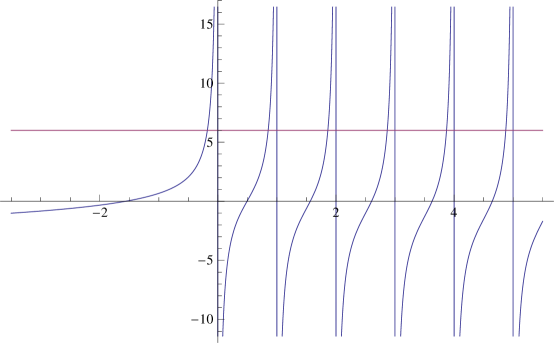
Figure 4.4. $G(\lambda),K\tan(t/2)=6$

Since we would like to find the asymptotics of $t\to\lambda_{n}(t)$ at the asymptotes, it is convenient to rewrite (4.27) as

$$g(\lambda)=\cot(t/2)/K,$$ (4.30)

where $g(\lambda)=1/G(\lambda)$ when $\lambda\notin\mathbb{N}_{0}$ and $g(\lambda)=0$ when $\lambda\in\mathbb{N}_{0}.$ Then $g$ is analytic in a neighborhood of $n$ for all $n\in\mathbb{N}_{0}.$ Note $\cot(t/2)\to 0$ as $t\to\pm\pi.$ Let $I_{n}$ be the open interval containing $n$ whose endpoints are roots of $G(\lambda)$ and let

$$h_{n}(x)=\left(g\mid_{I_{n}}\right)^{-1}(x).$$

For each $n\geq 0,$ $h_{n}$ is the inverse of a restriction of $g$ satisfying $h_{n}(0)=n.$

By construction of $h_{n}$ we can rewrite (4.30) as

$$h_{n}\left(\cot(t/2)/K\right)=\begin{cases}\lambda_{n+1}(t),&\text{when }0<t<\pi\\ \lambda_{n}(t),&\text{when }-\pi<t<0\end{cases},$$

for $n=0,1,2,\ldots$Hence, to investigate the asymptotics of $\lambda_{n}(t)$ as $t\nearrow\pi$ and as $t\searrow-\pi,$ we need to investigate the asymptotics of $h_{n}\left(\cot(t/2)/K\right)$ as $t\nearrow\pi$ and as $t\searrow-\pi.$ We will do this by writing down a few terms of the Taylor series at $0$ of $h_{n}$ for each $n.$

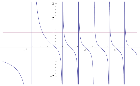
Figure 4.5. $g(\lambda)=1/G(\lambda),\cot(t/2)=K$

As noted above $h_{n}(0)=n.$ It is easy to see that

$$h_{n}^{\prime}(x) =\frac{1}{g^{\prime}\left(h_{n}(x)\right)}\text{ and}$$

$$h_{n}^{\prime\prime}(x) =-\frac{g^{\prime\prime}\left(h_{n}(x)\right)}{\left(g^{\prime}\left(h_{n}(x)\right)\right)^{3}}.$$

Hence, using that $h_{n}(0)=n,$ we see that to calculate the derivatives of $h_{n}(x),$ at $x=0,$ it is sufficient to calculate the derivatives

$$g^{\prime}(n),g^{\prime\prime}(n),\ldots.$$

Using (4.28) and $g(x)=1/G(x),$ we get $g(x)=2/\left(\psi(i)+\psi(-i)-2\psi(-x)\right),$ so

$$g^{\prime}(x) =\frac{-4\psi^{\prime}(-x)}{\left(\psi(i)+\psi(-i)-2\psi(-x)\right)^{2}}$$

$$=\frac{-\psi^{\prime}(x)}{\left(\Re\left\{\psi(i)\right\}-\psi(-x)\right)^{2}},$$ (4.31)

and

$$g^{\prime\prime}(x) = \frac{4\psi^{\prime\prime}(-x)\left(\psi(i)+\psi(-i)-2\psi(-x)\right)+16\left(\psi^{\prime}(-x)\right)^{2}}{\left(\psi(i)+\psi(-i)-2\psi(-x)\right)^{3}}.$$ (4.32)

$$= \frac{\psi^{\prime\prime}(-x)\left(\Re\{\psi(i)\}-\psi(-x)\right)+2\left(\psi^{\prime}(-x)\right)^{2}}{\left(\Re\left\{\psi(i)\right\}-\psi(-x)\right)^{3}}.$$

To calculate $\psi^{\prime\prime}(n)$ we need some more information of $\psi(x).$ By (4.14)

$$\psi(-x)=-\gamma+\frac{1}{x}+\sum_{k=1}^{\infty}\left(\frac{1}{k}-\frac{1}{k-x}\right).$$ (4.33)

Hence

$$\psi^{\prime}(-x)=\sum_{k=0}^{\infty}\frac{1}{(k-x)^{2}}\text{ and }\psi^{\prime\prime}(-x)=-2\sum_{k=0}^{\infty}\frac{1}{(k-x)^{3}}.$$ (4.34)

Plugging (4.33) and (4.34) into (4.31) we see that the numerator and denominator are meromorphic functions with poles of the same order at $x=n.$ It follows that

$$g^{\prime}(n)=-1,\text{ for all }n\geq 0.$$

Similarly, it follows from (4.33), (4.34), and (4.32) that

$$g^{\prime\prime}(0) =-2\gamma-\psi(i)-\psi(-i)=-\gamma_{0}$$

$$g^{\prime\prime}(n) =-\gamma_{0}+2\sum_{k=1}^{n}\frac{1}{k},\text{ for all }n\geq 1.$$

So that $h_{n}^{\prime}(0)=-1$ for all $n\geq 0,$ $h_{0}^{\prime\prime}(0)=-\gamma_{0},$ and $h^{\prime\prime}_{n}(0)=-\gamma_{0}+2\sum_{k=1}^{n}\frac{1}{k}.$ Hence,

$$\lambda_{0}(t)\approx-\frac{\cot(t/2)}{K}-\frac{\gamma_{0}}{2}\left(\frac{\cot(t/2)}{K}\right)^{2},\text{ when }t\approx\pi$$

and for all $n\geq 1,$

$$\lambda_{n}(t)\approx n-\frac{\cot(t/2)}{K}+\left(-\gamma_{0}+2\sum_{k=1}^{n}\frac{1}{k}\right)\left(\frac{\cot(t/2)}{K}\right)^{2}, t\approx\pi$$ when

$$\lambda_{n+1}(t)\approx n-\frac{\cot(t/2)}{K}+\left(-\gamma_{0}+2\sum_{k=1}^{n}\frac{1}{k}\right)\left(\frac{\cot(t/2)}{K}\right)^{2} t\approx-\pi.$$ when

Using

$$\cot(t/2) =\frac{\pi-t}{2}+\frac{\left(\pi-t\right)^{3}}{24}+\frac{\left(\pi-t\right)^{7}}{240}+O\left((\pi-t)^{7}\right)$$

$$=-\frac{\pi+t}{2}+\frac{\left(\pi+t\right)^{3}}{24}+\frac{\left(\pi+t\right)^{7}}{240}+O\left((\pi+t)^{7}\right),$$

completes the proof. ∎

5. Quadratic Forms

In this section we show that the basic Hermitian operator $L$ from section 3 has zero as its lower bound, i.e., that no positive number is a lower bound for $L$.

Let

$$Q_{L}(x)=\left\langle x,Lx\right\rangle=\sum_{k\in\mathbb{N}_{0}}k\left|x_{k}\right|^{2},\quad x\in\mathbb{D}_{0}.$$

Lemma 5.1.

The quadratic form $Q_{L}$ has greatest lower bound zero.

Proof.

Clearly, $Q_{L}(x)\geq 0$ for all $x\in\mathscr{D}(L)$. What is the largest constant $c$ such that

$$Q_{L}(x)\geq c\left\langle x,x\right\rangle,\quad x\in\mathscr{D}(L)\>?$$

Clearly, $c\geq 0.$

Next we will minimize

$$\sum_{k\in\mathbb{N}_{0}}k\left|x_{k}\right|^{2}$$

subject to the constraints

$$\sum_{k\in\mathbb{N}_{0}}\left|x_{k}\right|^{2}=1\text{ and }\sum_{k\in\mathbb{N}_{0}}x_{k}=0.$$ (5.1)

Indeed, we prove $\mbox{GLB}(L)=0$.

To do this, set ${\displaystyle s_{n}=\sum_{i=1}^{n}\frac{1}{i}}$, $n=1,2,.\dots$, and

$$x_{j}^{(n)}=\begin{cases}-s_{n}&\mbox{if }j=0\\ \frac{1}{j}&\mbox{if }1\leq j\leq n\\ 0&\mbox{if }j>n.\end{cases}$$

Note $(x^{(n)})\in\mathbb{D}_{0}=\mathscr{D}(L)$, for all $n$. Then

$$\frac{Q_{L}(x^{(n)})}{\left\|x^{(n)}\right\|_{2}^{2}} =\frac{\sum_{i=1}^{n}i\left(x_{i}^{(n)}\right)^{2}}{\left(\sum_{i=1}^{n}x_{i}^{(n)}\right)^{2}+\sum_{i=1}^{n}\left(x_{i}^{(n)}\right)^{2}}$$

$$=\frac{\sum_{i=1}^{n}\frac{1}{i}}{\left(\sum_{i=1}^{n}\frac{1}{i}\right)^{2}+\sum_{i=1}^{n}\frac{1}{i^{2}}}$$

$$=\frac{s_{n}}{\left(s_{n}\right)^{2}+\sum_{i=1}^{n}\frac{1}{i^{2}}}$$

$$\sim\frac{1}{s_{n}}\rightarrow 0.$$

Recall that

$$\lim_{n\rightarrow\infty}\sum_{i=1}^{n}\frac{1}{i} =\lim_{n\rightarrow\infty}s_{n}=\infty\;\mbox{and}$$

$$\lim_{n\rightarrow\infty}\sum_{i=1}^{n}\frac{1}{i^{2}} =\frac{\pi^{2}}{6}.$$

∎

5.1. Lower Bounds for Restrictions

The result from Lemma 5.1 in the present section, while dealing with an example, illustrates a more general question: Consider a selfadjoint operator $H$ in a Hilbert space $\mathscr{H}$ having its spectrum $spec(H)$ contained in the halfline $[0,\infty)$, and with $0\in spec(H)$. Then every densely defined Hermitian restriction $L$ of $H$ will define a quadratic form $Q_{L}$ also having $0$ as a lower bound. But, in general, the greatest lower bound (GLB) for such a restriction may well be strictly positive.

The particular restriction $L$ in Lemma 5.1 does have $\mbox{GLB}(Q_{L})=0$; and this coincidence of lower bounds will persist for a general family of cases to be considered in section 6.

Nonetheless, as we show below, there are other related semibounded selfadjoint operators $H$ with $0$ in the bottom of $spec(H)$, and having densely defined restrictions $L$ such that $\mbox{GLB}(Q_{L})$ is strictly positive. We now outline such a class of examples. The deficiency indices will be $(2,2)$.

We begin by specifying the selfadjoint operator $H$ and then identifying its restriction $L$. We do this by identifying $\mathscr{D}(L)$ as a subspace in $\mathscr{D}(H)$, still with $\mathscr{D}(L)$ dense in the ambient Hilbert space $\mathscr{H}$. But to analyze the operators we will have occasion to switch between two different ONBs. To do this, it will be convenient to realize vectors in $\mathscr{H}$ in cosine and sine-Fourier bases for $L^{2}(0,\pi)$. In this form, our operators may be specified as $-(d/dx)^{2}$ with suitable boundary conditions. The reason for the minus-sign is to make the operators semibounded.

But establishing the stated bounds is subtle, and inside the arguments, we will need to alternate between the two Fourier bases in $L^{2}(0,\pi)$. Indeed, inside the proof we switch between the two ONBs. This allows us to prove $\mbox{GLB}(Q_{L})=1$, i.e., establishing the best lower bound for the restriction $L$; strictly larger than the bound for $H$.

Hence vectors in our Hilbert space $\mathscr{H}$ will have equivalent presentations both the form of $l^{2}$ (square-summable sequences, one of each of the two orthogonal bases) and of $L^{2}(0,\pi)$. To get a cosine-Fourier representation for a function $f\in L^{2}(0,\pi)$, make an even extension $F_{ev}$ of $f$, i.e., extending $f$ to $(-\pi,\pi)$, then make a cosine-Fourier series for $F_{ev}$, and restrict it back to $(0,\pi)$. To get a sine-Fourier series for $f$, do the same but now using instead an odd extension $F_{odd}$ of $f$ to $(-\pi,\pi)$.

Let $\mathscr{H}^{(s)}:=l^{2}(\mathbb{N}_{0})$, with the standard basis

$$e_{k}=(0,\ldots,0,\underset{k^{th}}{1},0,\ldots),\quad k\in\mathbb{N}_{0}.$$ (5.2)

Let $H$ be the selfadjoint operator in $\mathscr{H}^{(s)}$ specified by

$$\mathscr{D}^{(s)}(H) = \left\{\alpha=(a_{n})\in l^{2}\>\big{|}\>\left(n^{2}a_{n}\right)\in l^{2},\;n\in\mathbb{N}_{0}\right\}$$ (5.3)

$$\left(H\alpha\right)_{n} = n^{2}a_{n},\;\forall\alpha\in\mathscr{D}(H).$$ (5.4)

In particular, $He_{0}=0$, and so $\inf\{spec(H)\}=0$.

Consider the restriction

$$L\subset H$$ (5.5)

with domain

$$\mathscr{D}_{1}^{(s)}:=\left\{\left(a_{n}\right)\in\mathscr{D}(H)\>\Big{|}\>\sum_{n=0}^{\infty}a_{2n}=\sum_{n=0}^{\infty}a_{2n+1}=0\right\}$$ (5.6)

Let $\mathscr{H}^{(c)}:=L^{2}(0,\pi)$. Using Fourier series, there is a natural isometric isomorphism

$$\mathscr{H}^{(s)}\simeq\mathscr{H}^{(c)},$$ (5.7)

corresponding to the two orthogonal bases in $L^{2}(0,\pi)$. Recall that, for all $f\in L^{2}(0,\pi)$,

$$f(x) = \sum_{n=0}^{\infty}a_{n}\cos(nx)$$ (5.8)

$$= \sum_{n=1}^{\infty}b_{n}\sin(nx).$$ (5.9)

Note that the two right-hand sides in (5.8) and (5.9) correspond to even and odd $2\pi$-periodic extensions of $f(x)$.

Remark 5.2.

In (5.6), $e_{0}\in\mathscr{D}(H)\backslash\mathscr{D}_{1}^{(s)}$. To see this, note that while the constant function $f_{0}\equiv 1/\sqrt{\pi}$ on $(0,\pi)$ has $e_{0}$ as its cos-representation via (5.8), its sin-representation $(b_{n})$ via (5.9) is as follows:

$$b_{n}=\begin{cases}\sqrt{\frac{3}{\pi}}\frac{1}{1+2k}&\mbox{ if }n=1+2k,\>\mbox{odd, and}\\ 0&\mbox{ if }n=2k,\>\mbox{even}.\end{cases}$$

Lemma 5.3.

Let $f\in L^{2}(0,\pi)$, and assume that $f^{\prime}$ and $f^{\prime\prime}\in L^{2}(0,\pi)$; then the combined boundary conditions

$$f=f^{\prime}=0\quad\mbox{at the two endpoints }x=0\mbox{ and }x=\pi$$ (5.10)

take the form

$$\sum_{n=0}^{\infty}a_{2n}=\sum_{n=0}^{\infty}a_{1+2n}=0$$ (5.11)

using the cos-representation (5.8), while in the sin-representation (5.9) for $f$, the same conditions (5.10) take the equivalent form:

$$\sum_{n=1}^{\infty}n\,b_{2n}=\sum_{n=0}^{\infty}(1+2n)b_{1+2n}=0.$$ (5.12)

Proof.

Direct substitution of (5.8) into (5.10) yields

$$\sum_{n\in\mathbb{N}_{0}}a_{n}=\sum_{n\in\mathbb{N}_{0}}(-1)^{n}a_{n}=0$$

which simplifies to (5.11). If instead we substitute (5.9) into (5.10), we get

$$\sum_{n\in\mathbb{N}}n\,b_{n}=\sum_{n\in\mathbb{N}}(-1)^{n}n\,b_{n}=0$$

which simplifies into (5.12).∎

Definition 5.4.

We set $\mathscr{D}\subset L^{2}(0,\pi)$ to be the dense subspace given by any one of the three equivalent systems of conditions (5.10), (5.11), and (5.12).

Lemma 5.5.

Let $\mathscr{H}=L^{2}(0,\pi)$ be as above, and let $\mathscr{D}$ be the dense subspace specified in Definition 5.4. We set

$$H=-\left(\frac{d}{dx}\right)^{2}\bigg{|}_{\left\{f\>\big{|}\>f=\sum_{n\in\mathbb{N}_{0}}a_{n}\cos(nx),\>(n^{2}a_{n})\in l^{2}\right\}}$$ (5.13)

i.e., restriction. (This is the Neumann-operator.)

It follows that $H$ is selfadjoint with spectrum $spec(H)=\left\{n^{2}\>\big{|}\>n\in\mathbb{N}_{0}\right\}$, and we set

$$L:=H\big{|}_{\mathscr{D}}.$$ (5.14)

Then $L$ is a densely defined restriction of $H$ and its deficiency indices are $(2,2)$.

Proof.

See Lemma 2.3 and the discussion above. Note that $\mathscr{D}$ arises from $\mathscr{D}(H)$ by imposition of the two additional linear conditions (5.11). Hence the deficiency indices are $(2,2)$.

Under (5.7), we have the following correspondence:

$$\mathscr{D}^{(s)} \longleftrightarrow \mathscr{D}^{(c)}:=\left\{f,f^{\prime\prime}\in\mathscr{H}^{(c)}\right\};$$

$$\mathscr{D}_{1}^{(s)} \longleftrightarrow \mathscr{D}_{1}^{(c)}:=\left\{f\in\mathscr{H}^{(c)}\>\big{|}\>f(0)=f(\pi)=0\right\}\,\,\,\,\,\,\,\,\,(\mbox{Dirichlet})$$

$$\mathscr{D}_{2}^{(s)} \longleftrightarrow \mathscr{D}_{2}^{(c)}:=\left\{f\in\mathscr{H}^{(c)}\>\big{|}\>f^{\prime}(0)=f^{\prime}(\pi)=0\right\}\,\,\,\,\,\,(\mbox{Neumann})$$

Moreover,

$$(H,\mathscr{D}^{(s)})\longleftrightarrow\left(-\left(d/dx\right)^{2},\mathscr{D}^{(c)}\right)\quad\mbox{selfadjoint}$$

and for the restriction operator,

$$(L,\mathscr{D})\longleftrightarrow(-\left(d/dx\right)^{2},\mathscr{D})$$

where $\mathscr{D}$ is the dense subspace in Definition 5.4. ∎

Lemma 5.6.

Let $(L,\mathscr{D})$ be the restriction of $H$ to $\mathscr{D}$. Then

$$\inf\left\{\frac{\left\langle\alpha,L\alpha\right\rangle_{2}}{\left\|\alpha\right\|_{2}^{2}}\>\Big{|}\>\alpha\in\mathscr{D}\right\}=1.$$ (5.15)

Proof.

For all $\alpha=(a_{n})\in\mathscr{D}^{(s)}$, let

$$f_{\alpha}(x):=\sum_{n=0}^{\infty}a_{n}\cos(nx)=\sum_{n=1}^{\infty}b_{n}\sin(nx)$$

where we have switched in $\mathscr{H}^{(c)}=L^{2}(0,\pi)$ from the cosine basis to sine basis, $\left(a_{n}\right)\mapsto\left(b_{n}\right)$. Then, for all $\alpha\in\mathscr{D}$, we have:

$$\left\langle\alpha,L\alpha\right\rangle_{l^{2}} = \left\langle f_{\alpha},-\left(d/dx\right)^{2}f_{\alpha}\right\rangle_{\mathscr{H}^{(c)}}$$ (5.16)

$$= \sum_{n=1}^{\infty}n^{2}\left|b_{n}\right|^{2}\geq\sum_{n=1}^{\infty}\left|b_{n}\right|^{2}=\left\|\alpha\right\|_{l^{2}}^{2}.$$

The desired result follows. ∎

Remark 5.7.

Note that (5.16) may be restated as a Poincaré inequality [AB09, YL11] as follows:

Let $f\in L^{2}(0,\pi)$ be such that $f^{\prime}$ and $f^{\prime\prime}$ are in $L^{2}$, and $f=f^{\prime}=0$ at the endpoints $x=0$, and $x=\pi$; then

$$\int_{0}^{\pi}\left|f^{\prime}(x)\right|^{2}dx\geq\int_{0}^{\pi}\left|f(x)\right|^{2}dx.$$ (5.17)

6. The Hardy space $\mathscr{H}_{2}$.

It is well known that there are two mirror-image versions of the basic $l^{2}$-Hilbert space $l^{2}(\mathbb{N}_{0})$ of one-sided square-summable sequences: On one side of the mirror we have plain $l^{2}(\mathbb{N}_{0})$, the discrete version; and on the other, there is the Hardy space $\mathscr{H}_{2}$ of functions $f(z)$, analytic in the open disk $\mathbb{D}$ in the complex plane, and represented with coefficients from $l^{2}(\mathbb{N}_{0})$. (See (6.1)-(6.2) below.) By “mirror-image” we are here referring to a familiar unitary equivalence between the two sides, see [Rud87]. This other viewpoint, involving complex power series, further makes useful connections to special function theory. In this connection, the following monographs [AS92, EMOT81] are especially relevant to our discussion below.

Introducing the analytic version $\mathscr{H}_{2}$ further allows us to bring to bear on our problem powerful tools from reproducing kernel theory, from harmonic analysis and analytic function theory (see e.g., [Rud87]). The reproducing kernel for $\mathscr{H}_{2}$ is the familiar Szegö kernel. This then further allows us to assign a geometric meaning to our boundary value problems, formulated initially in the language of von Neumann deficiency spaces. In the context of geometric measure theory, the reproducing kernel approach was used in [DJ11] in a related but different context.

Under the natural isometric isomorphism of $l^{2}$ onto $\mathscr{H}_{2}$, the domain $\mathscr{D}(H)$ in $l^{2}(\mathbb{N}_{0})$ is mapped into a subalgebra $\mathscr{A}(\mathscr{H}_{2})$ in $\mathscr{H}_{2}$, a Banach algebra, consisting of functions on the complex disk having continuous extensions to the closure of the disk $\overline{\mathbb{D}}$, and with absolutely convergent power series.

Lemma 6.1.

Under the isomorphism $l^{2}\simeq\mathscr{H}_{2}$, the selfadjoint operator $H$ becomes ${\displaystyle z\frac{d}{dz}}$, and the domain of its restriction $L$ consists of continuous functions $f$ on $\overline{\mathbb{D}}$, analytic in $\mathbb{D}$, $f\in\mathscr{A}(\mathscr{H}_{2})$, such that $f(1)=0$.

6.1. Domain Analysis

There is a natural isometric isomorphism $l^{2}(\mathbb{N}_{0})\simeq\mathscr{H}_{2}$ where $\mathscr{H}_{2}$ is the Hardy space of all analytic functions $f$ on $\mathbb{D}:=\{z\in\mathbb{C}\>\big{|}\>\left|z\right|<1\}$, with coefficients $(x_{k})\in l^{2}(\mathbb{N}_{0})$,

$$f(z)=\sum_{k=\mathbb{N}_{0}}x_{k}z^{k},$$ (6.1)

and where

$$\left\|f\right\|_{\mathscr{H}_{2}}^{2}=\sup_{r<1}\left\{\int_{0}^{1}\left|f(r\,e(t))\right|^{2}dt\right\};$$ (6.2)

see [Rud87]. (In (6.2), we used $e(t):=e^{i2\pi t}$, $t\in\mathbb{R}$.)

Lemma 6.2.

Under the unitary isomorphism $l^{2}(\mathbb{N}_{0})\simeq\mathscr{H}_{2}:x=(x_{k})\mapsto f(z)=\sum_{k\in\mathbb{N}_{0}}x_{k}z^{k}$, the selfadjoint operator $H:x\mapsto(k\,x_{k})$ becomes $f\mapsto z\frac{d}{dz}$, and

$$\mathscr{D}(H)\rightarrow\mathscr{A}(\mathscr{H}_{2})$$ (6.3)

where $\mathscr{A}(\mathscr{H}_{2})$ is the Banach algebra of functions $f\in\mathscr{H}_{2}$ with continuous extension $\tilde{f}$ to $\overline{\mathbb{D}}$.

The unitary one-parameter group $\{U(t)\}_{t\in\mathbb{R}}$ generated by $H=z\frac{d}{dz}$ in $\mathscr{H}_{2}$ is

$$\left(U(t)f\right)(z)=f\left(e(t)z\right),$$ (6.4)

for all $f\in\mathscr{H}_{2}$, $t\in\mathbb{R}$, and all $z\in\mathbb{D}$ (= the disk) where $e(t)=e^{i2\pi t}$.

Proof.

Since $\mathscr{D}(H)\subset l^{1}(\mathbb{N})$, the power series ${\displaystyle\tilde{f}(z)=\sum_{k\in\mathbb{N}}x_{k}z^{k}}$ is absolutely convergent for all $z\in\overline{\mathbb{D}}$ when $x\in\mathscr{D}(H)\subset l^{1}(\mathbb{N}_{0})$, but $f\mapsto\tilde{f}$ does not map onto $\mathscr{A}(\mathscr{H}_{2})$. ∎

Corollary 6.3.

The operators $\{U(t)\}_{t\in\mathbb{R}}$ in (6.4) extend to a contraction semigroup $\{U(t)\,;\,t\in\mathbb{C},\>t=s+i\sigma,\>\sigma>0\}$, i.e., analytic continuation in $t$ to the upper half-place $\mathbb{C}_{+}$, and

$$\left\|U(s+i\sigma)f\right\|_{\mathscr{H}_{2}}\leq\left\|f\right\|_{\mathscr{H}_{2}},\quad f\in\mathscr{H}_{2},$$

holds for all $s+i\sigma\in\mathbb{C}_{+}$.

Proof.

Follows from Lemma 6.1, and a substitution of $e(s+i\sigma)z$ into eq. (6.1) and (6.4).∎

Lemma 6.4.

Under the isomorphism ${\displaystyle x\rightarrow f(z)=\sum_{k\in\mathbb{N}_{0}}x_{k}z^{k}}$, the defect vector $y=\left(\frac{1}{1+k}\right)_{k\in\mathbb{N}_{0}}$ is mapped into

$$y(z)=-\frac{1}{z}\log\left(1-z\right),\;z\in\mathbb{D}\backslash\{0\}.$$ (6.5)

Under the isomorphism ${\displaystyle x\rightarrow f_{x}(z)=\sum_{k\in\mathbb{N}_{0}}x_{k}z^{k}}$, the domain $\mathscr{D}(L)$ of the restriction $L$ is

$$\left\{f\in\mathscr{H}_{2}\>\big{|}\>\left\langle y,\left(I+z\frac{d}{dz}\right)f\right\rangle_{\mathscr{H}_{2}}=0\right\}=\left\{\tilde{f}\in\mathscr{D}\widetilde{(H)}\>\big{|}\>\tilde{f}(1)=0\right\}.$$ (6.6)

Proof.

Immediate.∎

Theorem 6.5.

Let $\Phi$ be the Lerch’s transcendent [EMOT81, AS92],

$$\Phi(z,s,v)=\sum_{k\in\mathbb{N}_{0}}\frac{z^{k}}{\left(k+v\right)^{s}}.$$ (6.7)

(Recall that $\Phi$ converges absolutely for all $v\neq 0,-1,-2,\ldots$, with either $z\in\mathbb{D}$, or $z\in\partial\mathbb{D}=\mathbb{T}$ and $\Re(s)>1$. )

Under the isomorphism $l^{2}(\mathbb{N}_{0})\simeq\mathscr{H}_{2}$, the defect vectors ${\displaystyle\left(\frac{1}{k\mp i}\right)_{k\in\mathbb{N}_{0}}}$ in (3.5) are mapped to

$$\tilde{x}_{\pm}(z)=\Phi(z,1,\mp i);$$ (6.8)

and eq. (6.5) can be written as

$$y(z)=\Phi(z,1,1).$$ (6.9)

Moreover, the eigenvectors $\left(\frac{\lambda_{n}(t)}{k-\lambda_{n}(t)}\right)_{k\in\mathbb{N}_{0}}$in (4.13) are mapped to

$$\tilde{y}_{n,t}(z)=\lambda_{n}(t)\,\Phi(z,1,-\lambda_{n}(t)).$$

Hence, for all $t\in\mathbb{R}$, the set $\{\tilde{y}_{n,t}\}_{n\in\mathbb{N}_{0}}$ forms an orthogonal basis for $\mathscr{H}_{2}$.

Proof.

Follows from Lemma 6.1, Theorems 4.1 and 4.4. ∎

6.2. The Szegö Kernel

In understanding the defect spaces $\mathscr{D}_{\pm}$, and the partial isometries between them, we will be making use of the Szegö kernel. It is the reproducing kernel for the Hardy space $\mathscr{H}_{2}$, i.e., a function $K$ on $\mathbb{D}\times\mathbb{D}$ such $K(\cdot,z)\in\mathscr{H}_{2}$, $z\in\mathbb{D}$; and

$$f(z)=\left\langle K(\cdot,z),f\right\rangle_{\mathscr{H}_{2}},\quad f\in\mathscr{H}_{2}.$$ (6.10)

(Note our inner product is linear in the second variable.)

The following formula is known

$$K(w,z)=\frac{1}{1-\overline{z}w}.$$ (6.11)

Our main concern is properties of functions $f\in\mathscr{H}_{2}$ on the boundary $\partial\mathbb{D}$.

Lemma 6.6.

The following offers a correspondence between the two representations $l^{2}(\mathbb{N}_{0})$ and $\mathscr{H}_{2}$, see (6.1)-(6.2). Consider the two operators $L$ and $H$ from sections 3-4. In the $\mathscr{H}_{2}$ model, we have $H=z\frac{d}{dz}$ , $L=H\big{|}_{\mathscr{D}(L)}$, and

$$\mathscr{D}(L)=\{f\in\mathscr{H}_{2}\>\big{|}\>\tilde{f}(1)=0\}$$

where $\tilde{f}$ is the boundary function (see [Rud87, ch11]), i.e., for $e(x)\in\mathbb{T}=\partial\mathbb{D}$, a.a. $x\in\mathbb{R}/\mathbb{Z}\simeq[0,1)$, setting $e(x):=e^{i2\pi x}$, Fatou’s theorem states existence a.e. of the function $\tilde{f}$ as follows:

$$\tilde{f}(x)=\lim_{z\rightarrow e(x)}f(z).\quad(\mbox{non-tangentially})$$ (6.12)

We make the identification $\tilde{f}(e(x))\simeq\tilde{f}(x)$ with $\tilde{f}$ $\mathbb{Z}$-periodic. Under the correspondence: $f\longleftrightarrow\tilde{f}$, we have

$$f(z)=\int_{0}^{1}\frac{\tilde{f}(x)}{1-\overline{e(x)}z}dx$$ (6.13)

where the RHS in (6.13) is a Szegö -kernel integral. Moreover,

$$z\frac{d}{dz}f\longleftrightarrow\frac{1}{2\pi i}\frac{d}{dx}\tilde{f}.$$ (6.14)

As a result, for the vectors in the two defect-spaces $\mathscr{D}_{\pm}$ in Lemma 1.1, we have

$$f_{+}(z) = \int_{0}^{1}\frac{e^{-2\pi x}}{1-\overline{e(x)}z}dx$$

$$= \frac{1-e^{-2\pi}}{2\pi i}\sum_{n=0}^{\infty}\frac{z^{n}}{n-i},\;\mbox{ and}$$

$$f_{-}(z) = \int_{0}^{1}\frac{e^{2\pi x}}{1-\overline{e(x)}z}dx$$

$$= -\frac{e^{2\pi}-1}{2\pi i}\sum_{n=0}^{\infty}\frac{z^{n}}{n+i}.$$

Proof.

The key ingredient in the proof is the representation of $f(z)\in\mathscr{H}_{2}$ as kernel integrals arising from the corresponding boundary versions $\tilde{f}(x)\simeq\tilde{f}(e(x))$ where $e(x)=e^{i2\pi x}$, and $\tilde{f}$ is as in (6.12). The kernel integral in (6.13) is a reproducing property for the Szegö-kernel, see [Rud87].

To show that the transform $f(z)\longleftrightarrow\tilde{f}(x)$ (Fatou a.e. extension to $\partial\mathbb{D}$) is a norm-preserving isomorphism of $\mathscr{H}_{2}$ onto a closed subspace in $L^{2}(\mbox{of a periodic interval})$, we check that

$$f(z)=\sum_{n=0}^{\infty}c_{n}z^{n}$$ (6.15)

where the coefficients $(c_{n})$ in (6.19) are also the Fourier-coefficients of the function $\tilde{f}$ in (6.12). But for $z\in\mathbb{D}$, i.e., $\left|z\right|<1$, we may expand the RHS in (6.13) as follows

$$f(z)=\sum_{n=0}^{\infty}z^{n}\int_{0}^{1}e(-nx)\tilde{f}(x)dx.$$

But

$$c_{n}=\int_{0}^{1}\overline{e(nx)}\tilde{f}(x)dx$$ (6.16)

are the $\tilde{f}$-Fourier coefficients over the period interval $[0,1)$. The result follows from this as follows

$$\left\|f\right\|_{\mathscr{H}_{2}}^{2} = \sum_{n=0}^{\infty}\left|c_{n}\right|^{2}\,\,\,\,\,\,\,\,\,\,\,\,\,\,\,\,\,\,\,(\mbox{by Lemma \ref{lem:H2}})$$

$$= \int_{0}^{1}\left|\tilde{f}(x)\right|^{2}dx\,\,\,\,\,\,\,(\mbox{by (}\ref{eq:cn}\mbox{) and Parseval applied to }\tilde{f})$$

$$= \left\|\tilde{f}\right\|_{L^{2}(0,1)}^{2}.$$

∎

Let ${\displaystyle H=z\frac{d}{dz}}$ be the selfadjoint operator in Lemma 6.1.

Corollary 6.7.

Under the boundary correspondence (6.12)-(6.13) in Lemma 6.6, if $f\in\mathscr{D}(H)\subset\mathscr{H}_{2}$; then the boundary function $\tilde{f}$ is a well-defined and continuous function on $\mathbb{T}\simeq[0,1)\simeq\mathbb{R}/\mathbb{Z}$. If further $f\in\mathscr{D}(H^{2})$, then $\tilde{f}$ ($=$ the boundary function) is Lipschitz, i.e.,

$$\left|\tilde{f}(x)-\tilde{f}(y)\right|\leq\mbox{Const}\cdot\left|x-y\right|.$$ (6.17)

Proof.

By Lemma 6.6 and Conclusions 6.11, the operator

$$\mathscr{H}_{2}\ni f\mapsto\tilde{f}\in\mathscr{L}_{+}\subset L^{2}(\mathbb{T})$$ (6.18)

is an isometric isomorphism of $\mathscr{H}_{2}$ onto $\mathscr{L}_{+}$. Moreover, see the proof of Lemma 6.6, if $f\in\mathscr{D}(H)$, then

$$\tilde{f}(e(x))=\sum_{n\in\mathbb{N}_{0}}c_{n}e(nx),\quad x\in\mathbb{R}/\mathbb{Z}$$ (6.19)

with $(c_{n})\in l^{2}$ and $(nc_{n})\in l^{2}$, see eq. (6.15)-(6.16). Hence $(c_{n})$ in (6.19) is in $l^{1}$, by Cauchy-Schwarz, see Lemma 3.1. Therefore, by domination, the boundary function $\tilde{f}$ in (6.19) is uniformly continuous on $\mathbb{T}$.

Assume now that $f\in\mathscr{D}(H^{2})$; then $(n^{2}c_{n})\in l^{2}$, and therefore:

$$\left|\tilde{f}(x)-\tilde{f}(y)\right| \leq \left|x-y\right|2\pi\sum_{n=1}^{\infty}\left|n\,c_{n}\right|$$

$$\leq \left|x-y\right|2\pi\left(\frac{\pi^{2}}{6}\right)^{1/2}\left(\sum_{n=1}^{\infty}n^{4}\left|c_{n}\right|^{2}\right)^{1/2}$$

$$\leq \left|x-y\right|\frac{2\pi^{2}}{\sqrt{6}}\left\|H^{2}f\right\|_{\mathscr{H}_{2}},$$

which is the desired Lipschitz estimate (6.17).∎

Corollary 6.8.

Consider the selfadjoint operator $H=z\,\frac{d}{dz}$ in $\mathscr{H}_{2}$ (as in Lemma 6.2). For $f\in\mathscr{D}(H^{2})$, consider the boundary function $\tilde{f}$ as in Lemma 6.6, and set

$$\mathscr{D}_{\{\pm 1\}}:=\left\{f\in\mathscr{D}(H^{2})\>\big{|}\>\tilde{f}(1)=\tilde{f}(-1)=0\right\}$$ (6.20)

and set

$$L_{2}:=H^{2}\bigg{|}_{\mathscr{D}_{\{\pm 1\}}},$$ (6.21)

then $L_{2}$ is a densely defined restriction of $H^{2}$, and

$$\mbox{GLB}(Q_{L_{2}})=1.$$ (6.22)

Proof.

An inspection shows that this example is unitarily equivalent to the one considered in Lemmas 5.3 and 5.5. Indeed, if $f\in\mathscr{D}(H^{2})$ has the representation $f(z)=\sum_{n\in\mathbb{N}_{0}}a_{n}z^{n}$, then the two conditions in (6.20) translate into

$$\sum_{n\in\mathbb{N}_{0}}a_{n}=\sum_{n\in\mathbb{N}_{0}}(-1)^{n}a_{n}=0;$$

or equivalently,

$$\sum_{n\in\mathbb{N}_{0}}a_{2n}=\sum_{n\in\mathbb{N}_{0}}a_{1+2n}=0;$$

compare with (5.11). Hence the result follows from Lemma 5.5.∎

Remark 6.9.

In using the unit-interval $I=[0,1]$ as range of the independent variable $x$ in the representation $\mathscr{H}_{2}\ni f(z)\longleftrightarrow\tilde{f}(x)$ via (6.12) we use the parameterization

$$I\ni x\mapsto e(x)=e^{i2\pi x}\in\mathbb{T}=\partial\mathbb{D}.$$ (6.23)

To justify the correspondence $\tilde{f}(x)\longleftrightarrow\tilde{f}(e(x))$ for a function $\tilde{f}$ on $\mathbb{R}$, as in $\tilde{f}=e^{-2\pi x}$, or $e^{2\pi x}$, it is understood that we use $1$-periodic versions of these functions, see Figure 6.1 and 6.2 below

Figure 6.1. Periodic version of $e^{-2\pi x}$

Figure 6.2. Periodic version of $e^{2\pi x}$

WARNING The role of the periodization (illustrated in Figures 6.1-6.2, and in (6.23)) is important. Indeed, if the period-interval used in Figs 1-2 is changed from $[0,1)$ into $[-\frac{1}{2},\frac{1}{2})$, we get the following related function $\tilde{y}_{2}(x)=e^{-2\pi\left|x\right|}$; see also Figure 6.3 below:

Figure 6.3. Periodic version of $e^{-2\pi\left|x\right|}$, periodic-interval $[-\frac{1}{2},\frac{1}{2})$

and

$$y_{2}(z) = \int_{-\frac{1}{2}}^{\frac{1}{2}}\frac{e^{-2\pi\left|x\right|}}{1-\overline{e(x)}z}dx$$ (6.24)

$$= \frac{1}{\left(2\pi\right)^{2}}\sum_{n=0}^{\infty}\frac{z^{n}}{1+n^{2}};$$

and we recovers the $l^{2}(\mathbb{N}_{0})$-sequence ${\displaystyle(y_{2})_{n}:=\frac{1}{1+n^{2}}}$ used in sections 3-4 above.

Remark 6.10.

In the isometric realization from Lemma 6.6 of the Hardy space $\mathscr{H}_{2}$ as a closed subspace inside $L^{2}(I)$ we are selecting a specific a period interval $I$. Avoiding a choice, an alternative to $L^{2}(I)$ is the Hilbert space $L^{2}(\mathbb{R}/\mathbb{Z})$ where the quotient group $\mathbb{R}/\mathbb{Z}$ is given its invariant quotient measure on $\mathbb{R}/\mathbb{Z}$. With the identification of $\mathbb{R}/\mathbb{Z}$ with $\mathbb{T}=\partial\mathbb{D}$, this is Haar measure on the one-torus $\mathbb{T}$. Of these three equivalent versions of Hilbert space, perhaps $L^{2}(\mathbb{R}/\mathbb{Z})$ is more natural as it doesn’t presuppose a choice of period interval.

The closed subspace $\mathscr{L}_{+}$ in $L^{2}(\mathbb{R}/\mathbb{Z})$ corresponding to $\mathscr{H}_{2}$ under (6.12) in Lemma 6.6 is of course the subspace of $L^{2}$ functions that have their Fourier coefficients vanish on the negative part of $\mathbb{Z}$. This subspace $\mathscr{L}_{+}$ in $L^{2}(\mathbb{R}/\mathbb{Z})$ is invariant under periodic translation $(U(t)f)(x)=f(x+t)$. Indeed this unitary one-parameter group $U(t)$, acting in $\mathscr{L}_{+}$, has as its infinitesimal generator our standard selfadjoint operator $H$ from Lemmas 3.1 and 6.6. Note that the spectrum of $H$ is $\mathbb{N}_{0}$ when $H$ is realized as a selfadjoint operator in $\mathscr{L}_{+}$; not in $L^{2}(\mathbb{R}/\mathbb{Z})$. One can adapt this approach in order to get realizations of the other selfadjoint extensions of $L$, and their associated unitary one-parameter groups.

Remark 6.11.

Conclusions (Toeplitz operators). In our study of selfadjoint extensions, we are making use of three (unitarily equivalent) realizations of Toeplitz operators; taking here “Toeplitz operator” to mean “matrix corner” of an operator in an ambient $L^{2}$ space, i.e., restriction of an operator $T$ in ambient $L^{2}$, followed by the projection $P$ onto the subspace; in short, $PTP$.

But it is helpful to realize these “matrix corners” in any one of three equivalent ways; hence three equivalent ways of realizing operators $T$ in the ambient Hilbert space and $PTP$ in its closed subspace:

1. realize the subspace as $\mathscr{L}_{+}$ inside $L^{2}(\mathbb{R}/\mathbb{Z})$, where $\mathscr{L}_{+}$ is the subspace of $L^{2}$-functions with vanishing negative Fourier coefficients;

2. or we may take the subspace to be the Hardy space $\mathscr{H}_{2}$ inside $L^{2}(\mathbb{T})$. Or equivalently,

3. we can work with the subspace of one-sided $l^{2}$ sequences inside two-sided; so the subspace $l^{2}(\mathbb{N}_{0})$ inside $l^{2}(\mathbb{Z})$.

So there are these three different but unitarily equivalent formulations; each one brings to light useful properties of the operators under consideration.

One detail which makes the analysis more difficult here as compared with the more classical case of $L^{2}$ is the study of unitary one-parameter groups: for example, periodic translation, $U(t):f\mapsto f(x+t)$, leaves invariant the subspace; but the related quasi-periodic translation does not.

ambient Hilbert space	closed subspace	$\mathscr{D}(H)$	$\mathscr{D}(L)$	$\mathscr{D}(L^{*})$
case 1 $l^{2}(\mathbb{Z})$	$l^{2}(\mathbb{N}_{0})$	$x\in l^{2}(\mathbb{N}_{0})$ s.t. $(k\,x_{k})\in l^{2}$	$x\in\mathscr{D}(H)$ s.t. $\sum_{k}x_{k}=0$	$\mathscr{D}(H)+\mathbb{C}y_{3}$
case 2 $L^{2}(\mathbb{T})$	$\mathscr{H}_{2}(\mathbb{D})$ (Hardy space)	$f\in\mathscr{H}_{2}$
s.t.
$z\frac{d}{dz}f\in\mathscr{H}_{2}$	$f\in\mathscr{D}(H)$ s.t.
$\tilde{f}(1)=0$	$\mathscr{D}(H)+\mathbb{C}\tilde{y}_{3}$
case 3 $L^{2}(\mathbb{R}/\mathbb{Z})$
$\simeq$
$L^{2}(I)$ $I=[0,1)$	$\mathscr{L}_{+}=\{f\in L^{2}\>\big{|}\>\hat{f}(n)=0,\>n\in\mathbb{Z}_{-}\}$	$f\in\mathscr{L}_{+}$
s.t. $\frac{d}{dx}f\in L^{2}$	$f\in\mathscr{D}(H)$ s.t. $f(0)=f(1)=0$	$\mathscr{D}(H)+\mathbb{C}P_{\mathscr{L}_{+}}\psi$, $\psi(x)=$
$\begin{cases}1&0\leq x<\frac{1}{2}\\ -1&\frac{1}{2}\leq x<1\end{cases}$

Table 1. Three models of Toeplitz operator analysis.

Remark 6.12.

In our model, we have $L\subset H\subset L^{*}$ (see (3.4)). As a result of (3.7), (3.8) and Remark 3.5, we see that

$$\dim\mathscr{D}(H)/\mathscr{D}(L)=\dim\mathscr{D}(L^{*})/\mathscr{D}(H)=1$$ (6.25)

(the two quotients are both one-dimensional); hence

$$\mathscr{D}(L^{*})=\mathscr{D}(H)+\mathbb{C}P_{\mathscr{L}_{+}}\psi.$$ (6.26)

The choice of the generating vector $\psi$ is not unique. For example, let $T$ be the triangular wave, i.e.,

$$T(x)=\frac{1}{2}-\left|x\right|,\quad x\in[-\frac{1}{2},\frac{1}{2}];$$ (6.27)

which has Fourier series

$$T(x)=\frac{1}{4}+\frac{2}{\pi^{2}}\sum_{n=1}^{\infty}\frac{1}{(2n-1)^{2}}\cos(2\pi(2n-1)x),\quad x\in[-\frac{1}{2},\frac{1}{2}].$$ (6.28)

Differentiating (6.27), we get the Haar wavelet $\psi$ as in Table 1; and where

$$\psi(x)=-\frac{4}{\pi}\sum_{n=1}^{\infty}\frac{1}{2n-1}\sin(2\pi(2n-1)x),\quad x\in(-\frac{1}{2},\frac{1}{2}).$$ (6.29)

It follows that

$$\left(P_{\mathscr{L}_{+}}\psi\right)(x)=\frac{2i}{\pi}\sum_{n=1}^{\infty}\frac{1}{2n-1}\,e_{2n-1}(x).$$ (6.30)

Note the Fourier coefficients satisfy

$$\left(\left(P_{\mathscr{L}_{+}}\psi\right)^{\wedge}(n)\right)\in l^{2}(\mathbb{N}_{0})$$

but

$$\left(n\left(P_{\mathscr{L}_{+}}\psi\right)^{\wedge}(n)\right)\notin l^{2}(\mathbb{N}_{0}).$$

6.3. $\mathscr{D}_{\pm}(L_{F})$ as RKHSs

For a fixed closed subset $F$ of $\partial\mathbb{D}$ of zero angular measure, we identified in Corollary 6.14 an associated Hermitian operator $L_{F}$ with dense domain in the Hardy space $\mathscr{H}_{2}$, see (6.33) and (6.34). Below we compute the corresponding pair of deficiency subspaces (see Lemma 1.2). While they are closed subspaces in $\mathscr{H}_{2}$, it turns out that they can be computed with reference to only the given closed set $F$. To this end we show in Theorem 6.18 that each deficiency subspace is a reproducing kernel Hilbert space (RKHS) with a positive definite kernel function on $F\times F$. The kernel is not the Szegö kernel, but rather the Hurwitz zeta function computed on differences of points in $F$ (angular variables), see (6.47) below. From this we show that the partial isometries between the two deficiency spaces "is" a compact group $G(F)$, a Lie group if $F$ is finite. With this, we prove in Corollary 6.26 a formula for the spectrum of each of the selfadjoint extensions of $L_{F}$.

Corollary 6.13.

Let $z_{1},z_{2},\ldots,z_{n}$ be a finite set of distinct points $\in\mathbb{C}$ s.t. $|z_{i}|=1$, $1\leq i\leq n$; and set

$$\mathscr{D}_{\{z_{i}\}}=\{f\in\mathscr{D}\widetilde{(H)}\>\big{|}\>\tilde{f}(z_{i})=0,\,1\leq i\leq n\};$$ (6.31)

then

$$L_{n}:=z\frac{d}{dz}\big{|}_{\mathscr{D}_{\{z_{i}\}}}$$ (6.32)

is Hermitian with dense domain in $\mathscr{H}_{2}$, and with deficiency indices $(n,n)$.

Proof.

This is an application of Lemma 2.3.∎

Corollary 6.14.

Let $F\subset\mathbb{T}=\{z\in\mathbb{C}\>\big{|}\>|z|=1\}=\partial\mathbb{D}$ be a closed subset of zero Haar measure, e.g., some fixed Cantor subset of $\mathbb{T}$; and set

$$\mathscr{D}_{F}:=\{f\in\mathscr{D}_{\mathscr{H}_{2}}(z\frac{d}{dz})\>\big{|}\>f=0\>\mbox{ on }F\},$$ (6.33)

then

$$L_{F}:=z\frac{d}{dz}\big{|}_{\mathscr{D}(F)}$$ (6.34)

is Hermitian with dense domain in the Hardy space $\mathscr{H}_{2}$, and with deficiency indices $(\infty,\infty)$.

Proof.

Follows again from the general result in Lemma 2.3. Since $F$ has Haar measure $0$, one verifies that the closed subspace $\mathfrak{M}$ in $\mathscr{H}_{2}$ defined for $\mathscr{D}_{F}$ in (6.33) (via Lemma 2.3) is closed in $\mathscr{H}_{2}$ and satisfies

$$\mathfrak{M}\cap\mathscr{D}(z\frac{d}{dz})=0.$$ (6.35)

∎

Remark 6.15.

Let $\mathscr{A}(\mathscr{H}_{2})$ be the Banach algebra introduced in Lemma 6.2, and let $F\subset\mathbb{T}$ be a closed subset specified as in Corollary 6.14. Let $L_{F}$ be the Hermitian restriction operator in (6.34), and $L_{F}^{*}$ its adjoint operator. Then both domains $\mathscr{D}(L_{F})$ and $\mathscr{D}(L_{F}^{*})$ are invariant under pointwise multiplication by functions $a$ from $\mathscr{A}(\mathscr{H}_{2})$, i.e.,

$$\left(af\right)(z)=a(z)f(z),\quad a\in\mathscr{A}(\mathscr{H}_{2}),\>f\in\mathscr{H}_{2},\>\mbox{and }z\in\mathbb{D}.$$ (6.36)

Hence this action of $\mathscr{A}(\mathscr{H}_{2})$ passes to the quotient

$$\mathscr{D}(L_{F}^{*})/\mathscr{D}(L_{F})\simeq\mathscr{D}_{+}(L_{F})+\mathscr{D}_{-}(L_{F}).$$ (6.37)

Corollary 6.16.

Let $F\subset\mathbb{T}$ be a closed subset of zero measure, see Corollary 6.14 and (6.33). Let $x_{\pm}\in l^{2}(\mathbb{N}_{0})$ be the sequences from (3.5), i.e., $x_{\pm}(k)=(k\mp i)^{-1}$, $k\in\mathbb{N}_{0}$. Then the two deficiency subspaces in $\mathscr{H}_{2}$ derived from (6.34)

$$\mathscr{D}_{\pm}(L_{F})=\{f_{\pm}\in\mathscr{D}(L_{F}^{*})\>\big{|}\>L_{F}^{*}f_{\pm}=\pm if_{\pm}\}$$ (6.38)

are as follows: For $\theta\in F$, set

$$f_{\pm}^{(\theta)}(z):=\sum_{n=0}^{\infty}\frac{e(-n\,\theta)}{n\mp i}z^{n};$$ (6.39)

i.e., the expansion coefficients for $f_{\pm}^{(\theta)}$ are

$$\widehat{f_{\pm}^{(\theta)}}(n)=\overline{e(n\,\theta)}\,x_{\pm}(n),\quad n\in\mathbb{N}_{0}.$$ (6.40)

Then $\mathscr{D}_{\pm}(L_{F})$ is the closed span in $\mathscr{H}_{2}$ of the functions in (6.39), as $\theta$ ranges over $F$.

Proof.

We will do the detailed steps for any $\{f_{+}^{(\theta)}(\cdot)\>\big{|}\>\theta\in F\}\subset\mathscr{D}_{+}(L_{F})$, as the other case for $\mathscr{D}_{-}(L_{F})$ is the same argument, mutatis mutandis.

Note that functions $\varphi\in\mathscr{D}(L_{F})$ are given by the condition

$$\varphi(\theta)\simeq\varphi(e(\theta))=0,\quad\forall\theta\in F$$ (6.41)

where we use the usual identification $\theta\longleftrightarrow e(\theta)=e^{i2\pi\theta}$ with points in a period interval $\simeq$ points in $\mathbb{T}$. For $\varphi\in\mathscr{D}(L_{F})$, set $x_{n}=\hat{\varphi}(n)$, i.e., ${\displaystyle\varphi(z)=\sum_{n\in\mathbb{N}_{0}}x_{n}z^{n}}$. Then for $\theta\in F$, we have; $(n\,x_{n})\in l^{2}(\mathbb{N}_{0})$, and:

$$0=\varphi(\theta) =\sum_{n=0}^{\infty}x_{n}e(n\,\theta)$$

$$=\left\langle\frac{\overline{e(n\,\theta)}}{n-i},(n+i)x_{n}\right\rangle_{l^{2}(\mathbb{N}_{0})}$$

$$=\left\langle f_{+}^{(\theta)},(L_{F}+iI)\varphi\right\rangle_{\mathscr{H}_{2}}$$ (6.42)

where, in the last step, we used the isomorphism $l^{2}(\mathbb{N}_{0})\simeq\mathscr{H}_{2}$ of Lemma 6.2. The respective subscripts $\left\langle\cdot,\cdot\right\rangle_{l^{2}(\mathbb{N}_{0})}$ and $\left\langle\cdot,\cdot\right\rangle_{\mathscr{H}_{2}}$ indicates the reference Hilbert space used.

Since (6.42) holds for all $\theta\in F$, it follows that each $f_{+}^{(\theta)}\in\mathscr{D}(L_{F})$, so the asserted “$=$” in the Corollary follows. ∎

Remark 6.17.

If $\theta\mbox{ and }\rho\in I$ ($=$ the period interval), then the $\mathscr{H}_{2}$-inner product of the two functions $f_{+}^{(\theta)}$ and $f_{-}^{(\theta)}$ is as follows:

$$\left\langle f_{+}^{(\theta)},f_{+}^{(\rho)}\right\rangle_{\mathscr{H}_{2}}=\sum_{n=0}^{\infty}\frac{e(n(\theta-\rho))}{1+n^{2}}=Z(\theta-\rho,1,2)$$ (6.43)

where $Z$ is the Hurwitz-zeta function.

Theorem 6.18.

Let the closed subset $F\subset\mathbb{T}$ be as in Corollary 6.16 and let $L_{F}$ be the corresponding Hermitian unbounded and densely defined operator in the Hardy space $\mathscr{H}_{2}$. Then each of the two defect spaces $\mathscr{D}_{\pm}(L_{F})$ in (6.38) is a reproducing kernel Hilbert space (RKHS) with RK equal to the Hurwitz zeta function (6.43).

Proof.

For the theory of RKHS, see for example [Nel57, Alp92, ABK02]. In summary, given a set $F$ and a positive definite kernel $\{K(\alpha,\beta)\}_{(\alpha,\beta)\in F\times F}$ then the RKHS, $\mathscr{H}(K)$ is the completion of finitely supported functions $\varphi$ on $F$, i.e.,

$$\varphi:F\rightarrow\mathbb{C}$$ (6.44)

in the pre-Hilbert inner product:

$$\left\langle\varphi,\psi\right\rangle_{\mathscr{H}(K)}:=\sum_{\alpha}\sum_{\beta}\,\overline{\varphi(\alpha)}\psi(\beta)K(\alpha,\beta).$$ (6.45)

The positive definite property in (6.45) is the assertion that

$$\left\langle\varphi,\varphi\right\rangle_{\mathscr{H}(K)}=\underset{F\times F}{\sum\sum}\,\,\overline{\varphi(\alpha)}\varphi(\beta)K(\alpha,\beta)\geq 0$$ (6.46)

for all finitely supported functions $\varphi$, see (6.44).

To establish the theorem, take

$$K(\alpha,\beta)=\sum_{n=0}^{\infty}\frac{e(n(\alpha-\beta))}{1+n^{2}}=Z(\alpha-\beta,1,2)$$ (6.47)

where the expression in (6.47) is the Hurwitz zeta function.

We will denote the Hurwitz zeta-function simply

$$Z(x):=\sum_{n=0}^{\infty}\frac{e(nx)}{1+n^{2}}.$$ (6.48)

Continue the proof now for $\mathscr{D}_{+}(L_{F})$ (the other case is by the same argument), recall from Corollary 6.16 that if $\varphi$ is a finitely supported function on $F$ (see (6.44) and (6.39)) then

$$\left(T\varphi\right)(z)=\sum_{\alpha\in F}\varphi(\alpha)f_{+}^{(\alpha)}(z).$$ (6.49)

By (6.49) and (6.45), we conclude that

$$\left\|T\varphi\right\|_{\mathscr{H}_{2}}^{2}=\left\|\varphi\right\|_{\mathscr{H}(K_{Hurwitz})}^{2}.$$

But this means that $T$ in (6.49) extends by closure and completion to become an isometric isomorphism of the RKHS $\mathscr{H}(K)$ onto $\mathscr{D}_{+}(L_{F})\subset\mathscr{H}_{2}$.∎

Lemma 6.19.

Let $Z$ be as in (6.43), and write

$$Z(x) = \sum_{n=0}^{\infty}\frac{e(nx)}{1+n^{2}}$$ (6.50)

$$= \sum_{n=0}^{\infty}\frac{\cos(2\pi nx)}{1+n^{2}}+i\sum_{n=1}^{\infty}\frac{\sin(2\pi nx)}{1+n^{2}}$$

$$= f(x)+ig(x)$$

where $f:=\Re(Z)$, and $g:=\Im(Z)$. Then

$$f(x)=\frac{\pi}{2}\sum_{n\in\mathbb{Z}}e^{-2\pi\left|x+n\right|}+\frac{1}{2}.$$ (6.51)

Moreover,

$$\left(f\big{|}_{[0,1]}\right)(x)=\frac{\pi}{2}\frac{\cosh(2\pi(x-\frac{1}{2}))}{\sinh(\pi)}+\frac{1}{2}.$$ (6.52)

Therefore, $f$ is the $1$-periodic extension of the RHS in (6.52).

Proof.

From Remark 4.3, we see that

$$f(x)=\sum_{n=0}^{\infty}\frac{\cos(2\pi nx)}{1+n^{2}}=\frac{\pi}{2}\frac{\cosh(2\pi(x-\frac{1}{2}))}{\sinh(\pi)}+\frac{1}{2},\quad x\in[0,1].$$ (6.53)

It is well-known that for causal sequences in $l^{2}(\mathbb{N}_{0})\simeq\mathscr{H}_{2}$, the real and imaginary parts of the corresponding Fourier transform are related via the Hilbert transform. Thus, we have

$$g(\theta)=\mbox{p.v.}\int_{0}^{1}f(t)\cot\left(\pi(\theta-t)\right)dt$$ (6.54)

where $\cot(\pi(\theta-x))$ is the Hilbert-kernel. See Figure 6.4 below.

Figure 6.4. The real and imaginary parts of the Hurwitz zeta-function $Z(x)$. Note that $Z(x)$ is real-valued at $\mathbb{Z}/2$.

Let $\psi(x):=e^{-2\pi\left|x\right|}$, so that

$$\hat{\psi}(\lambda)=\int_{-\infty}^{\infty}\psi(x)e^{-i2\pi\lambda x}dx=\frac{1}{\pi}\frac{1}{1+\lambda^{2}}.$$

For any function $f$ on $\mathbb{R}$, define

$$\left(\mbox{PER}f\right)(x):=\sum_{n\in\mathbb{Z}}f(x+n).$$

It follows that (see [BJ02])

$$\left(\mbox{PER}\psi\right)(x) = \sum_{n\in\mathbb{Z}}\hat{\psi}(n)e(nx)$$ (6.55)

$$= \frac{1}{\pi}\sum_{n\in\mathbb{Z}}\frac{e(nx)}{1+n^{2}}=\frac{1}{\pi}+\frac{2}{\pi}\sum_{n=1}^{\infty}\frac{\cos(2\pi nx)}{1+n^{2}}.$$

Eq. (6.51) follows from this.

For $x\in[0,1]$, we also have

$$\left(\mbox{PER}\psi\right)(x) = \sum_{n\in\mathbb{Z}}e^{-2\pi\left|x+n\right|}$$ (6.56)

$$= e^{-2\pi x}\sum_{n=0}^{\infty}e^{-2\pi n}+e^{2\pi x}\sum_{n=1}^{\infty}e^{-2\pi n}$$

$$= \frac{\cosh(2\pi(x-\frac{1}{2}))}{\sinh(\pi)}.$$

Combine (6.51) and (6.56), we get the desired result in (6.52). ∎

Lemma 6.20.

The following Fourier integral identities hold:

$$\int_{0}^{\infty}\frac{\cos(2\pi\lambda x)}{1+\lambda^{2}} d\lambda= \pi e^{-2\pi\left|x\right|}$$ (6.57)

$$\int_{0}^{\infty}\frac{\sin(2\pi\lambda)}{1+\lambda^{2}}d\lambda = \frac{1}{2}\left(e^{-2\pi x}li\left(e^{2\pi x}\right)-e^{2\pi x}li\left(e^{-2\pi x}\right)\right)$$ (6.58)

where $li(x)$ is the logarithmic integral

$$li(x)=\int_{0}^{x}\frac{dt}{\ln t},\quad x>0;$$ (6.59)

and for $0<x<1$, the RHS in (6.59) denotes Cauchy principal value.

Proof.

Eq. (6.57) can be verified directly. For (6.58), see [Boc59, page 67].∎

Corollary 6.21.

Let $Z$ be the Hurwitz zeta-function in (6.43), and let $g=\Im(Z)$. Set

$$\varphi(x):=\frac{1}{2}\left(e^{-2\pi x}li\left(e^{2\pi x}\right)-e^{2\pi x}li\left(e^{-2\pi x}\right)\right);$$ (6.60)

then

$$g(x)=\left(\mbox{\emph{PER }$\varphi$}\right)(x)=\sum_{n\in\mathbb{N}}\varphi(x+n).$$ (6.61)

Proof.

See [BJ02]. Figure 6.5 below illustrates the approximation

$$\lim_{N\rightarrow\infty}\sum_{n=-N}^{N}\varphi(x+n)=g(x)\left(=\Im Z\right).$$

∎

Figure 6.5. $g(x)=\left(\mbox{PER}\varphi\right)(x)$. The dashed line on the diagonal denotes the approximation error.

Lemma 6.22.

Hurwitz zeta-function is positive definite on $\mathbb{R}$, i.e., if $\varphi:\mathbb{R}\rightarrow\mathbb{C}$ is any finitely supported function on $\mathbb{R}$, then

$$\sum_{x}\sum_{y}\overline{\varphi(x)}\varphi(y)Z(x-y)\geq 0.$$ (6.62)

Proof.

Computation of the double-sum in (6.62) yields

$$\sum_{n=0}^{\infty}\frac{1}{1+n^{2}}\left|\sum_{x}\varphi(x)\,e(nx)\right|^{2}\geq 0.$$ (6.63)

∎

The next results yield a representation of all the partial isometries between the two defect spaces determined by some chosen and fixed finite subset $F$ of $\mathbb{T}$, as in Corollary 6.13. But, by von Neumann’s classification (Lemma 1.1), this will then also be a representation of all the selfadjoint extensions of the basic Hermitian operator $L_{F}$ in (6.32) determined by the set $F$. If the cardinality of $F$ is $m$, then the operator $L_{F}$ has deficiency indices $(m,m)$, and the partial isometries map between $m$-dimensional deficiency-spaces.

Corollary 6.23.

Let $Z$ be the Hurwitz zeta function from (6.50), and let $F\subset\mathbb{T}$ be a finite subset. Let

$$L_{F}:=H_{\{f\in\mathscr{H}_{2}\>\big{|}\>z\frac{d}{dz}f\in\mathscr{H}_{2},\,f=0\mbox{ on }F\}}.$$ (6.64)

Then the partial isometries $U_{F}$ between the two deficiency spaces $\mathscr{D}_{\pm}(L_{F})$ from the von Neumann decomposition (1.3) in Lemma 1.1 are in bijective correspondence with $\#F\times\#F$ complex matrices $\left(M_{\alpha,\beta}\right)_{(\alpha,\beta)\in F\times F}$ satisfying

$$\underset{(\gamma,\xi)\in F\times F}{\sum\sum}\overline{M}_{\gamma,\alpha}Z(\gamma-\xi)M_{\xi,\beta}=Z(\alpha-\beta)$$ (6.65)

for all $(\alpha,\beta)\in F\times F$.

Proof.

In Theorem 6.18, we showed that each of the two deficiency spaces $\mathscr{D}_{\pm}(L_{F})$ is an isomorphic image of the same RKHS, the one from the kernel

$$K_{Z}(\alpha,\beta)=Z(\alpha-\beta)$$ (6.66)

where $Z=Z_{Hurwitz}$ is the Hurwitz zeta-function. Hence a partial isometry $U_{F}:\mathscr{D}_{+}(L_{F})\rightarrow\mathscr{D}_{-}(L_{F})$, onto, will be acting on functions $\varphi$ on $F$ via the representation (6.49)

$$U_{F}(\sum_{\alpha\in F}\varphi(\alpha)f_{+}^{(\alpha)})=\sum_{\alpha\in F}\left(M\varphi\right)(\alpha)f_{-}^{(\alpha)}$$ (6.67)

where $M\varphi$ on the RHS in (6.67) has the following matrix-representation:

$$\left(M\varphi\right)(\alpha)=\sum_{\beta\in F}M_{\alpha,\beta}\varphi(\beta).$$ (6.68)

But we are also viewing $M$ as an operator in $l^{2}(F)$ which is finite-dimensional since $F$ is assumed finite.

Substituting (6.68) into (6.67), and unravelling the isometric property of $U_{F}$, the desired conclusion (6.65) follows. To see this, notice (from Theorem 6.18) that

$$\left\|\sum_{\alpha\in F}\varphi(\alpha)f_{+}^{(\alpha)}\right\|_{\mathscr{H}_{2}}^{2}=\underset{(\alpha,\beta)\in F\times F}{\sum\sum}\overline{\varphi(\alpha)}\varphi(\beta)Z(\alpha-\beta).$$ (6.69)

∎

Corollary 6.24.

Let $F\subset\mathbb{T}$ be a finite subset (of distinct points), $\#F=m$, and let

$$K_{F}(\alpha,\beta):=Z(\alpha-\beta)\quad,(\alpha,\beta)\in F\times F$$ (6.70)

be the corresponding kernel defined from restricting the Hurwitz zeta-funciton $Z$.

1. Then $K_{F}(\cdot,\cdot)$ is (strictly) positive definite on the vector space $V_{F}=\mathbb{C}^{F}=$ all complex-valued functions on $F$, i.e., $K_{F}(\cdot,\cdot)$ has rank $\#F$.

2. The $(\#F)\times(\#F)$ complex matrices $M$ satisfying (6.65) form a compact Lie group $G(F)$ of transformations in $V_{F}=\mathbb{C}^{F}$.

Proof.

Set $m:=\#F$. The key step in the proof is the assertion that the sesquilinear form $K_{F}(\cdot,\cdot)$ in (6.70) has full rank, i.e., that its eigenvalues are all strictly positive.

Then it follows from Lie theory (see e.g., [Hel08]) that

$$G(F)=\{M\>\big{|}\>m\times m\mbox{ complex matrix s.t. }(\ref{eq:defmat})\mbox{ holds}\}$$ (6.71)

is a compact Lie group as stated.

It follows from (6.62) and (6.69) that $K_{F}(\cdot,\cdot)$ is positive semi-definite. To show that it has full rank $=m$, we must check that if $\varphi\in V_{F}=\mathbb{C}^{F}$ satisfying

$$\sum_{\beta\in F}K_{F}(\alpha,\beta)\varphi(\beta)=0,\quad\forall\alpha\in F$$ (6.72)

then $\varphi=0$.

Let $\varphi\in V_{F}$ satisfying (6.72). Using (6.69), note that (6.72) implies

$$\sum_{\beta\in F}Z(\alpha-\beta)\varphi(\beta)=0,\quad\forall\alpha\in F,$$ (6.73)

and therefore, by (6.63)

$$\sum_{\beta\in F}\varphi(\beta)e(n\beta)=0,\quad\forall n\in\mathbb{N}_{0}.$$ (6.74)

Now index the points $\{\beta\}$ in $F$ as follows $\beta_{1},\ldots,\beta_{m}$, with corresponding $\zeta_{j}:=e(\beta_{j})=e^{i2\pi\beta_{j}},$$1\leq j\leq m$; and set $\mathbb{N}_{m}:=\{0,1,2,\ldots,m-1\}$; then the matrix $\left(e(n\beta_{j})\right){}_{1\leq j\leq m,\>n\in\mathbb{N}_{m}}$ is a Vandermonde matrix

$$\left[\begin{array}[]{ccccc}1&1&\cdots&\cdots&1\\ \zeta_{1}&\zeta_{2}&\cdots&\cdots&\zeta_{m}\\ \zeta_{1}^{2}&\zeta_{2}^{2}&\cdots&\cdots&\zeta_{m}^{2}\\ \vdots&\vdots&\vdots&\vdots&\vdots\\ \zeta_{1}^{m-1}&\zeta_{2}^{m-1}&\cdots&\cdots&\zeta_{m}^{m-1}\end{array}\right]$$ (6.75)

with determinant

$$\prod_{1\leq j<k\leq m}\left(\zeta_{k}-\zeta_{j}\right)\neq 0.$$

Hence, translating back to the sesquilinear form $K_{F}$, we conclude that $K_{F}$ is strictly positive definite, and that, therefore $G(F)$ is a compact Lie group of $m\times m$ complex matrices. ∎

We proved that whenever a finite subset $F\subset\mathbb{T}$ is chosen as above, and if $M$ is an element in the corresponding Lie group $G(F)$, then there is a unique selfadjoint extension $H_{M}$ corresponding to the partial isometry induced by $M$, acting between the two deficiency spaces for $L_{F}$. In the next result we compute the spectrum of $H_{M}$. Each $H_{M}$ has pure point spectrum as $L_{F}$ has finite deficiency indices $(m,m)$ where $m=(\#F)$. Since for finite index all selfadjoint extensions have the same essential spectrum [AG93]; and as a result we have pure point-spectrum.

Example 6.25.

Let the closed subset $F$ of $\partial\mathbb{D}$ consist of the two points $z_{\pm}=\pm 1$. Then the compact group $G(F)$ from Corollary 6.24 is (up to conjugacy) the group of $2\times 2$ complex matrices preserving the quadratic form

$$\mathbb{C}^{2}\ni(z_{1},z_{2})\mapsto K_{ev}\left|z_{1}\right|^{2}+K_{odd}\left|z_{2}\right|^{2}$$ (6.76)

where

$$\begin{cases}K_{ev}&:={\displaystyle\sum_{n=0}^{\infty}\frac{1}{1+(2n)^{2}}},\quad\mbox{and}\\ \\ K_{odd}&:={\displaystyle\sum_{n=0}^{\infty}\frac{1}{1+(1+2n)^{2}}};\end{cases}$$ (6.77)

i.e., the splitting of the summation ${\displaystyle\sum_{k\in\mathbb{N}_{0}}=\frac{1}{2}\left(1+\pi\coth(\pi)\right)}$ into even and odd parts.

Proof.

Computation of the Hurwitz zeta-function at the two points $F=\{\pm 1\}$ yields the two numbers $K_{ev}$ and $K_{odd}$ in (6.77).

Note $0<K_{odd}<K_{ev}$. Hence when the matrix $K_{Z_{F}}$ in (6.47) is computed for $F=\{\pm 1\}$, we get for eigenvalues the two numbers in (6.77). The corresponding system of normalized eigenvectors in $\mathbb{C}^{2}$ is

$$\left\{\frac{1}{\sqrt{2}}\left(\begin{array}[]{c}1\\ 1\end{array}\right),\frac{1}{\sqrt{2}}\left(\begin{array}[]{c}1\\ -1\end{array}\right)\right\}.$$

The assertion in (6.77) follows from this.∎

Corollary 6.26.

Let $F\subset\mathbb{T}$ be finite, and let $M\in G(F)$ where $G(F)$ is the Lie group from Corollary 6.24. Then $\lambda\in\mathbb{R}$ is in the spectrum of the selfadjoint extension $H_{M}$ if and only if there is some $\psi\in\mathbb{C}^{F}$(a complex valued function on $F$) such that $\lambda$ is a root in the following function

$$F_{M}(\lambda):=\sum_{k\in\mathbb{N}_{0}}\sum_{\alpha\in F}e(k\alpha)\frac{\psi(\alpha)(\lambda-i)(k+i)+\left(M\psi\right)(\alpha)(\lambda+i)(k-i)}{\left(k-\lambda\right)\left(k^{2}+1\right)}.$$ (6.78)

Moreover, we have

$$\frac{dF_{M}}{d\lambda}(\lambda)=\sum_{k\in\mathbb{N}_{0}}\sum_{\alpha\in F}e(k\alpha)\frac{\psi(\alpha)+\left(M\psi\right)(\alpha)}{\left(k-\lambda\right)^{2}}.$$ (6.79)

It follows that the selfadjoint extension $H_{M}$ has the same qualitative spectral configuration as we described in our results from section 4, which deal only with the special case of deficiency indices $(1,1)$. From our spectral generating function $F_{M}$ and its derivative, given above, it follows that the spectral picture in the $(m,m)$ case is qualitatively the same, now for $m>1$, as we found in section 4 in the special case of $m=1:$ Only point-spectrum: and when one of the selfadjoint extensions $H_{M}$ is fixed, we get eigenvalues distributed in each of the intervals $(-\infty,0)$, and $[n,n+1)$ for $n\in\mathbb{N}_{0}$. But excluding $(-\infty,0)$ for the case of the Friedrichs extension.

Proof.

Now the partial isometries $U{}_{M}:\mathscr{D}_{+}(L_{F})\rightarrow\mathscr{D}_{-}(L_{F})$ from Lemma 1.1 are given by $\mathbb{C}^{F}\ni\varphi\mapsto M\varphi\in\mathbb{C}^{F}$ via the formula (6.65) from Corollary 6.24, where $M\in G(F)$. For $\psi\in\mathbb{C}^{F}$, set

$$f_{+}(\psi)=\sum_{\alpha\in F}\psi(\alpha)f_{+}^{(\alpha)}=\sum_{\alpha\in F}\left(\sum_{k\in\mathbb{N}_{0}}\frac{\psi(\alpha)e(k\alpha)}{k-i}z^{k}\right)\in\mathscr{D}_{+}(L_{F});$$ (6.80)

and

$$f_{-}(\psi)=\sum_{\alpha\in F}\psi(\alpha)f_{-}^{(\alpha)}=\sum_{\alpha\in F}\left(\sum_{k\in\mathbb{N}_{0}}\frac{\psi(\alpha)e(k\alpha)}{k+i}z^{k}\right)\in\mathscr{D}_{-}(L_{F}).$$ (6.81)

Using now the characterization of the selfadjoint extensions $H_{M}$ ($M\in G(F)$) of the initial operator $L_{F}$, we get:

$$H_{M}(g+f_{+}(\psi)+f_{-}(M\psi))=Lg+i\left(f_{+}(\psi)-f_{-}(M\psi)\right)$$ (6.82)

valid for all $g\in\mathscr{D}(L_{F})$, and all $\psi\in\mathbb{C}^{F}$. Indeed by Lemma 1.2 the vectors $f$ in $\mathscr{D}(H_{M})$ must have the form

$$f=g+f_{+}(\psi)+f_{-}(M\psi)$$ (6.83)

where $g\in\mathscr{D}(L_{F})$, i.e., $g(\alpha)=0$, $\forall\alpha\in F$, and where $\psi\in\mathbb{C}^{F}$. But (6.83) has an $l^{2}(\mathbb{N}_{0})$-representation as follows ($k\in\mathbb{N}_{0}$):

$$f_{k}=g_{k}+\sum_{\alpha\in F}\psi(\alpha)\frac{e(k\alpha)}{k-i}+\sum_{\alpha\in F}\left(M\psi\right)(\alpha)\frac{e(k\alpha)}{k+i}.$$ (6.84)

For details on $(M\psi)(\alpha)$, see (6.67).

Hence, the eigenvalue problem (for $\lambda\in\mathbb{R}$)

$$H_{M}f=\lambda f,\quad f\in\mathscr{D}(H_{M})$$ (6.85)

takes the following form:

$$kg_{k}+i\sum_{\alpha\in F}e(k\alpha)\left(\frac{\psi(\alpha)}{k-i}-\frac{\left(M\psi\right)(\alpha)}{k+i}\right)$$ (6.86)

$$= \lambda g_{k}+\lambda\sum_{\alpha\in F}e(k\alpha)\left(\frac{\psi(\alpha)}{k-i}+\frac{\left(M\psi\right)(\alpha)}{k+i}\right);$$

which in turn simplifies as follows: The function

$$F_{M}(\lambda) = \sum_{k\in\mathbb{N}_{0}}\sum_{\alpha\in F}\frac{e(k\alpha)}{\left(k-\lambda\right)}\left[\lambda\left(\frac{\psi(\alpha)}{k-i}+\frac{\left(M\psi\right)(\alpha)}{k+i}\right)-i\left(\frac{\psi(\alpha)}{k-i}-\frac{\left(M\psi\right)(\alpha)}{k+i}\right)\right]$$

$$= \sum_{k\in\mathbb{N}_{0}}\sum_{\alpha\in F}e(k\alpha)\frac{\psi(\alpha)(\lambda-i)(k+i)+\left(M\psi\right)(\alpha)(\lambda+i)(k-i)}{\left(k-\lambda\right)\left(k^{2}+1\right)}.$$

So $\psi\in\mathbb{C}^{F}$ must be such that the function

$$F_{M}^{(\psi)}(\lambda)=\sum_{k\in\mathbb{N}_{0}}\sum_{\alpha\in F}e(k\alpha)\frac{\psi(\alpha)(\lambda-i)(k+i)+\left(M\psi\right)(\alpha)(\lambda+i)(k-i)}{\left(k-\lambda\right)\left(k^{2}+1\right)}$$ (6.87)

has $\lambda$ as a root, i.e., $F_{M}(\lambda)=0$ must hold for points $\lambda\in spect(H_{M})$; and conversely if $F_{M}(\lambda)=0$, then the vector $f$ in (6.84) will be an eigenvector, note

$$\sum_{k\in\mathbb{N}_{0}}g_{k}\,e(k\alpha)=0,\quad\forall\alpha\in F.$$

We proceed to verify (6.79). Setting

$$A := \psi(\alpha)\left(k+i\right)$$

$$B := \left(M\psi\right)(\alpha)\left(k-i\right)$$

and

$$g_{k,\alpha}(\lambda):=\frac{A(\lambda-i)+B(\lambda+i)}{\left(k-\lambda\right)\left(k^{2}+1\right)};$$

then from (6.78), we have

$$F_{M}(\lambda)=\sum_{k\in\mathbb{N}_{0}}\sum_{\alpha\in F}e(k\alpha)g_{k,\alpha}(\lambda).$$

Note that

$$g_{k,\alpha}^{\prime}(\lambda)=\frac{\left(A+B\right)k-i(A-B)}{\left(k-\lambda\right)^{2}\left(k^{2}+1\right)},$$ (6.88)

and the numerator in (6.88) is given by

$$\left(A+B\right)k-i(A-B)$$

$$= k\left(\psi(\alpha)\left(k+i\right)+\left(M\psi\right)(\alpha)\left(k-i\right)\right)-i\left(\psi(\alpha)\left(k+i\right)-\left(M\psi\right)(\alpha)\left(k-i\right)\right)$$

$$= \psi(\alpha)\left(k(k+i)-i(k+i)\right)+\left(M\psi\right)(\alpha)\left(k(k-i)+i(k-i)\right)$$

$$= \left(\psi(\alpha)+\left(M\psi\right)(\alpha)\right)\left(k^{2}+1\right).$$

Substitute the above equation into (6.88), we get

$$g_{k,\alpha}^{\prime}(\lambda) = \frac{\left(\psi(\alpha)+\left(M\psi\right)(\alpha)\right)\left(k^{2}+1\right)}{\left(k-\lambda\right)^{2}\left(k^{2}+1\right)}$$

$$= \frac{\psi(\alpha)+\left(M\psi\right)(\alpha)}{\left(k-\lambda\right)^{2}}.$$

It follows that

$$\frac{dF_{M}}{d\lambda} = \sum_{k\in\mathbb{N}_{0}}\sum_{\alpha\in F}g_{k,\alpha}^{\prime}(\lambda)$$

$$= \sum_{k\in\mathbb{N}_{0}}\sum_{\alpha\in F}e(k\alpha)\frac{\psi(\alpha)+\left(M\psi\right)(\alpha)}{\left(k-\lambda\right)^{2}}$$

which is eq. (6.79).

Note in the computation of the derivative we get cancellation of the factor $(k^{2}+1)$ in numerator and denominator. ∎

6.4. A Comparison

Below we offer a comparison of the extension theory in the subspace $\mathscr{L}_{+}$ and in the ambient Hilbert space $L^{2}(\mathbb{R}/\mathbb{Z})\simeq L^{2}(I)$, where we are using the usual identification between the quotient $\mathbb{R}/\mathbb{Z}$ and a choice of a period interval $I$. There is a slight notational ambiguity, as $L$ may be understood as refer to a Hermitian operator with dense domain, referring each of the two Hilbert spaces $\mathscr{L}_{+}$ and $L^{2}(\mathbb{R}/\mathbb{Z})\simeq L^{2}(I)$, where $I=[0,1)$; see Table 1. But the boundary conditions $f(0)=f(1)=0$ make sense in both cases; and in both cases, it is understood that $f$ and $\frac{d}{dx}f$ are in $L^{2}$.

Lemma 6.27.

Let $L$ be the above mentioned Hermitian operator with dense domain $\mathscr{D}(L)$ in $L^{2}(\mathbb{R}/\mathbb{Z})$. For $\zeta=e(\theta)\in\mathbb{T}$, let $H_{\theta}(=H_{\zeta})$ be the corresponding selfadjoint extension; see the von Neumann classification, Lemma 1.1, and let $\mathscr{H}(\theta)$ be the Hilbert space:

$$f:\mathbb{R}\rightarrow\mathbb{C}\quad\mbox{measurable, and in }L_{loc}^{2};$$ (6.89)

$$f(x+n)=e(n\theta)f(x),\quad\forall x\in\mathbb{R},\forall n\in\mathbb{Z};\mbox{ and}$$ (6.90)

$$\left\|f\right\|_{\mathscr{H}(\theta)}^{2}=\int_{\mathbb{R}/\mathbb{Z}}\left|f(x)\right|^{2}dx<\infty$$ (6.91)

(Note that the integral in (6.91) makes sense on account of (6.90), i.e., $\left|f\right|^{2}$ is a $1$-periodic function on $\mathbb{R}$. )

1. Then for every $\theta$, the restriction mapping $\mathscr{H}(\theta)\overset{T_{\theta}}{\rightarrow}L^{2}(I)$ is a unitary isometric isomorphism, and

   $$U_{\theta}(t)=T_{\theta}U(t)T_{\theta}^{*},\quad t\in\mathbb{R},\;\mbox{ on }L^{2}(I)$$ (6.92)

   yields all the unitary one-parameter groups $\{U_{\theta}(t)\}$ corresponding to the selfadjoint extensions of $L$. In (6.90) RHS, $\{U(t)\}_{t\in\mathbb{R}}$ is the periodic translation $f\mapsto f(x+t)$ acting in the Hilbert space $\mathscr{H}(\theta)$.

2. If $\theta\in[0,1)$ is the parameter of the von Neumann classification, then $\{U_{\theta}(t)\}_{t\in\mathbb{R}}$ in (6.90) leaves invariant the subspace $\mathscr{L}_{+}$ if and only if $\theta=0$.

Proof.

See the discussion above. The construction in (6.90) is an example of an induced representation; induction from $\mathbb{Z}$ up to $\mathbb{R}$; see [Mac88].

It follows from (6.92) that for fixed $\theta\in[0,1)$ the spectrum of the unitary one-parameter group $\{U_{\theta}(t)\}_{t\in\mathbb{R}}$ and its selfadjoint generator $H_{\theta}$ in $L^{2}(I)\simeq L^{2}(\mathbb{R}/\mathbb{Z})$ is $\{e_{\theta+n}\>\big{|}\>n\in\mathbb{Z}\}$, where $e_{\varphi}(x)=e(\varphi x)=e^{i2\pi\varphi x}$. Now let $P_{\mathscr{L}_{+}}$ be the projection of $L^{2}(I)$ onto $\mathscr{L}_{+}$, then a computation yields

$$\left\|P_{\mathscr{L}_{+}}e_{\varphi}\right\|^{2}=1-\frac{\sin^{2}(\pi\varphi)}{\pi^{2}}\zeta_{1}(\varphi).$$

see Lemma 6.28 and Figure 6.6 below. Apply this to $\varphi=\theta+n$, and the last conclusion in the lemma follows from this. ∎

Figure 6.6. The function $\frac{\sin^{2}(\pi\varphi)}{\pi^{2}}\,\zeta_{1}(\varphi)$

Lemma 6.28.

Let

$$\zeta_{1}(\varphi)=\sum_{n=1}^{\infty}\frac{1}{(\varphi+n)^{2}}$$ (6.93)

be the Hurwitz zeta function. (Note, the summation in (6.93) begins at $n=1$.) Then

$$\left\|P_{\mathscr{L}_{+}}e_{\varphi}\right\|^{2}=1-\frac{\sin^{2}(\pi\varphi)}{\pi^{2}}\zeta_{1}(\varphi).$$ (6.94)

Proof.

In the verification of (6.94), it is convenient to choose $I=[-\frac{1}{2},\frac{1}{2})$ as period interval in the duality of Lemma 6.2. For $P_{\mathscr{L}_{+}}e_{\varphi}$ we get

$$P_{\mathscr{L}_{+}}e_{\varphi} = \sum_{n=0}^{\infty}\left\langle e_{n},e_{\varphi}\right\rangle_{L^{2}(I)}e_{n}$$

$$= \sum_{n=0}^{\infty}\frac{\sin\pi(\varphi-n)}{\pi(\varphi-n)}e_{n};\;\mbox{ and}$$

therefore

$$\left\|P_{\mathscr{L}_{+}}e_{\varphi}\right\|^{2} = \sum_{n=0}^{\infty}\frac{\sin^{2}(\pi(\varphi-n))}{\left(\pi(\varphi-n)\right)^{2}}\,\,\,\,\,\,\,\,\,\,\,\,\,\,\,(\mbox{by Parseval})$$

$$= \frac{\sin^{2}(\pi\varphi)}{\pi^{2}}\sum_{n=0}^{\infty}\frac{1}{\left(\varphi-n\right)^{2}}.$$

Now compare this to

$$1=\left\|e_{\varphi}\right\|_{L^{2}(I)}^{2}=\frac{\sin^{2}(\pi\varphi)}{\pi^{2}}\sum_{n\in\mathbb{Z}}\frac{1}{\left(\varphi-n\right)^{2}};$$

also by Parseval. Subtraction yields

$$1-\left\|P_{\mathscr{L}_{+}}e_{\varphi}\right\|^{2}=\frac{\sin^{2}(\pi\varphi)}{\pi^{2}}\zeta_{1}(\varphi).$$ (6.95)

To get this, change variable in the summation range $-\infty<n\leq-1$. The desired conclusion (6.94) is now immediate from (6.95). ∎

6.5. The Operator $L^{*}$

We now turn to von Neumann’s boundary theory for the Hermitian operators $L_{F}$ in the complex case (see Corollary 6.14), so the case when the Hilbert space is $\mathscr{H}_{2}$ (= the Hardy space). We already proved that the deficiency subspaces (in the sense of von Neumann), are different from their analogues for boundary value problems in the real case, see e.g., Theorem 6.18. The two deficiency spaces are RKHSs, and they depend on conditions assigned on the prescribed closed subset $F\subset\partial\mathbb{D}$, of (angular) measure $0$.

When such a subset $F$ is fixed, let $L_{F}$ be the corresponding Hermitian operator. But now the adjoint operators $L_{F}^{*}$, defined relative to the inner product in $\mathscr{H}_{2}$, turns out no longer to be differential operators. The nature of these operators $L_{F}^{*}$ depends on use of analytic function theory in an essential way, and it is studied below. By analogy to the real case, one might guess that $L_{F}^{*}$ is again a differential operator acting on a suitable domain in $\mathscr{H}_{2}$, but it is not; – not even in the simplest case when the set $F$ is a singleton.

Lemma 6.29.

Let $L$ be the Hermitian operator as before, i.e., $L$ is the restriction of ${\displaystyle H=z\frac{d}{dz}}$ on the dense domain $\mathscr{D}(L)$ in $\mathscr{H}_{2}$, consisting of functions $f\in\mathscr{D}(H)$ s.t. $\tilde{f}(1)=0$. On meromorphic functions $f$, set

$$\left(CP_{1}f\right)(z) := \left(\lim_{w\rightarrow 1}(w-1)f(w)\right)\frac{1}{z-1}$$ (6.96)

$$= \frac{1}{z-1}\frac{1}{2\pi i}\oint_{\gamma\>at\>z=1}f(w)dw$$ (6.97)

where the contour is chosen as a circle centered at $z=1$. Then on its domain, as an operator, $L^{*}$ acts as follows:

$$L^{*}=\left(1-CP_{1}\right)z\frac{d}{dz}.$$ (6.98)

Proof.

Recall that in our model in the Hardy space, we have $L\subset H\subset L^{*}$ (see (3.4)), and

$$\dim\mathscr{D}(H)/\mathscr{D}(L)=\dim\mathscr{D}(L^{*})/\mathscr{D}(H)=1.$$

In particular, the two defect vectors (3.7) and (3.8) have the following representation:

$$y_{2}=\left(\frac{1}{1+n^{2}}\right)_{n\in\mathbb{N}_{0}} \mapsto \rho_{2}(z):=\sum_{n=0}^{\infty}\frac{z^{n}}{1+n^{2}}$$ (6.99)

$$y_{3}=\left(\frac{n}{1+n^{2}}\right)_{n\in\mathbb{N}_{0}} \mapsto \rho_{3}(z):=\sum_{n=0}^{\infty}\frac{n\,z^{n}}{1+n^{2}}.$$ (6.100)

By von Neumann’s theory, the domain of $L^{*}$ is characterized by

$$\mathscr{D}(L^{*})=\left\{\varphi(z)+a\rho_{2}(z)+b\rho_{3}(z)\;\big{|}\;\varphi\in\mathscr{D}(L),\;\mbox{and }a,b\in\mathbb{C}\right\};$$ (6.101)

and

$$L^{*}\left(\varphi(z)+a\rho_{2}(z)+b\rho_{3}(z)\right) = L\varphi(z)+a\rho_{2}(z)+b\rho_{3}(z)$$ (6.102)

$$= z\frac{d}{dz}\varphi(z)+a\rho_{3}(z)-b\rho_{2}(z).$$

Note for all $z\in\mathbb{D}$, we have

$$z\frac{d}{dz}\rho_{2}(z)=\sum_{n=0}^{\infty}\frac{n\,z^{n}}{1+n^{2}}=\rho_{3}(z);$$

and

$$z\frac{d}{dz}\rho_{3}(z) = \sum_{n=0}^{\infty}\frac{n^{2}\,z^{n}}{1+n^{2}}$$

$$= -\sum_{n=0}^{\infty}\frac{z^{n}}{1+n^{2}}+\sum_{n=0}^{\infty}z^{n}$$

$$= -\rho_{2}(z)+\frac{1}{1-z}.$$

As a result, for all $f(z)=\varphi(z)+a\rho_{2}(z)+b\rho_{3}(z)\in\mathscr{D}(L^{*})$, we see that

$$\left(z\frac{d}{dz}f\right)(z) = z\frac{d}{dz}\varphi(z)+a\rho_{3}(z)-b\rho_{2}(z)+\frac{b}{1-z}$$ (6.103)

$$= \left(L^{*}f\right)(z)+\frac{b}{1-z}.$$

Now, the last term in the above equation has a simple pole at $z=1$, and it is extracted by the map $CP_{1}$ in (6.97) as follows:

$$\frac{b}{1-z}=CP_{1}z\frac{d}{dz}f.$$ (6.104)

Hence (6.103) and (6.104) together yield

$$\left(L^{*}f\right)(z) = \left(z\frac{d}{dz}f\right)(z)-CP_{1}z\frac{d}{dz}f$$

$$= \left(1-CP_{1}\right)z\frac{d}{dz}f(z)$$

which is (6.98).∎

Corollary 6.30.

If $g\in\mathscr{D}(L^{*})$ is such that ${\displaystyle z\frac{d}{dz}g\in\mathscr{H}_{2}}$, then

$$L^{*}g=z\frac{d}{dz}g.$$ (6.105)

Lemma 6.29 generalizes naturally to the operator $L_{F}$, where the boundary conditions are specified by a finite subset $F\subset\mathbb{T}$; see Corollaries 6.13 and 6.14.

Theorem 6.31.

Let $F=\{\zeta_{j}\}_{j=1}^{m}$ be a finite subset of $\mathbb{T}=\partial\mathbb{D}$. Let $L_{F}$ with domain $\mathscr{D}(L_{F})$ be as Corollary 6.14. Specifically,

$$\mathscr{D}(L_{F})=\left\{f\in\mathscr{H}_{2}\>\big{|}\>z\frac{d}{dz}f\in\mathscr{H}_{2},\>\tilde{f}=0\mbox{ on }F\right\}.$$ (6.106)

Recall $L_{F}$ has deficiency-indices $(m,m)$. Set

$$\left(CP_{F}(f)\right)(z):=\sum_{j=1}^{m}\left(\lim_{w\rightarrow\zeta_{j}}\left(w-\zeta_{j}\right)f(w)\right)\frac{1}{z-\zeta_{j}}.$$ (6.107)

Then $L^{*}$ acts on $\mathscr{D}(L^{*})$ as follows:

$$L^{*}=\left(1-CP_{F}\right)z\frac{d}{dz}.$$ (6.108)

In justifying formula (6.108) we need the following

Lemma 6.32.

Let $F=\{\zeta_{j}\}_{j=1}^{m}\subset\partial\mathbb{D}$ be as above, and let $\mathscr{D}(L_{F}^{*})$ be the domain of the adjoint operator $\left(L_{F}\right)^{*}$ acting in $\mathscr{H}_{2}$.

Then the functions in the subspace

$$\mathscr{G}_{F}:=\left\{z\frac{d}{dz}f\>\big{|}\>f\in\mathscr{D}(L_{F}^{*})\right\}$$ (6.109)

have the following properties:

1. Every $g\in\mathscr{G}_{F}$ is analytic in $\mathbb{D}$;

2. But not every $g\in\mathscr{G}_{F}$ is in $\mathscr{H}_{2}$;

3. The functions $g\in\mathscr{G}_{F}$ are meromorphic with possible poles of order at most one, and the poles are contained in $F$.

Proof.

The justification of conclusions (1)-(3) in the lemma will follow from the computations below, but we already saw that

$$g(z):=z\frac{d}{dz}\rho_{3}(z)=-\rho_{2}(z)+\frac{1}{1-z}$$

holds, where $\rho_{2}$ and $\rho_{3}$ are the functions in (6.99)-(6.100). Note that ${\displaystyle g=z\frac{d}{dz}\rho_{3}\in\mathscr{G}_{F}}$ where $F=\{1\}$ is the singleton. ∎

Proof of Theorem 6.31.

See the proof of Lemma 6.29. In detail:

The system of vectors

$$f_{\pm}^{(j)}(z)=\sum_{n=0}^{\infty}\frac{\overline{\zeta}_{j}^{n}}{n\mp i}z^{n}=\sum_{n=0}^{\infty}\frac{1}{n\mp i}\left(\overline{\zeta}_{j}z\right)^{n}$$ (6.110)

is a generating system of vectors for the two deficiency spaces $\mathscr{D}_{\pm}^{(F)}$ for $L_{F}$.

Introducing, $R_{2}(w,z)=\rho_{2}(\overline{w}z)$, and $R_{3}(w,z)=\rho_{3}(\overline{w}z)$ for $z\in\mathbb{D}$, and $w\in\partial\mathbb{D}$, we conclude that $\mathscr{D}_{+}+\mathscr{D}_{-}$ is spanned by the $2m$ functions

$$z\mapsto R_{2}(\zeta_{j},z)\quad\mbox{and}\quad z\mapsto R_{3}(\zeta_{j},z).$$ (6.111)

Moreover,

$$\begin{cases}z\frac{d}{dz}R_{3}(\zeta_{j},z)=-R_{2}(\zeta_{j},z)+\frac{1}{1-\overline{\zeta}_{j}z}\\ z\frac{d}{dz}R_{2}(\zeta_{j},z)=R_{3}(\zeta_{j},z),&z\in\mathbb{D},\>i\leq j\leq m,\end{cases}$$ (6.112)

where we recall that the second term of the RHS in (6.112) is the Szegö-kernel,

$$K_{S_{z}}(\zeta_{j},z)=\left(1-\overline{\zeta}_{j}z\right)^{-1}=-\frac{\zeta_{j}}{z-\zeta_{j}},\quad z\in\mathbb{D},\>1\leq j\leq m.$$ (6.113)

Hence, application of $CP_{F}$ (in (6.107)) to $K_{S_{z}}(\zeta_{j},\cdot)$ yields

$$CP_{F}K_{S_{z}}(\zeta_{j},z)=K_{S_{z}}(\zeta_{j},z),\quad z\in\mathbb{D}.$$ (6.114)

Combining this with the arguments from the proof of Lemma 6.29, we now conclude that the desired formula (6.108) holds on $\mathscr{D}(L_{F}^{*})=\mathscr{D}(L_{F})+\mathscr{D}_{+}+\mathscr{D}_{-}$, where we used (6.110) and Corollary 6.16 in the last step.∎

Corollary 6.33.

Let $F=\{\zeta_{j}\}_{j=1}^{m}\subset\mathbb{T}$ and $L_{F}$ be as in Theorem 6.31. Then the boundary form in (1.6) is given by

$$\boldsymbol{B}(f,f)=\Im\left\{\sum_{j=1}^{m}C_{j}(f)\overline{\tilde{f}(\zeta_{j})}\right\}$$ (6.115)

for all $f\in\mathscr{D}(L^{*})$, where

$$C_{j}(f):=\lim_{w\rightarrow\zeta_{j}}(w-\zeta_{j})\left(w\frac{d}{dw}f(w)\right),\quad j=1,2,\ldots,m;$$ (6.116)

and $\tilde{f}$ is the continuous extension of $f$ onto the boundary $\partial\mathbb{D}$. Note that $C_{j}(f)$ is the residue of ${\displaystyle z\frac{d}{dz}f}$ at the simple pole $z=\zeta_{j}$, $j=1,2,\ldots,m$.

Proof.

By eq. (6.108), we have

$$\left\langle L^{*}f,f\right\rangle = \left\langle z\frac{d}{dz}f,f\right\rangle-\left\langle CP_{F}z\frac{d}{dz}f,f\right\rangle$$

$$\left\langle f,L^{*}f\right\rangle = \left\langle f,z\frac{d}{dz}f\right\rangle-\left\langle f,CP_{F}z\frac{d}{dz}f\right\rangle.$$

Note by (6.107) and (6.116), we see that

$$CP_{F}z\frac{d}{dz}f(z)=\sum_{j=1}^{m}C_{j}(f)K_{S_{z}}(\zeta_{j},z)$$

where $K_{S_{z}}(\zeta_{j},z)$ is the Szegö-kernel (6.113).

Hence

$$2i\boldsymbol{B}(f,f) = \left\langle L^{*}f,f\right\rangle-\left\langle f,L^{*}f\right\rangle$$

$$= 2i\,\Im\left\{\left\langle f,CP_{F}z\frac{d}{dz}f\right\rangle\right\}$$

$$= 2i\,\Im\left\{\sum_{j=1}^{m}\left\langle f,C_{j}(f)K_{S_{z}}(\zeta_{j},z)\right\rangle\right\}$$

$$= 2i\,\Im\left\{\sum_{j=1}^{m}C_{j}(f)\overline{\tilde{f}(\zeta_{j})}\right\}$$

and (6.115) follows from this. ∎

7. The Friedrichs Extension

In sections 3 and 4 we introduced a particular semibounded operator $L$, and we proved that its deficiency indices are $(1,1)$. In section 6 we explored its relevance for the study of an harmonic analysis in the Hardy space $\mathscr{H}_{2}$ of the complex disk $\mathbb{D}$. We further proved that $0$ is an effective lower bound for $L$ (Lemma 5.1.) We further proved that every selfadjoint extension of $L$ has pure point-spectrum, uniform multiplicity one. Moreover (Corollary 4.5), for every $b<0$, we showed that there is a unique selfadjoint extension $H_{b}$ of $L$ such that $b$ is the smallest eigenvalue of $H_{b}$.

Now, in general, for a semibounded Hermitian operator $L$, there are two distinguished selfadjoint extensions with the same lower bound, the Friedrichs extension, and the Krein extension; and in general they are quite different. For example, in boundary-value problems, these two selfadjoint extensions correspond to Dirichlet vs Neumann boundary conditions, respectively.

But for our particular operator $L$ from sections 3 and 4, we show that the two the Friedrichs extension, and the Krein extension, must coincide. While this may be obtained from abstract arguments, nonetheless, it is of interest to compute explicitly this unique extension. Indeed, the abstract characterizations in the literature ([DS88b, Kre55, AG93, Gru09]) of the two, the Friedrichs extension and the Krein extension, are given only in very abstract terms.

Moreover, in general, it is not true that when a semibounded selfadjoint operator $H$ is restricted, that its Friedrichs extension will coincide with $H$. But it is true for our particular model operator $H$. We now turn to the details of the study of the selfadjoint extensions of $L$.

Let $\mathscr{H}=l^{2}(\mathbb{N}_{0})$, and define the selfadjoint operator $H$ as in section 3,

$$\left(Hx\right)_{k}=k\,x_{k},\>k\in\mathbb{N}_{0}$$ (7.1)

and

$$\mathscr{D}(H)=\{x\in l^{2}\>\big{|}\>k\,x_{k}\in l^{2}\}.$$ (7.2)

On the dense domain

$$\mathbb{D}_{0}:=\mathscr{D}(L)=\{x\in\mathscr{D}(H)\>\big{|}\>\sum_{k\in\mathbb{N}_{0}}x_{k}=0\},$$ (7.3)

set

$$L:=H\big{|}_{\mathbb{D}_{0}},$$ (7.4)

i.e., $L$ is the restriction of $H$ to the dense domain $\mathbb{D}_{0}$ specified in (7.3).

Lemma 7.1.

For the domain of $L^{*}$ (the adjoint operator), we have

$$\mathscr{D}(L^{*})=\mathbb{D}_{0}+\mathbb{C}y_{2}+\mathbb{C}y_{3}$$ (7.5)

as a direct sum, where

$${\displaystyle\left(y_{2}\right)_{k}=\frac{1}{1+k^{2}}},\quad k\in\mathbb{N}_{0}$$ (7.6)

and

$${\displaystyle\left(y_{3}\right)_{k}=\frac{k}{1+k^{2}}},\quad k\in\mathbb{N}_{0},$$ (7.7)

see sect. 3.

Proof.

The details for this formula (7.5) are contained in section 3. ∎

Theorem 7.2.

The operator $H$ from (7.1)-(7.2) is the Friedrichs extension of $L$.

Proof.

We denote the Friedrichs extension by $H_{Friedrichs}$. On $\mathbb{D}_{0}$ from (7.3), we define the quadratic form

$$Q(x):=Q_{L}(x)=\left\langle x,Lx\right\rangle_{l^{2}}+\left\|x\right\|_{2}^{2}=\sum_{k\in\mathbb{N}_{0}}k\left|x_{k}\right|^{2}+\left\|x\right\|_{2}^{2},\;x\in\mathbb{D}_{0}.$$ (7.8)

Hence

$$Q(x)\geq\left\|x\right\|_{2}^{2},\>\mbox{for all }x\in\mathbb{D}_{0}.$$ (7.9)

Let $\mathscr{H}_{Q}$ be the Hilbert completion of the pre-Hilbert space $(\mathbb{D}_{0},Q)$. Then from (7.9), we see that $\mathscr{H}_{Q}$ is naturally contained in $l^{2}$, i.e., containment with a contractive embedding mapping $\mathscr{H}_{Q}\hookrightarrow l^{2}$, and bounded by $1$; and moreover that $(\sqrt{k}\,x_{k})\in l^{2}$ holds for $x\in\mathscr{H}_{Q}$. From [DS88a, p. 1240], we infer that

$$\mathscr{D}(H_{Friedrichs})=\mathscr{D}(L^{*})\cap\mathscr{H}_{Q}.$$ (7.10)

In addition to (7.10), we shall also need the following lemma.

Lemma 7.3.

The selfadjoint operator $H$ in (7.1) has as domain

$$\mathscr{D}(H)=\mathbb{D}_{0}+\mathbb{C}y_{2}.$$ (7.11)

Proof.

( $\subseteq$ ) Let $x\in l^{2}$ satisfy (7.2), and set

$$t:=\sum_{k\in\mathbb{N}_{0}}\frac{1}{1+k^{2}}=\frac{1}{2}\left(1+\pi\coth(\pi)\right),\;\mbox{and }$$ (7.12)

$$s:=\sum_{k\in\mathbb{N}_{0}}x_{k};\;\mbox{then}$$ (7.13)

$$z:=x-\left(\frac{s}{t}\right)y_{2}$$ (7.14)

satisfies ${\displaystyle\sum_{k\in\mathbb{N}_{0}}z_{k}=0}$.

Consequently, $z\in\mathbb{D}_{0}$, and therefore $x\in\mbox{RHS(\ref{eq:domH-1})}$. Since $y_{2}\in\mathscr{D}(H)$, the other inclusion “$\supseteq$” in (7.11) is clear. ∎

We now continue with the proof of Theorem 7.2. We claim that the intersection in (7.10) coincides with (7.11). Indeed, by (7.5), every $x\in\mathscr{D}(L^{*})$ has the form

$$x=z+a\,y_{2}+b\,y_{3}$$ (7.15)

where $z\in\mathbb{D}_{0}$, and $a,b\in\mathbb{C}$. This decomposition is unique. If $x$ is also in $\mathscr{H}_{Q}$, it follows from (7.8)-(7.9) that $x\in l^{2}$, and $\left(\sqrt{k}\,x_{k}\right)\in l^{2}$. Since both terms $z$ and $a\,y_{2}$ satisfy the last condition, we conclude that the last term $b\,y_{3}$ in (7.15) will as well. But since ${\displaystyle\sqrt{k}\left(y_{3}\right)_{k}=\frac{k^{3/2}}{1+k^{2}}\notin l^{2}}$, we conclude that $b=0$. Hence (7.15) reduces to $x=z+a\,y_{2}$; and this is in $\mathscr{D}(H)$ by Lemma 3.1. We proved that

$$\mathscr{D}(H)=\mathscr{D}(H_{Friedrichs})$$

and therefore ${\displaystyle H=H_{Friedrichs}}$.

∎

Corollary 7.4.

Let the Hermitian operator $L$ and its domain $\mathscr{D}(L)=\mathbb{D}_{0}$ be as in Theorem 7.2, see also eq (3.3); then the Friedrichs and the Krein extensions of $L$ coincide as selfadjoint operators in $l^{2}(\mathbb{N}_{0})$.

Proof.

For the definition of the Krein extension, see e.g., [AG93, sect. 107, p 367-8]. To understand it, it is useful to introduce the following inner product on $\mathscr{D}(L^{*})$ in the general case of the von Neumann decomposition (1.5). For $f,g\in\mathscr{D}(L^{*})$ set

$$\left\langle f,g\right\rangle_{*}=\left\langle f,g\right\rangle+\left\langle L^{*}f,L^{*}g\right\rangle.$$ (7.16)

In this inner product $\left\langle\cdot,\cdot\right\rangle_{*}$, the three subspaces $\mathscr{D}(L)$, and $\mathscr{D}_{\pm}$ in (1.5) are mutually orthogonal, and, for $f_{\pm}\in\mathscr{D}_{\pm}$, we have

$$\left\|f_{\pm}\right\|_{*}^{2}=\left\langle f_{\pm},f_{\pm}\right\rangle_{*}=2\left\|f_{\pm}\right\|^{2}.$$ (7.17)

Return now to the particular example with $L$ in $l^{2}(\mathbb{N}_{0})$ as described in the corollary, and in Theorem 7.2, we introduce the standard ONB in $l^{2}(\mathbb{N}_{0})$, $\{e_{n}\>\big{|}\>n\in\mathbb{N}_{0}\}$ where $e_{n}(k)=\delta_{n,k}$ for all $n,k\in\mathbb{N}_{0}$, and $\delta_{n,k}$ denoting the Kronecker-delta.

A computation shows that $e_{0}\in\mathscr{D}(L^{*})$, and $L^{*}e_{0}=0$.

Clearly, $e_{0}\notin\mathscr{D}(L)$. Moreover,

$$\left\langle e_{0},x_{\pm}\right\rangle_{*}=\pm i$$ (7.18)

where ${\displaystyle(x_{\pm})_{n}=\frac{1}{n\mp i}}$ are the defect-vectors from (3.5).

We now define a selfadjoint extension $K$ of $L$ as follows

$$\mathscr{D}(K)=\mathscr{D}(L)+\mathbb{C}\,e_{0}$$ (7.19)

and

$$K(\varphi+c\,e_{0})=L\varphi$$ (7.20)

for all $\varphi\in\mathscr{D}(L)$ and all $c\in\mathbb{C}$.

We see from (1.8), (7.17), and (7.18) that the co-dimension of $\mathscr{D}(L)$ in $\mathscr{D}(K)$ is one. From (7.20), we get

$$\left\langle\varphi+c\,e_{0},K(\varphi+c\,e_{0})\right\rangle = \left\langle\varphi+c\,e_{0},L\varphi\right\rangle$$

$$= \left\langle\varphi,L\varphi\right\rangle+\overline{c}\left\langle e_{0},L\varphi\right\rangle$$

$$= \left\langle\varphi,L\varphi\right\rangle+\overline{c}\left\langle L^{*}e_{0},\varphi\right\rangle$$

$$= \left\langle\varphi,L\varphi\right\rangle\geq 0.$$

Since $L$ has indices $(1,1)$, we conclude that the operator $K$defined in (7.19)-(7.20) is selfadjoint and semibounded, $K\geq 0$; moreover $Ke_{0}=0$, from (7.20).

We claim that

$$Ke_{n}=n\,e_{n},\quad\forall n\in\mathbb{N}_{0}.$$ (7.21)

This holds for $n=0$. If $n>0$, then $e_{n}-e_{0}\in\mathscr{D}(L)$, and

$$L(e_{n}-e_{0})=n\,e_{n}.$$ (7.22)

Hence

$$Ke_{n} = K(e_{n}-e_{0}+e_{0})$$

$$= L(e_{n}-e_{0})\,\,\,\,\,\,\,\,\,\,\,\,\,\,\,\,\,\,\mbox{by }(\ref{eq:defK})$$

$$= n\,e_{n}\,\,\,\,\,\,\,\,\,\,\,\,\,\,\,\,\,\,\,\,\,\,\,\,\,\,\,\,\,\,\,\,\,\,\,\mbox{by }(\ref{eq:Len})$$

which is the desired conclusion (7.21).∎

Corollary 7.5.

Among all the selfadjoint extensions of $L$ in (7.3) and (7.4), the Friedrichs extension is the only one having its spectrum contained in $[0,\infty)$.

Proof.

First note from Theorem 7.2 that $\mbox{spectrum}(H_{Fridrichs})=\mathbb{N}_{0}$. But if $H_{\theta}$ is one of the other (different) selfadjoint extension of $L$ in the von Neumann classification, we found in Theorem 4.4 that the spectrum has the form

$$\lambda_{0}<0,\quad n-1<\lambda_{n}<n,\quad n=1,2,\ldots$$ (7.23)

with $\lambda_{n}=\lambda_{n}(\theta)$ depending on $\theta$ in the von Neumann classification. The conclusion follows.∎

Corollary 7.6.

Let $L$ be the semibounded operator in (7.3) and (7.4) with deficiency indices $(1,1)$. Then for every selfadjoint extension $H_{\theta}$ in the von Neumann classification we have resolvent operator

$$R(\xi,H_{\theta})=\left(\xi I-H_{\theta}\right)^{-1},\quad\Im\xi\neq 0$$ (7.24)

in the Hilbert-Schmidt class.

Proof.

From the eigenvalue list in (7.23) we note that

$$\sum_{n}\left|\left(\xi-\lambda_{n}\right)^{-1}\right|^{2}<\infty.$$

∎

7.1. The Domain of the Adjoint Operator

In Lemma 7.1 and Theorem 7.2, we considered $\mathscr{H}=l^{2}(\mathbb{N}_{0})$, and a Hermitian symmetric operator $L$ with dense domain

$$\mathscr{D}(L)=\left\{x=\left(x_{k}\right)_{k\in\mathbb{N}_{0}}\in l^{2}\>\Big{|}\>\left(kx_{k}\right)\in l^{2},\mbox{ and }\sum_{k\in\mathbb{N}_{0}}x_{k}=0\right\}.$$ (7.25)

In consideration of the selfadjoint extensions of $L$, we used the domain $\mathscr{D}(L^{*})$ and the two vectors $x_{\pm}$ (see (3.5)), and the pair $y_{2},y_{3}$ (see (7.6) & (7.7)), and

$$z=\left(z_{k}\right)_{k\in\mathbb{N}_{0}},\quad z_{k}=\frac{1}{1+k}.$$ (7.26)

These vectors all lie in $\mathscr{D}(L^{*})\backslash\mathscr{D}(L)$; i.e., they are in the domain of the larger of the two operators, $L\subset L^{*}$. Recall

$$\mathscr{D}(L^{*})/\mathscr{D}(L)=2.$$ (7.27)

The fact that special choices are needed results from the following:

Proposition 7.7.

Let $n\in\mathbb{N}_{0}$, then the basis vectors $e_{n}$ ($e_{n}=\left(\delta_{n,k}\right)$, $k\in\mathbb{N}_{0}$) are in $\mathscr{D}(L^{*})$; and

$$L^{*}e_{n}=n\,e_{n}.$$

Moreover, the Friedrichs extension $H$ of $L$ is the unique selfadjoint extension s.t.

$$\left\{e_{n}\>\big{|}\>n\in\mathbb{N}_{0}\right\}\subseteq\mathscr{D}(H).$$ (7.28)

Proof.

Let $y_{2},y_{3}$, and $t:=\sum_{k\in\mathbb{N}_{0}}\frac{1}{1+k^{2}}$ be as in (7.6), (7.7), and (7.12). Then set

$$e_{n}=\underset{\in\mathscr{D}(L)}{\underbrace{\left(e_{n}-\frac{1}{t}y_{2}\right)}}+\underset{\in\mathscr{D}(L^{*})}{\underbrace{\frac{1}{t}y_{2}}}$$ (7.29)

Since $\mathscr{D}(L)\subset\mathscr{D}(L^{*})$, it follows that $e_{n}\in\mathscr{D}(L^{*})$.

Fix $n$. Since ${\displaystyle\varphi=e_{n}-\frac{1}{t}y_{2}}$ satisfies

$$\varphi_{k}=\begin{cases}{\displaystyle-\frac{1}{t\left(1+k^{2}\right)}}&\mbox{if }k\neq n\\ \\ {\displaystyle 1-\frac{1}{t\left(1+n^{2}\right)}}&\mbox{if }k=n,\end{cases}$$ (7.30)

it follows that ${\displaystyle\sum_{k\in\mathbb{N}_{0}}\varphi_{k}=0}$, and so $\varphi\in\mathscr{D}(L)$. As a result, using $L\subset L^{*}$, we obtain the following:

$$L^{*}e_{n}=L\varphi+\frac{1}{t}L^{*}y_{2}.$$ (7.31)

Now use $L^{*}y_{2}=y_{3}$ (see section 3) in eq. (7.31) to compute $L^{*}e_{n}$ as follows:

If $n,k\in\mathbb{N}_{0}$, from (7.30) we obtain:

$$\left(L^{*}e_{n}\right)(k)=\begin{cases}{\displaystyle-\frac{k}{t(1+k^{2})}+\frac{k}{t(1+k^{2})}}=0&\quad\mbox{if }k\neq n\\ \\ {\displaystyle n\left(1-\frac{1}{t(1+n^{2})}\right)+\frac{n}{t(1+n^{2})}=n}&\quad\mbox{if }k=n.\end{cases}$$

Hence, $\left(L^{*}e_{n}\right)(k)=n\delta_{n,k}=ne_{n}(k)$; or $L^{*}e_{n}=n\,e_{n}$ as asserted. ∎

In Lemma 1.2 and (7.16), we introduced the graph-norm on $\mathscr{D}(L^{*})$, i.e.,

$$\left\|f\right\|_{*}^{2}=\left\|L^{*}f\right\|^{2}+\left\|f\right\|^{2},\quad f\in\mathscr{D}(L^{*}).$$ (7.32)

The selfadjoint extensions $H$ of $L$ satisfy

$$L\subseteq H\subseteq L^{*}.$$ (7.33)

Set

$$\left\|f\right\|_{H}^{2}:=\left\|Hf\right\|^{2}+\left\|f\right\|^{2},\quad f\in\mathscr{D}(H).$$ (7.34)

We now have the following result:

Proposition 7.8.

Let $L$ and $H$ be as in (7.1) and (7.4). Then $span\{e_{n}\}_{n\in\mathbb{N}}$ is dense in $\mathscr{D}(H)$ w.r.t. the graph-norm $\left\|\cdot\right\|_{H}$, but not dense in $\mathscr{D}(L^{*})$ w.r.t. the other graph-norm $\left\|\cdot\right\|_{*}$.

Proof.

The first assertion in the proposition is clear (we say that $span\{e_{n}\}$ is a core for $H$.).

We now show that $\rho_{3}\sim y_{3}$ and $\rho_{2}\sim y_{2}$ are mutually orthogonal in $\mathscr{D}(L^{*})$ relative to the inner product $\left\langle\cdot,\cdot\right\rangle_{*}$ from (7.16) and (7.32).

Indeed, $\rho_{3}\in\mathscr{D}(L^{*})$, and $L^{*}\rho_{3}=-\rho_{2}$ (see (6.99) & (6.100)). Hence

$$\left\langle\rho_{2},\rho_{3}\right\rangle_{*} = \left\langle\rho_{2},\rho_{3}\right\rangle+\left\langle L^{*}\rho_{2},L^{*}\rho_{3}\right\rangle$$

$$= \left\langle\rho_{2},\rho_{3}\right\rangle+\left\langle\rho_{3},-\rho_{2}\right\rangle=0.$$

Using the details from the proof of Corollary 7.4, we conclude that

$$\rho_{3}\in\mathscr{D}(L^{*})\ominus\mathscr{D}(H)$$ (7.35)

where $\ominus$ in (7.35) refers to $\left\langle\cdot,\cdot\right\rangle_{*}$.∎

Corollary 7.9.

In the computation of $L_{F}^{*}$ in sect. 6, we must have a term not like ${\displaystyle z\frac{d}{dz}}$; see Theorem 6.31.

8. Higher Dimensions

Now there is a higher dimensional version of our analysis in section 6 above (for the Hardy-Hilbert space $\mathscr{H}_{2}$). This is the Arveson-Drury space $\mathscr{H}_{d}^{(AD)}$, $d>1$. While the case $d>1$ does have a number of striking parallels with $d=1$ from section 6, there are some key differences as well.

The reason for the parallels is that the reproducing kernel, the Szegö kernel (6.11), extends from one complex dimension to $d>1$ almost verbatim. This is a key point of the Arveson-Drury analysis [Arv98, Dru78].

In section 6, for $d=1$, we showed that the study of von Neumann boundary theory for Hermitian operators translates into a geometric analysis on the boundary of the disk $\mathbb{D}$ in one complex dimension, so on the circle $\partial\mathbb{D}$.

It is the purpose of this section to show that multivariable operator theory is more subtle. A main reason for this is a negative result by Arveson [Arv98, Coroll 2] stating that the Hilbert norm in $\mathscr{H}_{d}^{(AD)}$, $d>1$, cannot be represented by a Borel measure on $\mathbb{C}^{d}$. So, in higher dimension, the question of “geometric boundary” is much more subtle. Contrast this with eq (6.2) and Lemma 6.2 above.

The Szegö kernel $K_{w}(z)=\left(1-\overline{w}z\right)^{-1}$ (see (6.11)) in higher dimensions, i.e., $\mathbb{C}^{d}$ is called the Arveson-Drury kernel, see [Arv00, Arv98, Dru78].

Let $z=\left(z_{1},.\ldots,z_{d}\right)\in\mathbb{C}^{d}$, $\alpha=\left(\alpha_{1},\ldots,\alpha_{d}\right)\in\mathbb{N}_{0}^{d}$, i.e., $\alpha_{i}\in\mathbb{N}_{0}$; and set

$$\begin{cases}\left\langle w,z\right\rangle=\sum_{j=1}^{d}\overline{w}_{j}z_{j},\\ \\ \left\|z\right\|^{2}=\sum_{j=1}^{d}\left|z_{j}\right|^{2},\end{cases}$$ (8.1)

and

$$K_{w}^{(AD)}(z):=\frac{1}{1-\left\langle w,z\right\rangle}.$$ (8.2)

Then the corresponding reproducing kernel Hilbert space (RKHS) is called the Arveson-Drury Hilbert space. It is a Hilbert space of analytic functions in

$$z=(z_{1},.\ldots,z_{d})\in B_{d}=\left\{z\in\mathbb{C}^{d}\>\big{|}\>\left\|z\right\|<1\right\},$$ (8.3)

(see (8.1).)

Since, for $d=1$,

$$z\frac{d}{dz}K_{w}(z) = \frac{\overline{w}z}{\left(1-\overline{w}z\right)^{2}}=\overline{w}zK_{w}(z)^{2},$$

$$z_{j}\frac{\partial}{\partial z_{j}}K_{w}(z) = \overline{w_{j}}z_{j}K_{w}(z)^{2};\quad\mbox{and}$$

in higher dimensions,

$$\sum_{j=1}^{d}z_{j}\frac{\partial}{\partial z_{j}}K_{w}(z) = \left\langle w,z\right\rangle K_{w}(z)^{2}$$ (8.4)

$$= =-K_{w}(z)+K_{w}(z)^{2};$$

it is natural to view $\mathscr{H}_{d}^{(AD)}$ as a direct extension of the Hardy space $\mathscr{H}_{2}$ from section 6 above.

But $\mathscr{H}_{d}^{(AD)}$ is also a symmetric Fock space over the Hilbert space $\mathbb{C}^{d}$, i.e.,

$$\mathscr{H}_{d}^{(AD)}=\mbox{Fock}_{symm}(\mathbb{C}^{d}),\quad\mbox{see }(\ref{eq:dd})\>\mbox{and }[\mbox{Arv98}].$$

Set ${\displaystyle H_{j}:=z_{j}\frac{\partial}{\partial z_{j}}}$, and ${\displaystyle H:=\sum_{j=1}^{d}H_{j}=\sum_{j=1}^{d}z_{j}\frac{\partial}{\partial z_{j}}}$ = the Arveson-Dirac operator, and

$$\mathscr{D}(H)=\left\{f\in\mathscr{H}_{d}^{(AD)}\>\big{|}\>Hf\in\mathscr{H}_{d}^{(AD)}\right\}.$$ (8.5)

We know [Arv00] that $\left\{H_{j}\right\}$ is a commuting family of selfadjoint operators in $\mathscr{H}_{d}^{(AD)}$.

For $\alpha=\left(\alpha_{1},\ldots,\alpha_{d}\right)\in\mathbb{N}_{0}^{d}$, set ${\displaystyle n=\left|\alpha\right|=\sum_{j=1}^{d}\alpha_{j}}$; then ${\displaystyle\binom{n}{\alpha}=\frac{n!}{\alpha_{1}!\alpha_{2}!\cdots\alpha_{d}!}}$ are the multinomial coefficients. It follows that

$$\left\|z_{1}^{\alpha_{1}}\cdots z_{d}^{\alpha_{d}}\right\|_{\mathscr{H}_{d}^{(AD)}}^{2}=\binom{n}{\alpha}^{-1}.$$ (8.6)

Hence, if

$$f(z)=\sum_{\alpha\in\mathbb{N}_{0}^{d}}c(\alpha)z^{\alpha},$$ (8.7)

$z^{\alpha}:=z_{1}^{\alpha_{1}}z_{2}^{\alpha_{2}}\cdots z_{d}^{\alpha_{d}}$, is in $\mathscr{H}_{d}^{(AD)}$, then

$$\left\|f\right\|_{\mathscr{H}_{d}^{(AD)}}^{2}=\sum_{n=0}^{\infty}\sum_{\left|\alpha\right|=n}\binom{n}{\alpha}^{-1}\left|c(\alpha)\right|^{2}.$$ (8.8)

In $\mathscr{H}_{d}^{(AD)}$, $d>1$, the analogue of $\mathscr{D}(L)=\mathbb{D}_{0}$, in Lemma 6.6, and Lemma 3.3, is

$$\mathbb{D}_{0}=\left\{f=f_{c}\in\mathscr{D}(H)\>\big{|}\>\sum_{\alpha\in\mathbb{N}_{0}^{d}}c(\alpha)=0\right\}.$$ (8.9)

It is a dense linear subspace in $\mathscr{H}_{d}^{(AD)}$.

Theorem 8.1.

The operator family $\left\{H_{j}\>\big{|}\>1\leq j\leq d\right\}$ is a commuting family and each $H_{j}$ is essentially selfadjoint on $\mathbb{D}_{0}$.

Remark 8.2.

Comparing the theorem with Lemma 6.6, and Corollary 6.13, we note that the unitary one-parameter groups acting on $\mathscr{H}_{d}^{(AD)}$, $d>1$, are more stable than is the case for $d=1$, (where the unitary one-parameter groups are acting in $\mathscr{H}_{2}$.) In short, “unitary motion” in $\mathbb{C}^{d}$ for $d>1$ does not get trapped at “points.”

Proof of Theorem 8.1.

To prove the theorem, we may use a result of Nelson [Nel59] showing now instead that

$$\sum_{j=1}^{d}H_{j}^{2}$$ (8.10)

is essentially selfadjoint on $\mathbb{D}_{0}$.

We must therefore show that, if $g\in\mathscr{H}_{d}^{(AD)}$, and

$$\left\langle g,\left(I+\sum_{j=1}^{d}H_{j}^{2}\right)f_{c}\right\rangle_{\mathscr{H}_{d}^{(AD)}}=0$$ (8.11)

for all $f_{c}\in\mathbb{D}_{0}$, then it follows that $g=0$.

Hence, suppose (8.11) holds for some $g\in\mathscr{H}_{d}^{(AD)}$, ${\displaystyle g(z)=\sum_{\alpha\in\mathbb{N}_{0}}b(\alpha)z^{\alpha}}$, then

$$\sum_{\alpha\in\mathbb{N}_{0}^{d}}\binom{\left|\alpha\right|}{\alpha}^{-1}\overline{b(\alpha)}\left(1+\sum_{j=1}^{d}\alpha_{j}^{2}\right)c(\alpha)=0$$ (8.12)

for all $f_{c}\in\mathbb{D}_{0}$.

Consider $\alpha\in\mathbb{N}_{0}^{d}\backslash(0)$ fixed, and set:

$$c(\beta)=\begin{cases}-1&\beta=\left(0,0,\ldots,0\right)\\ 1&\beta=\alpha\\ 0&\beta\in\mathbb{N}_{0}^{d}\backslash\{0,\alpha\},\end{cases}$$ (8.13)

and set $n=\left|\alpha\right|$. Then, by (8.12), we have

$$b(\alpha)=b(0)\frac{{\displaystyle\binom{n}{\alpha}}}{{\displaystyle 1+\sum_{j=1}^{d}\alpha_{j}^{2}}},$$ (8.14)

and therefore (by (8.6) & (8.8)), that

$$\left\|g\right\|_{\mathscr{H}_{d}^{(AD)}}^{2}=\left|b(0)\right|^{2}\sum_{\alpha\in\mathbb{N}_{0}^{d}}\frac{{\displaystyle\binom{\left|\alpha\right|}{\alpha}}}{\left({\displaystyle 1+\sum_{j=1}^{d}\alpha_{j}^{2}}\right)^{2}}.$$ (8.15)

Since ${\displaystyle\sum_{\left|\alpha\right|=n}\binom{n}{\alpha}=d^{n}}$, we conclude from (8.14) & (8.15) that $b(0)=0$, and therefore that $g=0$ in $\mathscr{H}_{d}^{(AD)}$.

Nelson’s theorem implies that $\sum_{j=1}^{d}H_{j}^{2}$ is essentially selfadjoint on $\mathbb{D}_{0}$ (in (8.9)), and the desired conclusion follows. ∎

References

- [AB09] Daniel Alpay and Jussi Behrndt, Generalized -functions and Dirichlet-to-Neumann maps for elliptic differential operators, J. Funct. Anal. 257 (2009), no. 6, 1666–1694. MR 2540988 (2010g:47077)
- [ABK02] Daniel Alpay, Vladimir Bolotnikov, and H. Turgay Kaptanoğlu, The Schur algorithm and reproducing kernel Hilbert spaces in the ball, Linear Algebra Appl. 342 (2002), 163–186. MR 1873434 (2002m:47019)
- [AG93] N. I. Akhiezer and I. M. Glazman, Theory of linear operators in Hilbert space, Dover Publications Inc., New York, 1993, Translated from the Russian and with a preface by Merlynd Nestell, Reprint of the 1961 and 1963 translations, Two volumes bound as one. MR 1255973 (94i:47001)
- [AHM11] S. Albeverio, R. Hryniv, and Y. Mykytyuk, Inverse scattering for discontinuous impedance Schrödinger operators: a model example, J. Phys. A 44 (2011), no. 34, 345204, 8. MR 2823449
- [Alp92] Daniel Alpay, A theorem on reproducing kernel Hilbert spaces of pairs, Rocky Mountain J. Math. 22 (1992), no. 4, 1243–1258. MR 1201089 (94b:46035)
- [Arv98] William Arveson, Subalgebras of -algebras. III. Multivariable operator theory, Acta Math. 181 (1998), no. 2, 159–228. MR 1668582 (2000e:47013)
- [Arv00] by same author, The curvature invariant of a Hilbert module over , J. Reine Angew. Math. 522 (2000), 173–236. MR 1758582 (2003a:47013)
- [AS92] Milton Abramowitz and Irene A. Stegun (eds.), Handbook of mathematical functions with formulas, graphs, and mathematical tables, Dover Publications Inc., New York, 1992, Reprint of the 1972 edition. MR 1225604 (94b:00012)
- [Bar49] V. Bargmann, On the connection between phase shifts and scattering potential, Rev. Modern Physics 21 (1949), 488–493. MR 0032069 (11,248g)
- [BH08] Horst Behncke and D. B. Hinton, Eigenfunctions, deficiency indices and spectra of odd-order differential operators, Proc. Lond. Math. Soc. (3) 97 (2008), no. 2, 425–449. MR 2439668 (2009g:34216)
- [BJ02] Ola Bratteli and Palle Jorgensen, Wavelets through a looking glass, Applied and Numerical Harmonic Analysis, Birkhäuser Boston Inc., Boston, MA, 2002, The world of the spectrum. MR 1913212 (2003i:42001)
- [BL10] Jussi Behrndt and Matthias Langer, On the adjoint of a symmetric operator, J. Lond. Math. Soc. (2) 82 (2010), no. 3, 563–580. MR 2739056 (2012c:47062)
- [BMT11] Jussi Behrndt, Roland Möws, and Carsten Trunk, Eigenvalue estimates for singular left-definite Sturm-Liouville operators, J. Spectr. Theory 1 (2011), no. 3, 327–347. MR 2831756
- [Boc59] Salomon Bochner, Lectures on Fourier integrals. With an author’s supplement on monotonic functions, Stieltjes integrals, and harmonic analysis, Translated by Morris Tenenbaum and Harry Pollard. Annals of Mathematics Studies, No. 42, Princeton University Press, Princeton, N.J., 1959. MR 0107124 (21 #5851)
- [BV05] Pallav Kumar Baruah and M. Venkatesulu, Deficiency indices of a differential operator satisfying certain matching interface conditions, Electron. J. Differential Equations (2005), No. 38, 9 pp. (electronic). MR 2135249 (2006b:34074)
- [Chu11] Nikolay L. Chuprikov, From a 1D completed scattering and double slit diffraction to the quantum-classical problem for isolated systems, Found. Phys. 41 (2011), no. 9, 1502–1520. MR 2823781
- [CSLM11] Chao-Ping Chen, H. M. Srivastava, Li Li, and Seiichi Manyama, Inequalities and monotonicity properties for the psi (or digamma) function and estimates for the Euler-Mascheroni constant, Integral Transforms Spec. Funct. 22 (2011), no. 9, 681–693. MR 2832199
- [DHJ09] Dorin Ervin Dutkay, Deguang Han, and Palle E. T. Jorgensen, Orthogonal exponentials, translations, and Bohr completions, J. Funct. Anal. 257 (2009), no. 9, 2999–3019. MR 2559724 (2011a:42040)
- [DJ07] Dorin Ervin Dutkay and Palle E. T. Jorgensen, Fourier frequencies in affine iterated function systems, J. Funct. Anal. 247 (2007), no. 1, 110–137. MR 2319756 (2008f:42007)
- [DJ11] by same author, Affine fractals as boundaries and their harmonic analysis, Proc. Amer. Math. Soc. 139 (2011), no. 9, 3291–3305. MR 2811284
- [dO09] César R. de Oliveira, Intermediate spectral theory and quantum dynamics, Progress in Mathematical Physics, vol. 54, Birkhäuser Verlag, Basel, 2009. MR 2723496
- [Dru78] S. W. Drury, A generalization of von Neumann’s inequality to the complex ball, Proc. Amer. Math. Soc. 68 (1978), no. 3, 300–304. MR 480362 (80c:47010)
- [DS88a] Nelson Dunford and Jacob T. Schwartz, Linear operators. Part I, Wiley Classics Library, John Wiley & Sons Inc., New York, 1988, General theory, With the assistance of William G. Bade and Robert G. Bartle, Reprint of the 1958 original, A Wiley-Interscience Publication. MR 1009162 (90g:47001a)
- [DS88b] by same author, Linear operators. Part II, Wiley Classics Library, John Wiley & Sons Inc., New York, 1988, Spectral theory. Selfadjoint operators in Hilbert space, With the assistance of William G. Bade and Robert G. Bartle, Reprint of the 1963 original, A Wiley-Interscience Publication. MR 1009163 (90g:47001b)
- [DS01] Harry Dym and Lev A. Sakhnovich, On dual canonical systems and dual matrix string equations, Operator theory, system theory and related topics (Beer-Sheva/Rehovot, 1997), Oper. Theory Adv. Appl., vol. 123, Birkhäuser, Basel, 2001, pp. 207–228. MR 1821914 (2003d:47063)
- [EMOT81] Arthur Erdélyi, Wilhelm Magnus, Fritz Oberhettinger, and Francesco G. Tricomi, Higher transcendental functions. Vol. I, Robert E. Krieger Publishing Co. Inc., Melbourne, Fla., 1981, Based on notes left by Harry Bateman, With a preface by Mina Rees, With a foreword by E. C. Watson, Reprint of the 1953 original. MR 698779 (84h:33001a)
- [Gil72] Richard C. Gilbert, Spectral representation of selfadjoint extensions of a symmetric operator, Rocky Mountain J. Math. 2 (1972), no. 1, 75–96. MR 0290147 (44 #7332)
- [Gru09] Gerd Grubb, Distributions and operators, Graduate Texts in Mathematics, vol. 252, Springer, New York, 2009. MR 2453959 (2010b:46081)
- [Hel08] Sigurdur Helgason, Geometric analysis on symmetric spaces, second ed., Mathematical Surveys and Monographs, vol. 39, American Mathematical Society, Providence, RI, 2008. MR 2463854 (2010h:22021)
- [JPT11a] Palle Jorgensen, Steen Pedersen, and Feng Tian, Momentum Operators in Two Intervals: Spectra and Phase Transition (submitted) http://arxiv.org/abs/1110.5948v1.
- [JPT11b] by same author, Translation Representations and Scattering By Two Intervals (submitted) http://arxiv.org/abs/1201.1447.
- [Kat95] Tosio Kato, Perturbation theory for linear operators, Classics in Mathematics, Springer-Verlag, Berlin, 1995, Reprint of the 1980 edition. MR 1335452 (96a:47025)
- [KN89] M. G. Kreĭn and A. A. Nudel′man, Some spectral properties of a nonhomogeneous string with a dissipative boundary condition, J. Operator Theory 22 (1989), no. 2, 369–395. MR 1043733 (91h:47048)
- [Kre55] M. G. Krein, On some cases of the effective determination of the density of a nonuniform string by its spectral function, 2 Pine St., West Concord, Mass., 1955, Translated by Morris D. Friedman. MR 0075403 (17,740f)
- [Kre70] M. G. Kreĭn, Čebyšev-Markov inequalities in the theory of the spectral functions of a string, Mat. Issled. 5 (1970), no. vyp. 1 (15), 77–101. MR 0284863 (44 #2087)
- [Mac88] George W. Mackey, Induced representations and the applications of harmonic analysis, Harmonic analysis (Luxembourg, 1987), Lecture Notes in Math., vol. 1359, Springer, Berlin, 1988, pp. 16–51. MR 974302 (90c:22021)
- [Mar11] R. T. W. Martin, Representation of simple symmetric operators with deficiency indices in de Branges space, Complex Anal. Oper. Theory 5 (2011), no. 2, 545–577. MR 2805419
- [Mik04] V. A. Mikhaĭlets, The general spectrum of a family of selfadjoint extensions, Dopov. Nats. Akad. Nauk Ukr. Mat. Prirodozn. Tekh. Nauki (2004), no. 1, 18–21. MR 2107793 (2006h:47040)
- [Min04] V. S. Mineev, Physics of selfadjoint extensions: the one-dimensional scattering problem for Coulomb potential, Teoret. Mat. Fiz. 140 (2004), no. 2, 310–328. MR 2101710 (2005h:81414)
- [MK08] R. Martin and A. Kempf, Approximation of bandlimited functions on a non-compact manifold by bandlimited functions on compact submanifolds, Sampl. Theory Signal Image Process. 7 (2008), no. 3, 281–292. MR 2493860 (2010g:42006)
- [Naz08] S. A. Nazarov, Selfadjoint extensions of the operator of the Dirichlet problem in a three-dimensional domain with an edge, Sib. Zh. Ind. Mat. 11 (2008), no. 1, 80–95. MR 2535251 (2010h:35065)
- [Nel57] Edward Nelson, Kernel functions and eigenfunction expansions, Duke Math. J. 25 (1957), 15–27. MR 0091442 (19,969f)
- [Nel59] by same author, Analytic vectors, Ann. of Math. (2) 70 (1959), 572–615. MR 0107176 (21 #5901)
- [Oro05] Yu. B. Orochko, Deficiency indices of an even-order one-term symmetric differential operator that degenerates inside an interval, Mat. Sb. 196 (2005), no. 5, 53–82. MR 2154782 (2006d:47081)
- [PR76] Robert T. Powers and Charles Radin, Average boundary conditions in Cauchy problems, J. Functional Analysis 23 (1976), no. 1, 23–32. MR 0450732 (56 #9025)
- [Rud87] Walter Rudin, Real and complex analysis, third ed., McGraw-Hill Book Co., New York, 1987. MR 924157 (88k:00002)
- [Sad06] I. V. Sadovnichaya, A new estimate for the spectral function of a selfadjoint extension in of the Sturm-Liouville operator with a uniformly locally integrable potential, Differ. Uravn. 42 (2006), no. 2, 188–201, 286. MR 2246943 (2007e:34155)
- [Sak97] L. A. Sakhnovich, Deficiency indices of a system of first-order differential equations, Sibirsk. Mat. Zh. 38 (1997), no. 6, 1360–1361, iii. MR 1618473 (98k:34133)
- [ŞB11] Hamdullah Şevli and Necdet Batır, Complete monotonicity results for some functions involving the gamma and polygamma functions, Math. Comput. Modelling 53 (2011), no. 9-10, 1771–1775. MR 2782863
- [Šmu74] Ju. L. Šmul′jan, Closed Hermitian operators and their selfadjoint extensions, Mat. Sb. (N.S.) 93(135) (1974), 155–169, 325. MR 0341161 (49 #5911)
- [ST10] Luis O. Silva and Julio H. Toloza, On the spectral characterization of entire operators with deficiency indices , J. Math. Anal. Appl. 367 (2010), no. 2, 360–373. MR 2607264 (2011d:47053)
- [Vas07] F.-H. Vasilescu, Existence of the smallest selfadjoint extension, Perspectives in operator theory, Banach Center Publ., vol. 75, Polish Acad. Sci., Warsaw, 2007, pp. 323–326. MR 2341359
- [VGT08] B. L. Voronov, D. M. Gitman, and I. V. Tyutin, Construction of quantum observables and the theory of selfadjoint extensions of symmetric operators. III. Selfadjoint boundary conditions, Izv. Vyssh. Uchebn. Zaved. Fiz. 51 (2008), no. 2, 3–43. MR 2464732 (2009j:47161)
- [vN32a] J. von Neumann, Über adjungierte Funktionaloperatoren, Ann. of Math. (2) 33 (1932), no. 2, 294–310. MR 1503053
- [vN32b] by same author, Über einen Satz von Herrn M. H. Stone, Ann. of Math. (2) 33 (1932), no. 3, 567–573. MR 1503076
- [YL11] Qiao-Hua Yang and Bao-Sheng Lian, On the best constant of weighted Poincaré inequalities, J. Math. Anal. Appl. 377 (2011), no. 1, 207–215. MR 2754820 (2012a:35007)